Air Force Institute of Technology Air Force Institute of Technology
AFIT Scholar
AFIT Scholar
Faculty Publications 2016A Recommendation System for Meta-modeling: A Meta-learning
A Recommendation System for Meta-modeling: A Meta-learning
Based Approach
Based Approach
Can CuiArizona State University
Mengqi Hu
The University of Illinois at Chicago
Jefferey D. Weir
Air Force Institute of Technology
Teresa Wu
Arizona State University
Follow this and additional works at: https://scholar.afit.edu/facpub
Part of the Applied Statistics Commons, and the Systems Engineering Commons Recommended Citation
Recommended Citation
Cui, C., Hu, M., Weir, J. D., & Wu, T. (2016). A recommendation system for meta-modeling: A meta-learning based approach. Expert Systems with Applications, 46, 33–44. https://doi.org/10.1016/
j.eswa.2015.10.021
This Article is brought to you for free and open access by AFIT Scholar. It has been accepted for inclusion in Faculty Publications by an authorized administrator of AFIT Scholar. For more information, please contact
1
A Recommendation System for Meta-modeling: A Meta-learning
based Approach
Can CuiaSchool of Computing, Informatics, and Decision Systems Engineering Arizona State University
699 S. Mill Ave., Tempe, AZ 85281, USA [email protected]
Mengqi Hub
Department of Mechanical and Industrial Engineering University of Illinois at Chicago
842 W. Taylor St., Chicago, IL 60607 [email protected]
Jeffery D. Weirc
Department of Operational Sciences Air Force Institute of Technology
2950 Hobson Way, Wright-Patterson Afb, Ohio 45433, USA [email protected]
Teresa Wua (Corresponding author)
Room 308, 699 S. Mill Ave., Tempe, AZ 85281, USA [email protected], 1-(480)-965-4157
Abstract
Various meta-modeling techniques have been developed to replace computationally expensive simulation models. The performance of these meta-modeling techniques on different models are varied which makes existing model selection/recommendation approaches (e.g., trial-and-error, ensemble) problematic. To address these research gaps, we propose a general meta-modeling recommendation system using meta-learning which can automate the meta-modeling recommendation process by intelligently adapting the learning bias to problem characterizations. The proposed intelligent recommendation system includes four modules: 1) problem module, 2) meta-feature module which includes a comprehensive set of meta-features to characterize the geometrical properties of problems, 3) meta-learner module which compares the performance of instance-based and model-based learning approaches for optimal framework design, and 4) performance evaluation module which introduces two criteria, Spearman’s ranking correlation coefficient and hit ratio, to evaluate the system on the accuracy of model ranking prediction and the precision of the best model recommendation, respectively. To further improve the performance of meta-learning for meta-modeling recommendation, different types of feature reduction techniques, including singular value decomposition, stepwise regression and ReliefF, are studied. Experiments show that our proposed framework is able to achieve 94% correlation on model rankings, and a 91% hit ratio on best model recommendation. Moreover, the computational cost of meta-modeling recommendation is significantly reduced from an order of minutes to seconds compared to traditional trial-and-error and ensemble process. The proposed framework can significantly advance the research in meta-modeling recommendation, and can be applied for data-driven system modeling.
Keywords
Meta-learning; meta-model; simulation; recommendation system; algorithm selection; feature reduction
Version of Record: https://www.sciencedirect.com/science/article/pii/S0957417415007162
208e5d1f4537e75aa20f9bec03e12b25
© 2019. This manuscript version is made available under the Elsevier user license
2
1
Introduction
The growing complexity of real-world systems drives research to develop simulation models to imitate the underlying functionality of the actual system (Banks, Carson, Nelson, & Nicol, 2004). In general, the models can be categorized into three groups: physics-based modeling, data-driven modeling and a hybrid of the two. Physics-based models simulate the behavior of a real system based on the fundamental physics of each component and the interactions of the components, thus it can provide a high-fidelity description of the systems. However, the development of such models requires domain expertise for setting up and implementation. In addition, it suffers from high computational cost. A hybrid model is built upon the physics-based model using statistical tools to estimate the model parameters (Kristensen, Madsen, & Jørgensen, 2004). It again, requires partial knowledge of the underlying system as a prior, which may not be easily obtained. Recently, the data-driven modeling approach has emerged as an alternative to model the system purely from the data available. A data-driven model, also known as a meta-model or surrogate model, is a “model of the model” (Kleijnen, 1995). It is constructed using data which can provide fast approximations of the objects and has been used for design optimization, design space exploration, sensitivity analysis, what-if analysis and real-time engineering decisions.
Extensive research has explored a number of meta-models, e.g., Kriging (Matheron, 1960), support vector regression (SVR) (Clarke, Griebsch, & Simpson, 2005; Drucker, Chris, Kaufman, Smola, & Vapnik, 1997), radial basis function (RBF) (Dyn, Levin, & Rippa, 1986), multivariate adaptive regression splines (MARS) (Friedman, 1991), artificial neural network (ANN) (McCulloch & Pitts, 1943) and polynomial regression (PR) (Gergonne, 1974), just to name a few. A comprehensive review of the meta-modeling applications in computer-based engineering design and optimization can be found in (Simpson, Peplinski, Koch, & Allen, 1997; Wang & Shan, 2007). As expected, the general conclusion from these studies is that the performances of the meta-models vary depending on the problems investigated. This is also confirmed by (Clarke et al., 2005) and (Cui, Wu, Hu, Weir, & Chu, 2014). Therefore, researchers have taken a trial-and-error approach, that is, investigating a number of different meta-models among which the best performer (evaluated against metrics, e.g., accuracy) is selected. It is not until recently that research started to explore the use of an ensemble, an optimal combination of several models. The distinct challenge these approaches (trail-and-error and ensemble) face is the expensive computational costs. Taking a large-scale meta-model based design optimization problem as an example, where thousands or even millions of fitness evaluations are triggered in support of the optimization process, building several meta-models or an ensemble might be computationally unaffordable.
In this research, we propose a meta-model recommendation system using a meta-learning technique to identify the appropriate meta-models for engineering simulation problems which are known to be computationally expensive. Please note meta-learning is not new, it has been studied in machine learning fields, e.g., gene expression classification (Souza, Carvalho, & Soares, 2008), failure prediction (Lan, Gu, Zheng, Thakur, & Coghlan, 2010), gold market forecasting (Zhou, Lai, & Yen, 2012) and recommendation of classification algorithms on educational datasets (Romero, Olmo, & Ventura, 2013). The idea of meta-learning is that the information gained from learned instances shall be valuable to study future instances. To the best of our knowledge, most existing meta-learning systems handle the learning process on instances with a large volume of data records provided. As a result, the overall underlying structure of the instances can be well captured by the features extracted from the dataset. In this research, we are motivated to develop meta-model recommendation expert system for simulation purpose. Therefore, several unique challenges arise:
3 In identifying the exemplar meta-model for a specific new problem, researchers have proposed instance-based (e.g., k-nearest-neighbors) vs. model-based (e.g., artificial neural network) meta-learning algorithms. To develop a meta-meta-learning based meta-modeling recommendation for simulation, which approach is appropriate?
Given the dataset, existing research tends to collect as many meta-features as possible which may lead to a large yet redundant set of meta-features. Which feature reduction technique is appropriate to reduce the dimensionality of the meta-features?
To answer these questions, our proposed recommendation system is designed with four modules: the problem space with an intelligent sampling module, a meta-feature space module, an algorithm space module, and a performance space module. The problem space module is the repository of the problems being studied; intelligent sampling is launched to identify the representative dataset. The problem space is to be updated accordingly as new problems emerge. From the derived dataset, the meta-level features describing the characteristics of the problems/datasets are to be captured. Dimension reduction techniques, which include singular value decomposition (SVD) (Fallucchi, Zanzotto, & Rome, 2009; Simek et al., 2004), stepwise regression (Draper & Smith, 1981; Efroymson, 1960; Hocking, 1976) and the ReliefF method (Kira & Rendell, 1992; Kononenko, Šimec, & Robnik-Šikonja, 1997) may be applied to process the high dimensional meta-features. The algorithm space module consists of the meta-models to be chosen from and the performance space provides the metric(s) on which the meta-model is evaluated (multiple metrics may apply depending on the problem scope). To test the applicability of the proposed recommendation system: (1) 44 benchmark functions with distinct characteristics and properties, are collected from IEEE CEC 2013&2014 (Liang & Qu, & Suganthan, 2013a, 2013b); (2) Latin hypercube sampling is applied for the generation of a representative dataset for each problem; (3) 15 meta-features (statistical and geometrical) are derived from the generated dataset, and three feature reduction methods (SVD, stepwise regression, ReliefF) are then applied to reduce the dimensionality of the features, respectively; (4) Six meta-models are of interest including Kriging, SVR, RBF, MARS, ANN and PR; (5) Two types of meta-learning algorithms (instance-based and model-based) are applied and compared, for exploration on appropriate designs; (6) Normalized root mean square error (NRMSE) is used as the accuracy measurement of each meta-model studied in the algorithm space module; (7) The performance of the proposed meta-learning framework is first assessed using the Spearman’s ranking correlation coefficient (Brazdil, Soares, & Costa, 2003; de Souto et al., 2008), a nonparametric measure of statistical dependence between derived rankings and ideal rankings. A second assessment metric, hit ratio, is introduced which is defined as the percentage of matches between the recommended best performer to the true best performer. Experiments show that our proposed framework is able to achieve 94% correlation on rankings, and a 91% hit ratio on best performer recommendation (40 out of 44 problems).
In summary, the contributions of the proposed recommendation system are four-fold: 1) To the best our knowledge, this may be the first attempt to apply meta-learning on meta-modeling for automating the surrogate modeling process on computationally expensive simulation tasks. 2) The proposed generalized meta-model recommendation framework can significantly reduce the computational cost in the traditional trial-and-error or ensemble modeling process. 3) A comprehensive set of meta-features is proposed to characterize the properties of various black box problems. Different types of feature reduction techniques, including singular value decomposition, stepwise regression and ReliefF are studied to improve the recommendation system performance. 4) The proposed recommendation system is validated on a large number of benchmark cases, which is shown to be able to significantly improve the meta-modeling process, both on the efficiency of model construction and the quality of the meta-model selection. The resulting intelligent expert system can benefit extensive research applications where automatic model selection is desired.
This paper is organized as follows: Section 2 reviews background of meta-modeling and meta-learning; In Section 3, the proposed methodology is elaborated; Section 4 describes the design of experiments and
4 discusses results obtained; Finally, Section 5 draws the conclusions and points out future research directions.
2
Background
This section gives a general review on meta-modeling and meta-learning. “Meta”, meaning an abstraction from a concept is used to complete or add to that concept. Meta-modeling refers to the modeling of a model, while meta-learning refers to the learning of the learning process. As a matter of fact, both deal with meta-level learning, while in different domains.
2.1
Meta-modeling
The meta-modeling process involves model fitting or function approximation to the sampled data of design variables and responses from the detailed model (Ryberg, Bäckryd, & Nilsson, 2012). To demonstrate the idea of our proposed framework, one parametric technique (PR), and five non-parametric techniques (Kriging, SVR, RBF, MARS and ANN) are chosen due to their extensive use in meta-modeling. Each is reviewed in the following section. For parametric techniques, a chosen functional relationship between the design variables and the response is presumed. While non-parametric techniques, also known as distribution free methods, rely less on a priori knowledge about the form of the true function but mainly on the sample data for function construction.
2.1.1
Kriging
Kriging (also known as Gaussian process regression) is an interpolation method that assumes the simulation output may be modeled by a Gaussian process. It gives the best linear unbiased prediction of simulation output not yet observed. It generates the prediction in the form of a combination of a global model with local random noise:
𝑦(𝑥) = 𝑓(𝑥)𝛽 + 𝑍(𝑥), (1)
where x is the input vector, 𝛽 is the weight vector, and Z(x) is a stochastic process with zero mean and stationary covariance of
𝐶𝑂𝑉[𝑍(𝑥𝑖), 𝑍(𝑥𝑗)] = 𝜎2𝑅(𝑥
𝑖, 𝑥𝑗), (2)
where 𝜎2 is the process variance, 𝑅(𝑥𝑖, 𝑥𝑗) is an n by n correlation matrix where n is the sample size of
the training data. R is usually depicted by a Gaussian correlation function, 𝑒𝑥𝑝(−𝜃(𝑥𝑖− 𝑥𝑗)2) with
parameter 𝜃. Kriging is one of the most intensively studied meta-models because it is flexible with a number of correlation functions and regression functions (with polynomial degree of 0, 1 or 2) to choose from. It is generally acknowledged that the Kriging model outperforms others on nonlinear problems. However, it is also noted that it is time consuming to implement Maximum Likelihood Estimation of the correlation parameters in R, which is a multi-dimensional optimization problem (Jin, Chen, & Simpson, 2001).
2.1.2
Support Vector Regression
Support Vector Regression (SVR) is analogous to support vector classification, which attempts to maximize the distance between two classes of data by selecting two hyperplanes to optimally separate the training data. The mathematical form of SVR is:
𝑓(𝑥) = 〈𝜔 ∙ 𝑥〉 + 𝑏, (3)
where 𝜔 is the norm vector to the hyperplane and 𝑏/‖𝜔‖ determines the offset of the hyperplane from the origin. The goal is to find a hyperplane that separates the data points optimally without error and separates
5 the closest points with the hyperplane as far as possible. Thus, it can be constructed as an optimization problem:
min 1/2|𝜔|2 s.t. {𝑦〈𝜔 ∙ 𝑥𝑖− 〈𝜔 ∙ 𝑥𝑖〉 − 𝑏 ≤ 𝜀
𝑖〉 + 𝑏 − 𝑦𝑖 ≤ 𝜀. (4)
According to the duality principle, the nonlinear regression problem is given by:
𝑓(𝑥) = ∑ (𝛼𝑖∗− 𝛼 𝑖) 𝑚
𝑖=1 𝑘〈𝑥𝑖∙ 𝑥𝑗〉 + 𝑏, (5)
where 𝛼𝑖∗ and 𝛼𝑖 are two introduced dual variables, and 𝑘〈𝑥𝑖∙ 𝑥𝑗〉 is a kernel function, e.g. Gaussian kernel. It is noted that there exists research demonstrating the outperformances of SVR (Wang & Shan, 2007), yet, most so far have been empirical studies.
2.1.3
Radial Basis Function
Radial Basis Function (RBF) is used to develop interpolation on scattered multivariate data. A RBF is a linear combination of a real-valued radially symmetric function,∅(𝑥), based on distance from the origin,
𝑓(𝑥) = ∑𝑛 𝜃𝑖
𝑖=1 ∅(‖𝑥 − 𝑥𝑖‖), (6)
where 𝜃𝑖 is the unknown interpolation coefficient determined by the least-squares method, n is the
number of sampling points and ‖𝑥 − 𝑥𝑖‖ is the Euclidean norm of the radial distance from design point 𝑥
to the sampling point 𝑥𝑖. Fang, Rais-Rohani, Liu, and Horstemeyer (2005) found RBF performs well on highly nonlinear problems.
2.1.4
Multivariate Adaptive Regression Splines
Multivariate Adaptive Regression Splines (MARS) is a form of regression analysis introduced by Friedman (1991). A set of basis functions, defined as constant, hinge function, or the product of two or more hinge functions, are combined in the weighted sum form, as the approximation of the response function. A MARS model is built with generalized cross validation regularization in a forward/backward iterative process. The general model of MARS can be written as:
𝑓(𝑥) = 𝛾0+ ∑𝑚𝑖=1𝛾𝑖ℎ𝑖(𝑥), (7)
where 𝛾𝑖 is the constant coefficient of the combination whose value is jointly adjusted to give the best fit
to the data, and the basis function ℎ𝑖, can be represented as:
ℎ𝑖(𝑥) = ∏𝐾𝑘=1𝑚 [𝑠𝑘,𝑚·(𝑥𝑣(𝑘,𝑚)− 𝑡𝑘,𝑚)]𝑞+, (8)
where 𝐾𝑚 is the number of splits given to the mth basis function, 𝑠𝑘,𝑚=±1 indicates the right/left sense of
the associated step function, 𝑣(𝑘, 𝑚) is the label of the variable, and 𝑡𝑘,𝑚 represents values (knot locations) of the corresponding variables. The superscript q and subscript + indicate the truncated power functions with polynomials of lower order than q. According to (Jin et al., 2001), MARS procedure appears to be accurate due to its distribution free assumption compared to other algorithms.
2.1.5
Artificial Neural Network
Artificial Neural Network (ANN) (Rosenblatt, 1958) is a computational model inspired by an animal's central nervous system. It is apt at solving problems with complicated structures. Due to its
6 promising results in numerous fields, ANN has been extensively applied in stochastic simulation meta-modeling (Fonseca, Navaresse, & Moynihan, 2003; Nasereddin & Mollaghasemi, 1999). An ANN model typically consists of three separate layers: the input layer, the hidden layer(s), and the output layer. The neurons across different layers are interconnected to transmit and deduce information. A typical ANN with three layers and one single output neuron has the following mathematical form:
𝑓(𝑥) = ∑ 𝜔𝑗𝛿(∑𝐼 𝑤𝑖𝑗𝛿(𝑥𝑖)
𝑖=1 + 𝛼𝑗) 𝐽
𝑗=1 + 𝛽 + 𝜀 (9)
where 𝑥 is a k-dimensional vector, the input unit represents the raw information that is fed into the network, 𝛿(∙) is the user defined transfer function, 𝑤𝑖𝑗 is the weight factor on the connection between the
ith
input neuron and the jth hidden neuron, 𝛼𝑗 is the bias in the jth hidden neuron, 𝜔𝑗 is the weight on
connection between the jth hidden neuron and the output neuron, 𝛽 is the bias of the output neuron, ε is a random error with a mean of 0, and I and J are the number of input neurons and hidden neurons. In supervised learning, the output unit is trained to simulate the underlying structure of the input signals and response. The trained structure is depicted by several parameters, the weights on each connection, the biases, the number of hidden layers, the transfer functions, and the number of hidden nodes in each hidden layer. It is worth mentioning that the performance of ANN is highly dependent on parameter tuning, and extensive research have been done on this regard (Bashiri & Farshbaf Geranmayeh, 2011; Packianather, Drake, & Rowlands, 2000).
2.1.6
Polynomial Regression
Polynomial Regression (PR) is a variation of linear regression in which a nth order polynomial is modeled to formulate the relationship between the independent variable x and the dependent variable y. PR models have been applied to various engineering domains such as mechanical, medical and industrial (Barker et al., 2001; Greenland, 1995; Shaw et al., 2006). A second-order polynomial model can be expressed as:
𝑓(𝑥) = 𝛽0+ ∑𝑘 𝛽𝑖𝑥𝑖
𝑖=1 + ∑𝑘𝑖=1𝛽𝑖𝑖𝑥𝑖2+ ∑ ∑ 𝛽𝑖 𝑗 𝑖𝑗𝑥𝑖𝑥𝑗+ 𝜖 (10)
where 𝛽 is the constant coefficient, 𝑘 is the number of variables, and 𝜖 is an unobserved random error with zero mean. PR models are usually fit using the least squares method. One advantage of PR models is the straightforward hierarchical structure, where the significances of different design variables are directly reflected by the magnitude of the coefficients in the model. This is especially useful when the design dimension is large, where only significant factors are kept in the model and thus reduce the possibility of over-fitting. However, when fitting on highly nonlinear behaviors, PR may suffer from numerical instabilities (Barton, 1992).
Wolpert (1996) showed that bias-free learning is futile. In fact, researchers have claimed that a learning process without any prior knowledge about the system’s nature may lead to random solutions. As a result, existing research concluded the performance of meta-models is problem dependent, which confirms the classical No Free Lunch Theorem (NFL) (D.H. Wolpert & Macready, 1997), that is, no algorithm can outperform any other algorithm when performance is amortized over all functions. Therefore, traditional approaches take a trial-and-error manner where a number of different meta-models are separately built and the best one is finally chosen. A comparison study on polynomial, Kriging, RBF, and MARS meta-models was conducted by Clarke, Griebsch, & Simpson (2005), which concluded that SVR generally outperforms others on accuracy and robustness. In a separate study (Cui, Wu, Hu, Weir, & Chu 2014), in which Kriging, SVR and RBF were compared in terms of accuracy and robustness, it was found that Kriging overall performs the best. The discrepancy on the conclusions between the two studies shows that the meta-modeling performance not only depends on the test problems, but also is compounded by the design of experiments and the model parameter settings. A Gaussian process meta-model was used as the
7 surrogate model for the time-consuming finite-element model on a simple flat steel plate and a full-scale arch bridge in (Wan & Ren, 2015). The authors favored a Gaussian process meta-model because of its probabilistic, nonparametric features and high capability of modeling a complex physical system. However, Gaussian process is not the only one that bears these merits, e.g., ANN is also nonparametric and is of powerful capability on complex system modeling. The selection of a single meta-model is very risky in the sense that researchers may end up with a sub-optimal model solution given no justification on other models’ inappropriateness. Therefore, traditional research has also explored the application of ensemble (Acar, 2015), the combination of several models, which takes advantage of each meta-model’s strength and mitigate the weakness, thus result in stronger than any standalone meta-model. A multi-objective design optimization using dynamic ensemble metamodeling method was conducted to seek the optimal designs of a proposed functionally graded foam-filled tapered tube in (Yin et al., 2014). The authors claimed that the ensemble metamodeling method performs better than a single static meta-model. However, as the ensemble is built by four different meta-models, including Kriging, SVR, RBF, and PR, the computational cost is much higher than building a single model, which was not addressed in this work. In effect, for large-scale problems, e.g., meta-model based design optimization, in which thousands of fitness evaluations are called in support of the optimization process, building several meta-models or ensemble for each evaluation might be impractical. To summarize, two approaches are mainly involved with traditional meta-modeling research: (1) subjectively select a single meta-model for the given surrogate modeling tasks, regardless of applicability and adaptability; (2) Ensemble on several meta-models, but at the expense of higher computational cost. Therefore, there is a need of a meta-learning approach to effectively associating the algorithm performance with the problem.
2.2
Meta-learning
Meta-learning is a machine learning approach to explore the learning process and understand the mechanism of the process, which could be re-used for future learning. Compared to base-learning, which learns a specific task (e.g., credit rating, fraud detection, etc.) on the corresponding data, meta-learning is a learning process that continuously gains knowledge as tasks being accomplished by the base-learners accumulate. The main goal is to build a flexible automatic learning machine that can solve different kinds of learning problems by using meta-data such as, the learning algorithm properties, the characteristics of the learning problems, or patterns previously derived from the relationship between learning problems and the effectiveness of different learning algorithms, and hence to improve the performance of the learning algorithms. For a comprehensive review of meta-learning research and its applications, we refer the reader to (Giraud-Carrier, 2008; P Brazdil, Carrier, Soares, & Vilalta, 2008; Vilalta & Drissi, 2002). Here we provide a general overview of a meta-learning framework followed by a review of its application to regression algorithm selection/recommendation which is of interest in this research.
2.2.1
Meta-learning – Rice’s Model
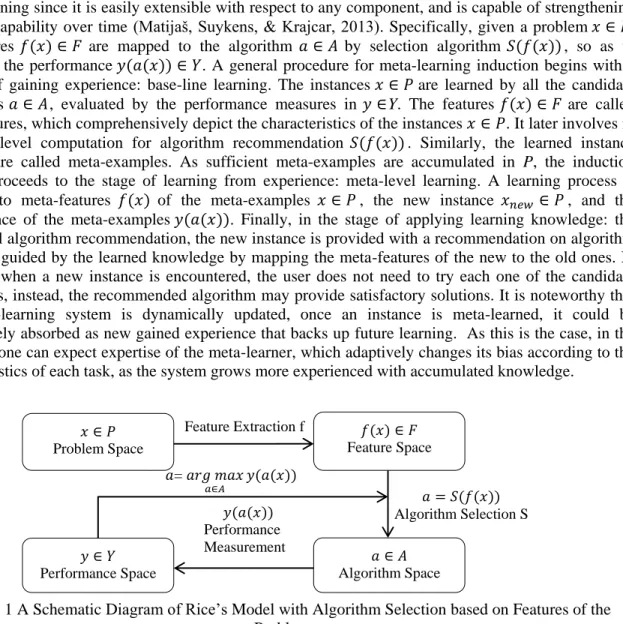
The early contribution related to computer programming on meta-learning dates back to 1986, when STABB (“Shift to A Better Bias”) is proposed by Utgoff (1986), as the first system capable of dynamically adjusting a learner’s bias. Following Utgoff’s work, Rendell, Seshu, and Tcheng (1987) propose a variable bias management system (VBMS), which selects an algorithm (out of three), based on two meta-features: the number of training instances and the number of features. The StatLog project (Brazdil, Gama, & Henery, 1994) further extends VBMS by introducing a larger number of dataset characteristics, together with a broad class of candidate classification models and algorithms for selection. The first formal abstract model for algorithm recommendation corresponds to Rice’s model (Rice, 1975). As shown in Figure 1, Rice’s model has four component spaces: (1) problem space P represents the datasets of learning instances; (2) feature space F includes the features or characteristics extracted from the datasets in P, as an abstract representation of the instances; (3) algorithm space A contains all the candidate algorithms considered in the context; (4) performance space Y is the performance measurement
8 of an algorithm instance in A on a problem instance in P. This framework is well accepted for component-based learning since it is easily extensible with respect to any component, and is capable of strengthening learning capability over time (Matijaš, Suykens, & Krajcar, 2013). Specifically, given a problem 𝑥 ∈ 𝑃, the features 𝑓(𝑥) ∈ 𝐹 are mapped to the algorithm 𝑎 ∈ 𝐴 by selection algorithm 𝑆(𝑓(𝑥)), so as to maximize the performance 𝑦(𝑎(𝑥)) ∈ 𝑌. A general procedure for meta-learning induction begins with a process of gaining experience: base-line learning. The instances 𝑥 ∈ 𝑃 are learned by all the candidate algorithms 𝑎 ∈ 𝐴, evaluated by the performance measures in 𝑦 ∈Y. The features 𝑓(𝑥) ∈ 𝐹 are called meta-features, which comprehensively depict the characteristics of the instances 𝑥 ∈ 𝑃. It later involves in the meta-level computation for algorithm recommendation 𝑆(𝑓(𝑥)). Similarly, the learned instance datasets are called meta-examples. As sufficient meta-examples are accumulated in P, the induction process proceeds to the stage of learning from experience: meta-level learning. A learning process is imposed to meta-features 𝑓(𝑥) of the meta-examples 𝑥 ∈ 𝑃, the new instance 𝑥𝑛𝑒𝑤 ∈ 𝑃, and the
performance of the meta-examples 𝑦(𝑎(𝑥)). Finally, in the stage of applying learning knowledge: the meta-level algorithm recommendation, the new instance is provided with a recommendation on algorithm selection, guided by the learned knowledge by mapping the meta-features of the new to the old ones. In this way, when a new instance is encountered, the user does not need to try each one of the candidate algorithms, instead, the recommended algorithm may provide satisfactory solutions. It is noteworthy that the meta-learning system is dynamically updated, once an instance is meta-learned, it could be immediately absorbed as new gained experience that backs up future learning. As this is the case, in the long run, one can expect expertise of the meta-learner, which adaptively changes its bias according to the characteristics of each task, as the system grows more experienced with accumulated knowledge.
Figure 1 A Schematic Diagram of Rice’s Model with Algorithm Selection based on Features of the Problem.
Based on the Rice’s model, the machine learning community has studied the application of meta-learning for classification problems where the classification algorithm which best labels each data instance to the classes is recommended. As we stated in Section 1, the meta-model for simulation is used to predict continuous outputs, thus regression algorithms shall be studied. A brief review on recommendation for regression problems is given in the next section.
2.2.2
Meta-learning for Regression Problems
The METAL project funded in 1998 by ESPRIT (a meta-learning assistant for providing user support in machine learning and data mining) is among the first few attempts to explore the application of meta-learning for regression problems. The project delivered the Data Mining Advisor (DMA), a web-based meta-learning system for the automatic selection of learning algorithms. In addition, Köpf, Taylor, and Keller (2000) tested the suitability of meta-learning applied to regression problems using primarily the StatLog features. The number of test regression problems is over 5,000, with various sample sizes in the range of (110, 2,000), and 3 candidate regression models were considered. In 2002, Kuba, Brazdil, Soares, and Woznica investigated new features for regression problems, e.g., presence of outliers in the target,
Feature Extraction f 𝑦(𝑎(𝑥)) Performance Measurement 𝑎 = 𝑆(𝑓(𝑥)) Algorithm Selection S 𝑎= 𝑎𝑟𝑔 𝑚𝑎𝑥 𝑎∈𝐴 𝑦(𝑎(𝑥)) 𝑦 ∈ 𝑌 Performance Space 𝑥 ∈ 𝑃 Problem Space 𝑎 ∈ 𝐴 Algorithm Space 𝑓(𝑥) ∈ 𝐹 Feature Space
9 coefficient of variation, etc., providing a supplement to StatLog measures as tested by Köpf et al. (2000). Smith-Miles (2008) pointed out the potential of extending the algorithm selection problem to cross-disciplinary developments, and a unified framework was proposed to generalize the meta-learning concepts for tasks such as regression, sorting, forecasting, constraint satisfaction, and optimization. Smith, Mitchell, Giraud-Carrier, & Martinez (2014) applied a collaborative filtering technique, meta-CF (MCF), for the meta-learning and hyperparameter selection. MCF does not rely on meta-features but only considers the similarity of the performance of the learning algorithms associated with their hyperparameter settings. MCF was validated on 125 data sets and 9 diverse learning algorithms, and shown to be a viable technique for recommending learning algorithms and hyperparameters. M. Smith & White (2014) proposed the machine learning results repository (MLRR), an easily accessible and extensible database for metalearning. MLRR was designed as a data repository to facilitate meta-learning and provide benchmark meta-data sets of previous experiment results, which is a downloadable resource for other researchers.
As we discussed in Section 2.1, traditional meta-modeling approaches fail to provide an effective and efficient way for model selection, resulting in sub-optimal modeling solution and waste of computations. While more investigations have focused on meta-learning on cross-disciplinary studies, the applicability of meta-learning on meta-model selection has yet to be fully defined and studied. In this study, we propose a generalized framework of meta-learning for recommending meta-models specifically designed for data-driven simulation modeling to investigate the suitability of the approach and improvement it could achieve.
3
Proposed Framework
3.1
Recommendation System for Meta-modeling- A Generalized Framework
The proposed framework is built upon Rice’s work (Figure 1) with two main advancements: First, feature reduction component is added to the framework. Second, we expand the meta-learning algorithm into a ranking based method including model-based learners and instance-based learners, to strengthen the recommending capability of the system. The pseudo code of the proposed framework is presented in Figure 2.
Figure 2 A Pseudo Code of Meta-learning Based Recommendation System for Meta-modeling.
3.2
Meta-features
Begin: Given new instance 𝑥𝑛𝑒𝑤∈ 𝑃, meta-examples 𝑥 ∈ 𝑃, feature reduction d, meta-learner algorithm R, accuracy performance measurement 𝑦 ∈ 𝑌
Step 1: Conduct feature extraction 𝑓(𝑥𝑛𝑒𝑤) Step 2: Conduct feature reduction 𝑑(𝑓(𝑥𝑛𝑒𝑤))
Step 3: Meta-learning: find rankings {𝑎1, 𝑎2, … , 𝑎𝑘}, where 𝑎 ∈A, k is the number of algorithm candidates, such that 𝑦(𝑎𝑘−1(𝑥𝑛𝑒𝑤)) ≥ 𝑦(𝑎𝑘(𝑥𝑛𝑒𝑤)) Case meta-learner R OF Model-based algorithm: 𝑎 = 𝑅(𝑑(𝑓(𝑥)), 𝑑(𝑓(𝑥𝑛𝑒𝑤)), 𝑦(𝑥)) Instance-based algorithm: 𝑎 = 𝑅(𝑑(𝑓(𝑥)), 𝑑(𝑓(𝑥𝑛𝑒𝑤))) End Case
10 Before meta-learning is applied, one task to fulfill is to identify available “features of instances that can be calculated and that correlate with hardness/complexity” (Smith-Miles, 2008). The idea behind this is to use learning algorithms to extract a unified body of knowledge from the dataset, which adequately represents the entire dataset for meta-level induction learning. Because the meta-learning algorithm (meta-learner) is sensitive to the underlying structure of the data, the determination and selection of appropriate features is a crucial step.
In this research, the statistical and geometrical meta-features are derived. A total of 15 meta-features are proposed, of which the definitions and calculations are given below. Some of the features are extensively used in meta-learning on classification (Romero, Olmo, & Ventura, 2013; Sun & Pfahringer, 2013). For example, the basic statistical characterizations of the dataset, such as mean, median, standard deviation, skewness and kurtosis. Moreover, geometrical measurements for data characterization, such as the gradient-based features on response values (1-4), outlier ratio (12), ratio of local extrema (13 & 14) and biggest difference (15) are derived. For a thorough review on meta-features specifically for regression problem characterization, we refer the reader to (Köpf et al., 2000; Pavel Brazdil et al., 1994).
Given N sample data points, for the ith sample point, let 𝐺𝑖 be the gradient and 𝑓𝑖 be the response of the
point, point j is the nearest neighbor of point i in Euclidian space. 𝐺𝑖 is calculated as:
𝐺𝑖 = 𝑓𝑖− 𝑓𝑗, i≠ 𝑗. (11)
1) Mean of Gradient of Response Surface Point: Mean of absolute values of gradient, 𝐺̅, which evaluates how steep and rugged the surface is, by looking into its rate of change on the sample data,
𝐺̅ = 1 𝑁⁄ ∑𝑁𝑖=1|𝐺𝑖|. (12)
2) Median of Gradient of Response Surface Point: Median of absolute values of gradient.
3) SD of Gradient of Response Surface Point: Standard deviation of gradient, SD (G) , which evaluates the variation of the rate of change on the sample data,
SD (G) =√1 (𝑁 − 1)⁄ ∑𝑁𝑖=1(𝐺𝑖− 𝐺̅)2 . (13)
4) Max of Gradient of Response Surface Point: Maximum of absolute values of gradients on all response surface points, 𝐺𝑚𝑎𝑥, which gives an upper bound of rate of change on the sample data, a measure of
the degree of sudden change on the surface.
𝐺𝑚𝑎𝑥 = max |𝐺𝑖|, 𝑖 = 1, … , 𝑁. (14)
5) Mean of Function values: Mean of response values, 𝑓̅, which evaluates the general magnitude of the surface
𝑓̅ = 1 𝑁⁄ ∑𝑁 𝑓𝑖
𝑖=1 . (15)
6) SD of Function values: Standard deviation of response values, 𝑆𝐷 (𝑓), which evaluates how bumpy the surface is by looking into each value’s deviation from the mean.
𝑆𝐷 (𝑓) = √1 (𝑁 − 1)⁄ ∑𝑁 (𝑓𝑖− 𝑓̅)2
11 7) Skewness of Function values: Skewness of response values, 𝛾1(𝑓), which evaluates the lack of
symmetry on the surface
𝛾1(𝑓) = 𝐸{[(𝑓𝑖− 𝑓̅) 𝑆𝑡𝑑. (𝑓⁄ 𝑖)]3}, 𝑖 = 1, … , 𝑁. (17)
8) Kurtosis of Function values: Kurtosis of response values, 𝛾2(𝑓), which evaluates the flatness relative
to a normal distribution
𝛾2(𝑓) = 𝐸[(𝑓𝑖− 𝑓̅)4]/(𝐸[(𝑓
𝑖− 𝑓̅)2])2, 𝑖 = 1, … , 𝑁. (18)
9) Q1 of Function values: 25% quartile of response values, which is the lower quartile of function values. 10)Q2 of Function values: 50% quartile of response values, which is the median of function values. 11)Q3 of Function values: 75% quartile of response values, which is the upper quartile of function values. 12)Outlier Ratio: Ratio of outliers of response values, which measures percentage of extreme values
among all. An iterative implementation of the Grubbs Test (Grubbs, 1950), which is a statistical test used to detect outliers is applied in this study.
13)& 14) Ratio of local extrema: Ratio of local minima and maxima within a given neighborhood, which measures the percentage of local fluctuations. Note these measurements can differentiate problems with a bumpy response surface and with a flat response surface. The neighborhood is defined within 5 nearest neighbors in this study.
15)Biggest difference: Averaged local biggest difference of function values, 𝐷̅̅̅̅𝑝, which evaluates the average bumpiness by looking into the difference between “valley” and “peak” on each local area
𝐷𝑝
̅̅̅̅ = 1 𝑠⁄ ∑𝑠𝑝=1𝐷𝑝, 𝑝 = 1, … , 𝑠, (19)
where s is the number of local areas, and 𝐷𝑝 is the difference between “valley” and “peak” on area p.
This measurement gives an estimate on the magnitude of the bumpiness for each response surface. 100 local areas are defined in this study, by dividing the whole design surface into smaller sub areas.
3.3
Meta-learners
Meta-learning algorithms are generally categorized into two groups: instance-based learning and model-based learning (Matijaš, 2013). The former learning method assumes the meta-modeling techniques exhibit similar performance on similar problems, where the similarity is measured by some distance metric, e.g., Euclidean distance. While for the latter, one assumes that an underlying model governs the way that algorithms perform on different problems.
3.3.1
Instance-based Meta-learner
The k-Nearest Neighbor ranking approach is commonly selected as an instance-based learner, due to its efficient and effective performance in numerous applications. One naive approach is to solely learn from the nearest neighbor of the target problem, by calculating the Euclidean distance between the target problem i and the meta-examples:
12 where 𝑥𝑖 is the meta-feature vector of i, and m is the number of meta-examples. The nearest neighbor is found by comparing all the distance measures and target the minimum. We call it the 1-NN method. The k-NN method involves the nearest neighbors search step and a ranking generation step. We first select the k nearest neighbors by calculating the similarity between the test problem and the meta-examples, based on the meta-features. Next, the performance is calculated to make the recommendation. The cosine similarity is calculated as follows:
𝑠𝑖𝑚(𝑖, 𝑗) = 𝑐𝑜𝑠(𝑥𝑖, 𝑥𝑗) = 𝑥𝑖∙𝑥𝑗 √‖𝑥𝑖‖2×√‖𝑥𝑗‖2
, j=1,…, m (21)
The ranking of the algorithm a on the target problem i is predicted as
𝑟𝑖,𝑎=∑𝑗∈𝑁(𝑖)𝑠𝑖𝑚(𝑖,𝑗)𝑟𝑗,𝑎
∑𝑗∈𝑁(𝑖)𝑠𝑖𝑚(𝑖,𝑗) (22)
where 𝑁(𝑖) represents the set of k-NN of problem i.
3.3.2
Model-based Meta-learner
The rank position values of each algorithm are the target (response) in the meta-learning models. A regression-based learner assumes an underlying model between the meta-features and the algorithm rankings, which could be trained by the meta-example datasets. In addition, due to the correlations among the various meta-features, a nonlinear model might be more appropriate. In this study, we choose ANN as it is superior on non-linear function modeling (Fonseca, Navaresse, & Moynihan, 2003) and more robust to noisy and redundant features (Goodarzi, Deshpande, Murugesan, Katti, & Prabhakar, 2009).
3.4
Performance Space
The accuracy metrics reflect the degree of closeness of the meta-model measurement outputs 𝑦̂ to true output y. One global measurement for meta-modeling accuracy used in the performance space Y (see Figure 1) is Normalized Root Mean Square Error (NRMSE)
𝑁𝑅𝑀𝑆𝐸 = √∑𝑁𝑖=1(𝑦𝑖−𝑦̂𝑖)2
𝑁 /(𝑦𝑚𝑎𝑥− 𝑦𝑚𝑖𝑛) (23)
Since the focus of this research is to make a recommendation on the meta-modeling algorithms from the algorithm space, we choose to make the recommendation based on the ranks derived from the NRMSE measures. Ranking is a relative measure which is scale-free and case-wise independent. Since different problems are of different levels of difficulty to be modeled, this may result in varied magnitudes of NRMSE measurements. The use of a relative measure, in this study, rank, shall better facilitate the recommendation process. Given the predicted rankings, two evaluation metrics are introduced:
The Spearman’s rank correlation coefficient (Neave & Worthington, 1989) which is employed to measure the agreement between recommended rankings and ideal rankings. For two samples of size N, the coefficient of the recommended ranks 𝑥𝑖 and the ideal ranks 𝑦𝑖 is computed as
𝜌 = 1 − 6· ∑𝑁𝑖=1𝑑𝑖2
𝑁(𝑁2−1), (24)
where 𝑑𝑖 = 𝑥𝑖− 𝑦𝑖, is the difference of ranks of two samples. The value of 1 represents perfect
agreement while −1, perfect disagreement. A correlation of 0 means that the rankings are not related, which would be the expected score of the random ranking method.
13 Hit ratio: the percentage of exact matches between ideal best performer and recommended best performer among all problems. This is to evaluate the “precision” of the meta-learning algorithms. As a matter of fact, in the case of the meta-model recommendation, users are more concerned if the recommended best performer (top 1) matches the ideal one, so only one meta-model is built and computational efficiency is ensured. Therefore, besides the Spearman’s rank correlation coefficient, the hit ratio is also proposed to comprehensively compare the performance of different meta-learners.
4
Experiments and Results Analysis
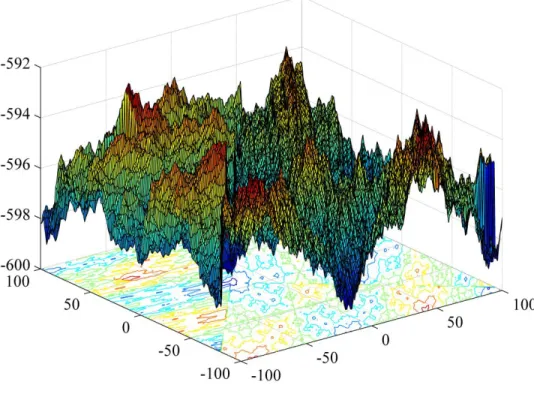
To test the performance of our proposed framework, 44 benchmark functions are collected from IEEE CEC 2013&2014. There are 8 uni-modal functions which have only one global optimum (valley/peak), 28 multi-modal functions which have many local optima (valleys/peaks), and 8 composition functions which are composed of uni-modal and multi-modal functions. For illustration purpose, three 3-dimensional plots for 2-3-dimensional example test functions are given in Figure 3-5 (x, y-axis are the independent (input) variables, and z-axis is the dependent (output) variable).
14 Figure 4 Multi-modal Function: Rotated Weierstrass Function.
15 Note in this study, 10 dimensional functions are studied. These functions are treated as simulation models without prior knowledge for analysis. To simulate stochastic behavior of real world systems, we purposely add uncertainties to the inputs and the outputs of the functions. Specifically, parametric uncertainty (variability on each input variable) and residual uncertainty (variability on the outputs) are considered. Random numbers generated within 10% of each input variable range in [-100, 100] depicts parametric uncertainty. For the residual uncertainty, a random number is added to the training data output, which is generated from a Normal distribution~𝑁(0, 𝜎2), where 𝜎2 equals to 10% times the logarithm of the difference between the maximum and minimum of the training output for each black-box function. Since it is expected that with the existence of uncertainties, the same input does not generate the same output, 25 simulation replicates are conducted. An average value of the 25 output replicates (𝑦̅) is taken as the output for training data while the input for training data takes its nominal value (𝑥), which is the value without noise contamination. And the same operation is applied to the test data.
Three successive experiments are conducted. In the first experiment on meta-modeling, different sizes of training data generated from the benchmark functions are tested on the six meta-models. Meta-models’ performances are sensitive to the number of training data, which will impact the accuracy of model recommendation on meta-learning. Thus we need to decide the appropriate sample size for promising and stabilized meta-modeling accuracy performance. Once the sample size is settled, we implement experiments involving two types of meta-learner models, artificial neural network and k-NN in the second experiments to explore the performance of the meta-learners. In the third experiment, feature (meta-feature) reduction techniques are studied.
4.1
Experiment I – Identification of Meta-modeling Training Size
The objective of this experiment is to identify the appropriate size of the training data to be collected from the simulation. In this experiment, Latin hypercube sampling (LHS) is chosen as the sampling technique on each function of which the design space is set within the range of [-100,100]. LHS is a statistical sampling method used in construction of computer experiments for its good uniformity and coverage from a multidimensional distribution (Eglajs, & Audze, 1977). It is widely used because the sample size is not strictly determined by the number of dimensions of the simulation design space (Zhang, Zhu, Chen, & Arendt, 2012). Moreover, given the sample size is small, it is shown that LHS makes simulations converge faster than traditional random sampling strategies, e.g., Monte Carlo sampling (Matala, 2008).
The six meta-modeling techniques are separately trained on 10-dimensional training datasets of five different training sizes, 80, 100, 150, 300 and 400. In order to avoid over fitting, we implement 5-fold cross-validation on the training process (Kohavi, 1995). 1,000 data points is randomly generated over the design space, which is treated as the testing data set. The grid search method (Chang & Lin, 2011) is implemented on the six meta-models to select the optimal parameters that give the minimum validation error. The test data is applied to the optimally trained model to obtain its generalization error. A multiple comparison test is conducted on the mean estimation of NRMSE of the six meta-models, across the five experiments. As is shown in Figure 6, we observe that the slope of performance improvement is steep from training size 80 to 200, while it changes slowly after 200. Thus the “elbow” point of training size is identified at 300. In the following experiment, all the meta-models are trained with a sample size equal to 300.
16 Figure 6 Multiple Comparison Test on Mean NRMSE of Six Meta-models of Different Sample Sizes.
4.2
Experiment II- Meta-learning for Meta-modeling
The objective of this experiment is to compare the instance-based meta-learner vs. the model-based meta-learner. In this set of experiments, we adopt a leave-one-out strategy, that is, of the 44 problems, 43 are used as a training set, and the remaining one is used to test the resulting meta-learner, which is repeated 44 times (Prudencio & Ludermir, 2004). The average recommendation performance measured by Spearman’s rank correlation coefficients and hit ratio are reported. For each meta-learner, the Spearman’s correlation coefficient is first calculated on each test problem by comparing the learned ranking and ideal ranking of the six meta-models. When all the coefficients are gathered, they are averaged over 44 problems. The hit ratio is calculated as the ratio of the total number of matches on the recommended best performers among the 44 problems.
In this experiment, k-NN is chosen as the instance-based meta-learner, equations (20-21) are applied to identify the exemplar problem for the new studied problem which is then used to identify the appropriate algorithm. ANN is chosen as the model-based meta-learner which takes the following parameter settings: the hidden layer size is tuned within the range of [10, 20], and the transfer functions are selected between radial basis and log sigmoid. We apply 10-fold cross validation with 70% split to training and 30% to validation for prevention of over-fitting. Six ANN models are built on six sets of the rankings of each meta-model across all 44 training problems. Based on the preliminary experiment, we found the k-NN method with k set to 3 is suitable. Table 1 summarizes the overall results of the meta-learners’ recommendation performance on the 44 test problems. In Table 2, the top recommended meta-model given by the meta-learners for each test problem is summarized (the highlighted model is marked as inconsistent with the true best model).
Table 1 Performance Statistics of Meta-learners Meta-learner Spearman’s Correlation Coefficient Hit Ratio
ANN 0.8831 86.36% (38/44)
1-NN 0.5486 81.82% (36/44)
17 As can be seen in Table 1, ANN (model-based meta-learner) outperforms k-NN (1-NN and 3-NN, the instance-based meta-learner) on both Spearman’s correlation coefficient and Hit ratio. Though all three meta-learners are able to recommend the appropriate algorithm for each problem (38, 36, 37 out of 44 test functions), ANN is better at identifying the rankings overall (measured by the Spearman’s correlation coefficient). We believe that this may be due to the fact that the instance-based meta-learner solely relies on the features that characterize the problems. If the features do not adequately represent the picture of the data, it is difficult to find the true similarity between the problems, thus making the learners ineffective on recommending good models. While the model-based meta-learner is a supervised learning approach as it derives the model to relate the meta-features to the meta-model performance. As a result, it may be more tolerant to the noises from the meta-features. In addition, we observe that the performance of 1-NN is lower than 3-NN which indicates that as the number of neighbors increase, the accuracy of k-NN learning improves. Therefore, we conclude that model-based meta-learner generally outperforms instance-based meta-learner.
Table 2 Top Recommended Meta-model Given by Different Meta-learners (K-Kriging, S-SVR, R-RBF, M-MARS, A-ANN, P-PR) Problem # 1 2 3 4 5 6 7 8 9 10 11 12 13 14 15 16 17 18 19 20 21 22 True Best P P R K K K R S K P K K A K K S P P M S S K ANN P P R K K K R S K P K A A K K S P P K S S K 1-NN P R K K K K R S K P K K A K K S P P K R S K 3-NN P P K K K K K S K P K K A K K S P P K R S K Problem # 23 24 25 26 27 28 29 30 31 32 33 34 35 36 37 38 39 40 41 42 43 44 True Best K K R K R R P P P A S K P P P K K K P P K S ANN K K K M K M P P P A S K P P P K K K P P K S 1-NN K K K M K K P P P A S K P P P K K K P P K S 3-NN K K K K K K P P P A S K P P P K K K P P K S
Table 3 summarizes the (approximate) computational cost of the two approaches on each test problem on an Intel i5 CPU 16G computer. Here ANN, the meta-learner example, takes slightly longer time to develop the model compared to the instance-based meta-learner. As seen, the computational efficiency of meta-modeling could be significantly improved from an order of an hour to a minute, by summing up the computational time of 44 functions.
Table 3 (Approximate) Computational Cost Comparison between the Traditional Trial-and-Error Approach and Meta-learning Approach on each test problem
Traditional Trial-and-Error Approach Meta-learning Approach Learning Tasks Meta-modeling with Kriging, SVR,
RBF, MARS,ANN and PR
Feature Extraction,
Meta-learning (ANN) and one meta-modeling with recommended algorithm
Learning Cost 5~10 min. 0.05 sec. + 3~5 sec. + 1~1.5 min.
4.3 Experiment III- Feature Reduction Techniques Comparison
The objective of this experiment is to explore the potential improvements that could be made by employing a feature reduction technique on the meta-learning process. The features defined in Section 3.2 are tentatively selected in the hope that they could effectively represent the dataset. However, it is not guaranteed that all of them are useful. As it is well accepted that redundant and irrelevant features deteriorate the model performance, we propose to use advanced feature reduction techniques to address the noise the curse of dimensionality issues. Three commonly used feature reduction techniques are studied including singular value decomposition (SVD), stepwise regression and ReliefF.
18 SVD is of interest in this research due to its known performance in tolerating data noise (Simek, 2003;
Simek et al., 2004; Phillips, Watson, Wynne, & Blinn, 2009; Chakroborty & Saha, 2010). It is a factorization of a real matrix 𝑋 ∈ 𝑅𝑚×𝑛, 𝑚 ≥ 𝑛,
𝑋 = 𝑈𝑆𝑉𝑡, (25)
where 𝑈 ∈ 𝑅𝑚×𝑚 and 𝑉 ∈ 𝑅𝑛×𝑛 are orthogonal matrices and 𝑆 ∈ 𝑅𝑚×𝑛 is a diagonal matrix. A rank-k (𝑘 ≪ 𝑚𝑖𝑛 (𝑚, 𝑛)) matrix 𝐶 is defined as the best low-rank approximation of matrix 𝑋 if it minimizes the Frobenius norm of the matrix (𝑋 − 𝐶), which is known as the Eckart–Young theorem (Eckart & Young, 1936). This approximation matrix can be computed by SVD factorization and keeping the first k columns of 𝑈, truncating 𝑆 to the first k diagonal components, and keeping the first k rows of 𝑉𝑡. This results in noise reduction by assuming the matrix 𝑋 is low rank, which is not generated at random but has an underlying structure. In this research, the optimal rank of the reduced matrix is solved by the random projection method. The optimal rank is identified as 3 resulting in a feature space dimension reduction from 44 by 15 (44 test functions, 15 meta-features) to 44 by 3 (44 test functions, 3 derived SVD “meta-features”).
Stepwise regression carries out an automatic procedure on the choice of predictive variables when building regression models. It’s a wrapper method which uses a predictive model to score feature subsets. The stepwise regression is set up with bidirectional elimination, with p-value threshold equal to 0.1. As a result, 7 meta-features are selected: (1) max of gradient of response surface point, (2) standard deviation of gradient of response surface point, (3) mean of function values, (4) skewness of function values, (5) kurtosis of function values, (6) Q2 of function values, and (7) outlier ratio. The ReliefF algorithm examines the difference between features of nearby instances and iteratively
updates the weight of each feature, where features are selected with higher averaged weight. Due to the sensitivity of ReliefF to the settings of number of nearest neighbors, we tentatively set the k-value as 5, 10, 15, and 20, and the ranks of the features are averaged across different k values. The averaged ranks decide which features will be selected in the final model. As a result, 10 meta-features are selected: (1) mean of gradient of response surface point, (2) max of gradient of response surface point, (3) median of gradient of response surface point, (4) standard deviation of gradient of response surface point, (5) standard deviation of function values, (6) kurtosis of function values, (7) Q1 of function values (8) Q2 of function values, (9) Q3 of function values, and (10) outlier ratio.
Since we conclude the model-based meta-learner (ANN) outperforms the instance-based meta-learner, in this experiment, we choose ANN as the test case to evaluate the efficacy of the feature reduction techniques. The summary statistics of the three methods is given in Table 4. It is observed that both Spearman’s Correlation Coefficient and hit ratio are improved by using feature reduction, where SVD achieves the best performance. Moreover, the number of successful best performer recommendations increases to 40, resulting in a hit ratio of 90.90%, using SVD. The performance of the reduced ANN model using stepwise regression and ReliefF do not observe significant difference, and compared to SVD, they are both slightly inferior. We contend that SVD may perform well when noise exists as stated by (Baker, 2005). The second conclusion we draw from this experiment is, given the 15 meta-features derived, there is redundancy among the features, therefore employing feature reduction techniques has proved to be valuable in improving the recommendation system performance.
Table 4 Summary Statistics of Three Feature Selection Techniques: SVD, Stepwise Regression and ReliefF
19
Singular Value Decomposition 0.9351 90.90% (40/44)
Stepwise Regression 0.9060 88.64% (39/44)
ReliefF 0.8956 88.64% (39/44)
Without Feature Selection 0.8831 86.36% (38/44)
5
Conclusion
In this paper, we develop a meta-learning framework of a meta-model recommendation system for computation-intensive simulation problems. It addresses the problem of meta-model selection, where appropriate meta-models are recommended for surrogate modeling in substitute for physical models. The learned relationships could be used to make predictions on model rankings for unseen problems. Specifically, we propose a number of novel meta-features such as the gradient-based features for characterizing the geometrical properties of the response surface. Next, we explore the use of different meta-leaners (instance-based vs. model-based). The Model-based learner outperforms the instance-based learner which may be due to the fact that the model-based learner is a supervised method which takes both of the meta-features and the model performance into consideration in the learning process. We further explore the contribution of feature reduction techniques and conclude SVD may significantly reduce the dimensionality of the feature space while retaining the core information, which not only expedites the meta-learning process, but also improves the overall performance.
To demonstrate the applicability and efficacy of the proposed recommendation system, 44 benchmark problems have been tested, including uni-modal, multi-modal and composition problems covering a wide range of feature domains. To evaluate the predictive capability of the proposed framework, we have also implemented various popular meta-modeling methods in the literature, including Kriging, SVR, RBF, MARS, ANN and PR. Computational experiments clearly show that the proposed system significantly improves the computational efficiency on meta-modeling and is consistently capable of recommending appropriate models across the 44 benchmark test cases. The results indicate our proposed framework is able to serve as an alternative approach for traditional meta-modeling tasks, especially when the number of candidate meta-models is large and little prior knowledge of the problems is available.
Regarding to practical advantages and research contribution in expert and intelligent systems, the proposed recommendation system in this work can be used to facilitate the development of various expert systems, such as decision making and support systems. The proposed meta-learning based recommendation system augments the traditional trial-and-error meta-modeling method to a structured and automated form suitable for computer manipulation, opening up many possibilities for using it. The generic system is able to automate and optimize the modeling process without human involvement and excessive computations. It emulates the human’s decision-making ability, which is to reason about knowledge based on past experience to solve complex problems. Specifically, it consists of two components: the knowledge base, which represents facts and rules, and the inference engine, which applies the rules to the known facts to deduce new facts. This work provides practical guidelines in the design, development, implementation, and testing of a meta-model recommendation expert system for simulation engineering and machine learning. Due to these theoretical contributions and advantages, the recommendation system can be applied to the simulation industry to reduce the cost and improve modeling and operation efficiency. Moreover, it is advised to facilitate simulation optimization applications where surrogate modeling is of significant implementation in support of effective model construction and computational cost saving.
While promising, we want to note there is room for improvement. For example, extended efforts on feature characterization on the meta-models for knowledge extraction can be explored. In addition, the ranks used for recommendation are derived from a single NRMSE measure. This may be extended to include multi-criteria metrics, e.g., robustness and computational cost. We believe there is room for
20 improvement on extendibility of candidate models and test case sets, as this study uses a subset of the possible meta-models and test problems available in the literature. Inclusion of other meta-models and test cases may extend the expert system knowledge base. We plan to extend our proposed framework reported in this paper with these future research directions.
For future research suggestions in expert and intelligent systems, the proposed model recommendation system can benefit by automatically identifying the appropriate models for a given task. Therefore, the meta-learning could not only be used in a meta-modeling application, but can also be used in optimization with meta-heuristic algorithms, where hundreds of algorithms are available but little insight has been gained regarding which algorithms perform well on which problems. Similarly, the idea could further inspire or enhance a number of research applications, such as classification, forecasting and general regression tasks, where model selection and model recommendation is of urgent need. For example, in the research fields of complex systems such as aircraft design, the task is a sophisticated system engineering one where multiple disciplines are often involved, such as, aerodynamics, multi-objective optimization, and computationally-intensive processes. Due to the computational efficiency and automatic learning capability of meta-learning, it can be applied in both the optimization process for algorithm selection and the computationally-intensive process for meta-model recommendation. This is especially true when the number of design parts are large, and the parts can be described by shared common features.
Acknowledgement
This research was partially supported by funds from the National Science Foundation award (CNS-1239257), from the United States Transportation Command (USTRANSCOM) in concert with the Air Force Institute of Technology (AFIT) under an ongoing Memorandum of Agreement, and National Science Foundation of China (71501132). The U.S. Government is authorized to reproduce and distribute for governmental purposes notwithstanding any copyright annotation of the work by the author(s). The views and conclusions contained herein are those of the authors and should not be interpreted as necessarily representing the official policies or endorsements, either expressed or implied, of USTRANSCOM, AFIT, the Department of Defense, or the U.S. Government.
References
Acar, E. (2015). Effect of error metrics on optimum weight factor selection for ensemble of metamodels. Expert Systems with Applications, 42(5), 2703–2709.
Baker, K. (2005). Singular value decomposition tutorial. The Ohio State University, 2005, 24.
Banks, J., Carson, J., Nelson, B. L., & Nicol, D. (2004). Discrete-Event System Simulation. PrenticeHall international series in industrial and systems engineering.
Barker, P. A., Street-Perrott, F. A., Leng, M. J., Greenwood, P. B., Swain, D. L., Perrott, R. A., … Ficken, K. J. (2001). A 14,000-year oxygen isotope record from diatom silica in two alpine lakes on Mt. Kenya. Science (New York, N.Y.), 292, 2307–2310.
Barton, R. R. (1992). Metamodels for simulation input-output relations. In Winter Simulation Conference (Vol. 9, pp. 289–299).
21 Bashiri, M., & Farshbaf Geranmayeh, A. (2011). Tuning the parameters of an artificial neural network
using central composite design and genetic algorithm. Scientia Iranica, 18, 1600–1608. Brazdil, P., Carrier, C., Soares, C., & Vilalta, R. (2008). Metalearning: applications to data mining.
Springer Science & Business Media.
Brazdil, P., Gama, J., & Henery, B. (1994). Characterizing the applicability of classification algorithms using meta-level learning. In F. Bergadano & L. De Raedt (Eds.), Machine Learning: ECML-94 SE - 6 (Vol. 784, pp. 83–102). Springer Berlin Heidelberg.
Brazdil, P., Soares, C., & Costa, J. Da. (2003). Ranking learning algorithms: Using IBL and meta-learning on accuracy and time results. Machine Learning, 251–277.
Chakroborty, S., & Saha, G. (2010). Feature selection using singular value decomposition and QR factorization with column pivoting for text-independent speaker identification. Speech Communication, 52(9), 693–709.
Chang, C.-C., & Lin, C.-J. (2011). LIBSVM: A Library for Support Vector Machines. ACM Transactions on Intelligent Systems and Technology, 2, 27:1–27:27.
Clarke, S. M., Griebsch, J. H., & Simpson, T. W. (2005). Analysis of support vector regression for approximation of complex engineering analyses. Journal of Mechanical Design, Transactions of the ASME, 127, 1077–1087.
Cui, C., Wu, T., Hu, M., Weir, J. D., & Chu, X. (2014). Accuracy vs. robustness: bi-criteria optimizaed ensemble of metamodels. Proceedings of the 2014 Winter Simulation Conference, 616–627. De Souto, M. C. P., Prudencio, R. B. C., Soares, R. G. F., de Araujo, D. S. a., Costa, I. G., Ludermir, T.
B., & Schliep, A. (2008). Ranking and selecting clustering algorithms using a meta-learning
approach. 2008 IEEE International Joint Conference on Neural Networks (IEEE World Congress on Computational Intelligence), 3729–3735.
Draper, N., & Smith, H. (1981). Applied regression analysis 2nd ed. Technometrics, 47, 380–380. Drucker, H., & Chris, B. (1997). Support vector regression machines. Advances in Neural Information
Processing Systems 9, 9(x), 155–161.
Drucker, H., Chris, Kaufman, B. L., Smola, A., & Vapnik, V. (1997). Support vector regression machines. In Advances in Neural Information Processing Systems 9 (Vol. 9, pp. 155–161).
Dyn, N., Levin, D., & Rippa, S. (1986). Numerical Procedures for Surface Fitting of Scattered Data by Radial Functions. SIAM Journal on Scientific and Statistical Computing.
Eckart, C., & Young, G. (1936). The approximation of one matrix by another of lower rank. Psychometrika, 1, 211–218.
Efroymson, M. A. (1960). Multiple regression analysis. Mathematical Methods for Digital Computers, 1, 191–203.