Identification and Small-Signal Analysis of Interaction Modes in VSC MTDC Systems

J. Beerten, S. D’Arco, and J.A. Suul, “Identification and Small-Signal Analysis of Interaction

Modes in VSC MTDC Systems,”

IEEE Transactions on Power Delivery

, vol. 31, no. 2, pp.

888-897, Apr. 2016.

Digital Object Identifier:

10.1109/TPWRD.2015.2467965

URL:

http://ieeexplore.ieee.org/xpl/articleDetails.jsp?arnumber=7194813

© 2016 IEEE. Personal use of this material is permitted. Permission from IEEE must be obtained

for all other users, including reprinting/ republishing this material for advertising or promotional

purposes, creating new collective works for resale or redistribution to servers or lists, or reuse of

any copyrighted components of this work in other works.

Identification and Small-Signal Analysis of

Interaction Modes in VSC MTDC Systems

Jef Beerten,

Member, IEEE,

Salvatore D’Arco, Jon Are Suul,

Member, IEEE

Abstract—In this paper, a methodology is presented to identify and analyse interaction modes between converters in Voltage Source Converter Multi-Terminal High Voltage Direct Current (VSC MTDC) systems. The absence of a substantial level of energy stored in such power electronics based systems results in fast system dynamics, governed by electromagnetic phenomena. Moreover, interactions between converters are largely influenced by the control parameters and in general, an a-priori identific-ation of interaction modes based on associated time constants is less straight-forward than in AC systems. Furthermore, the extent to which converters interact not only depends on the controller parameters, but is also influenced by the physical characteristics of the HVDC system. The methodology introduced in this paper is based on aggregated participation factors to distinguish between local modes, primarily associated with one terminal, and interaction modes involving multiple terminals. To illustrate the proposed methodology, the influence of droop control parameters, as well as DC breaker inductors, on the system dynamics and the participation of the terminals in system interactions are investigated for a three-terminal MTDC system.

Index Terms—HVDC transmission, Multi-terminal HVDC, Small-signal dynamics, Converter interactions.

I. INTRODUCTION

In recent years, the power industry is showing an increasing interest in High Voltage Direct Current (HVDC) transmission based on Voltage Source Converters (VSC) in a multi-terminal (MTDC) or even meshed grid configuration to connect off-shore wind farms [1]. Although VSC HVDC technology has been in operation in point-to-point links, the operation of several converters in an MTDC system poses a number of technical challenges. Since larger HVDC grids will most likely be multi-vendor systems with potentially different converter technologies operating in the same grid, a critical aspect concerns the interoperability and the prediction of possible adverse interactions between the terminals. In AC systems, the fundamentals of adverse interactions between generat-ors are well understood and small-signal stability analysis is typically distinguishing between local modes and slower

Jef Beerten is funded by a postdoctoral research grant from the Research Foundation – Flanders (FWO). The work of SINTEF Energy Research in this paper was supported by the project “Protection and Fault Handling in Offshore HVDC Grids – ProOfGrids,” financed by the Norwegian Research Council together with industry partners EDF, National Grid, Siemens, Statkraft, Statnett, Statoil and NVE.

Jef Beerten is with the Department of Electrical Engineering (ESAT), Division ELECTA & EnergyVille, University of Leuven (KU Leuven), Kasteelpark Arenberg 10, bus 2445, 3001 Leuven-Heverlee, Belgium (e-mail: [email protected]). Salvatore D’Arco is with SINTEF Energy Re-search, 7465 Trondheim, Norway (e-mail: [email protected]). Jon Are Suul is with the SINTEF Energy Research, and also with the Department of Electric Power Engineering, Norwegian University of Science and Technology (NTNU), 7495 Trondheim, Norway (e-mail: [email protected]).

interarea modes [2]. Furthermore, the synchronous generators’ inertia provides a physical basis for this classification of AC system stability phenomena [3]. This does not directly apply to HVDC grids, where the time constants governing the system response are much smaller as they are determined by the capacitive discharge of the cables and converter DC capacitors. Consequentially, the controller settings can have a significant impact on the nature of the interactions, which are not necessarily limited to the converters, but can also involve other system elements.

Since most operating VSC HVDC schemes until today are two-terminal systems with a centralised DC voltage control, the stability analysis has mainly been limited to the interaction with the AC system. For the analysis of local interactions with the power system, the converter can usually be simplified as a controllable voltage source, whilst retaining a detailed representation of the converter controllers [4], [5]. Moreover, a reduced model of the AC system, namely a voltage source with a complex impedance based on the short-circuit ratio (SCR) at the Point of Common Coupling (PCC), is generally used to study the stability of the controller with respect to the local AC system [6], [7]. For such studies, the DC side can usually be simplified by only retaining the overall voltage dynamics in the system [5], [7]. For studying interactions with slower multimachine dynamics in AC systems, the converter control is commonly simplified, by focussing on the slower power control dynamics [8].

The expected advent of multi-terminal systems has triggered the development of a new breed of linearised models to study control interactions involving several converters [8]–[13]. In [9], the stability of voltage droop controlled converters in a DC system was discussed using singular value decomposition of a linearised model of the converter controllers and the DC system. However, the focus was on the voltage droop gain and possible adverse interactions with other control loops were not included. Furthermore, the DC grid dynamics were accounted for by lumped impedance models. In [10] and [11], MTDC small-signal stability models were developed by straightforwardly extending the operation principles of two-terminal schemes. The models in both works did not account for a distributed voltage control based on a droop control action, which is generally conceived as the most plausible candidate for controlling the DC system voltage in future meshed HVDC grids. In [10], the main focus was on the development of the converter models, whilst the DC system was modelled as a resistive-capacitive network. While this simplified system representation might contain enough details to study the slower AC/DC system interactions, it implies only a partial image of all possible converter interactions. Moreover,

PLL  dc v 1 6 g PWM dq abc abc m Current Control d m abc dq * ld i * lq i ld i ilq Locked Phase Loop , ac f p q m dc C dc v f L l I l i f C T Z o v o I PCC o V PLL  PLL  Power/ Control * ac p Power Measurement , ac f p vo l i Voltage * dc v





Figure 1. Converter control layout.

none of the studies considers the possible adverse influence of the DC breakers’ inductors on the DC voltage control stability, which was recently taken into account in [14].

A first step towards assessing the potential for problems related to adverse small-signal interactions in a MTDC system can be to identify the modes of the system that are not only associated with a single terminal. Moreover, a methodology to identify interaction modes in the system can help to provide a more fundamental understanding of the system dynamics. In this context, it should be emphasised that the presence of interactions in an MTDC system does not necessarily imply negative effects since terminals in an MTDC system are meant to interact in order to transfer power. However, if some of the interaction modes become poorly damped, they can give rise to oscillations that cannot be addressed locally.

This paper aims at introducing a method for systematically identifying interaction modes in a VSC MTDC system by analysing the participation pattern of the different system elements. Thus, the paper demonstrates how the modes can be classified into local and interaction modes, in a way similar to the subdivision generally applied in large AC systems. As an example, the paper addresses the extent to which the converter interactions are influenced when the overall system control is changed from centralised voltage control to voltage droop control and investigates the influence of the DC breakers’ inductors on the interaction modes.

II. MATHEMATICAL MODELLING

To maintain the flexibility to model systems with arbitrary topologies, the different elements in the HVDC scheme (cables and converters) are first represented as independent linearised time-invariant subsystems in a state-space format:

˙

x=Ax+Bu; x(0) =x0, (1) with x∈ Rn the state vector,u ∈Rm the input vector and A ∈ Rn×n, B ∈ Rn×m the known coefficient matrices that can be a function of the steady-state linearisation aroundx0∈ Rn. The dynamics for the entire system are thereafter derived by assembling the subsystem models. Further details on the general modular state-space modelling procedures for multi-converter systems are found in [15], [16].

− + v∗ dc vdc,f Kdc 1 + 1 τdc·s i∗_ld

(a) Constant DC voltage control

− + p∗ ac pac,f KP 1 + 1 τP·s i∗_ld

(b) Constant power control

+ − v∗ dc vdc,f gdc + − + ∆pac p∗ ac pac,f KP 1 + 1 τP·s i∗ld

(c) Voltage droop control Figure 2. Converter outer power/voltage control loops.

vg Rg Lg io Cf vo Rf Lf il vi vdc Cdc idc

Figure 3. Converter terminal representation for state-space modelling.

A. Converter terminal modelling

The converter and its control loops can be derived in the form of (1). The converter model used in this study is largely based on the model described in [17] with a control system configuration as depicted in Fig. 1. It consists of an averaged two-level converter model, including filter bus dynamics. The connection to the grid is taken into account using a complex impedance, which represents the combination of the transformer and the grid Thevenin impedance. A phase-locked loop (PLL) is used to synchronise the dq reference frame to the voltage at the filter bus. Additional control loops include decoupled inner current controllers, a proportional integral (PI) DC voltage controller (Fig. 2a) or a PI active power controller (Fig. 2b) [13], possibly supplemented with a DC voltage droop (Fig. 2c). Outer control loops for the reactive power have been left out of the study.

The state variables of the resulting 18th _{order converter} model are given by

x= [vod voq ild ilq γd γq iod ioq φd φq · · ·

vpll,d vpll,q pll δθpll vdc vdc,f ρor κ pac,f]T,

(2) with vodq, ildq, iodq, vdc representing the filter bus voltage,

converter currents, grid side currents and DC voltage respect-ively. The integrator states of the PI controllers for the currents, active power or DC voltage are given byγdq,ρandκ, whereas

pll represents the integrator state of the PLL PI controller.

Furthermore, φdq, vpll,dq are the states of voltage low-pass

filters used for the implementation of AC active damping and the PLL, whereas vdc,f and pac,f are filtered values of DC

voltage and active power. The stateδθpll represents the phase

angle displacement between the grid voltage source and the

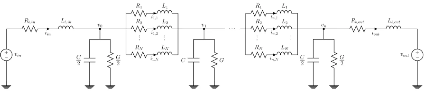
+ − vin Rb,in iin Lb,in v0 C 2 G 2 R1 L1 i1,1 R2 L2 i1,2 .. . ... RN LN i1,N v1 C G · · · R1 L1 in,1 R2 L2 in,2 .. . ... RN LN in,N C 2 G 2 vn Rb,out iout Lb,out + − vout

Figure 5. Equivalent cable model for a frequency-dependent state-space representation.

+ − vin

iin

Rb,in Lb,in Rb,out Lb,out

+ −

vout

iout

Figure 4. Cable terminated by inductors.

The input vectoruconsists of the reference signals shown to the left in Fig. 1 (p∗

ac,vdc∗,i∗lq), as well as the AC grid voltage

amplitudevgand the DC currentidcas indicated in Fig. 3. This

results in a model, in which the converter DC voltage appears as the state variable that needs to be linked with the other subsystems of the MTDC system. The steady-state conditions can be calculated for this building block by assuming a certain operating condition for the entire system and are used to linearise the system model around the operating point.

B. Cable modelling

The HVDC cables are modelled with a state-space repres-entation based on cascaded pi elements with parallel series branches as in [18]. The parallel branches of the pi elements, calculated using vector fitting [19], allow to incorporate the frequency dependence of the series cable parametersRandL. Fig. 4 illustrates how the cable is modelled as an independent building block, terminated with inductors Lb to represent the

current limiting reactors of DC breakers and its corresponding resistance Rb. Fig. 5 shows an equivalent circuit model from

[18], suitable for a state-space representation of the cable. The expressions in the appendix indicate how the state-space model from [18] is extended to account for the presence of the DC breakers.

C. Aggregation of subsystem models

With all different subsystems described in the form of (1), a state-space model of the entire system is assembled.

A first step is to determine the steady state condition for the entire system in order to define the operating point for each subsystem. Hence, a steady-state solution for the DC system is required, taking into account the DC system losses. As a result, one obtains the state-space models of the different subsystems. For subsystem i

˙

xi=Aixi+Biui, (3)

with xi∈Rni _{the subsystem’s state variables, u}

i∈Rmi _the

input variables, Ai∈Rni×ni _{the state-space matrix and B}

i∈

Rni×mi _{the input matrix.}

The overall system matrix At can be assembled by

ac-counting for the “interface variables”, i.e. state variables of subsystems that are input variables for other subsystems. More specifically, these are the DC currents at the cable ends and the converter DC voltages. The state-space model for a system of pelements can be written as

˙ xt=Atxt+Btut, (4) with xt= x1 . . . xp T , (5) ut= _ur 1 . . . u r p T . (6)

assuming no overlapping states in the modelling of the sub-systems, xt∈Rnt _{with n}

t= P p

i=1ni. The resulting input

vector ut∈Rmt _{only consists of reduced versionsu}r

i∈R

mr i of the converter input vectors, since the DC currents, which are inputs to the converter model (Fig. 3), are state variables related to the cable subsystems. Similarly, the DC voltages are state variables related to the converters’ subsystems and the input vector for the cable j is eliminated by substituting the corresponding columns ofBj inAt.

III. IDENTIFICATION OF SUBSYSTEM INTERACTIONS

The interactions between the different subsystems are stud-ied with the model from (4)–(6). As a first step, a criterion is defined to classify the modes as either local or interaction modes, where interaction modes are defined as modes in which at least two converters participate. The interactive nature of these modes can be identified on the basis of participation factors. Letpkidenote the participation factor of state variable

xk in modei, defined as [2]

pki=φkiψik, (7)

withφki thek-th entry of the right eigenvectorφi∈Rnt _and

ψik thek-th entry of the left eigenvectorψi∈Rnt_{. Letp}

i∈

Rnt _{be the vector with the participation factors associated with} modeifor all system states. Similarly,pα,i∈Rnα_{is the vector} for all states of subsystemα.

A parameter ηαi is defined as a measure for the overall

participation for each subsystemαin mode isuch that

ηαi=

kpα,ik

kpik

0 20 40 60 80 100 0 20 40 60 80 100 0 20 40 60 80 100 A B C subsystem a (_ˆη a₎ subsystem b( ˆ ηb) subsystemc(ηˆc)

3 subsystems 2 subsystems local mode

Figure 6. Subsystem interaction representation.

∼

=

1

2

∼

₌

3

∼

₌

P

P

P

Figure 7. Three-terminal VSC MTDC system configuration.

withk · kdenoting theL1-norm. Specifying a thresholdχ, an interaction modeibetween two subsystemsaandbis defined as a mode for which bothηai> χandηbi> χ, resulting in a

subset of interaction modes Sa,b_.

The definition can be extended to more subsystems. When particularly interactions between a subset of subsystemsI are of interest, a set of interaction modes S can be defined as

S={i|ηαi> χ,∀α∈ I}, (9)

Analogously, a subset of interaction modes SA _{is defined,} consisting of modes in which some, but not all subsystems inIare involved. WithIA_{denoting the subset of subsystems} from I

SA=i|ηαi> χ,∀α∈ IA andηβi≤χ,∀β∈ IB ,

(10) with the set of subsystems IB _{defined asI}B_{=I \ I}A_.

The relative participation of subsystems α with respect to the subset I can be defined as

ˆ ηαi= ηαi P x∈I ηxi . (11)

As a generic example, in case where a subset of three sub-systems a,b andcis considered, a so-called ternary diagram can be used to represent the relative participation of each of the three subsystems. Fig. 6 offers an example with an illustrative thresholdχof 10%. The location of the modes in this diagram determines the relative participation of the three subsystems. Mode A is a mode in which the three subsystems participate about equally. The area marked in dark grey contains all the modes in which the three converters participate. Similarly, mode B has about equal participation from subsystemsa, and

b, whilst subsystemcdoes not participate in the mode. Mode C

0.00 0.20 0.40 0.60 0.80 1.00 1.00 1.10 Time t (s) DC V oltage udc (p.u.) 1 2 3 1 - lin 2 - lin 3 - lin (a) 0.00 0.20 0.40 0.60 0.80 1.00 −1.0 −0.5 0.0 0.5 Time t (s) d -current iod (p.u.) 1 2 3 1 - lin 2 - lin 3 - lin (b)

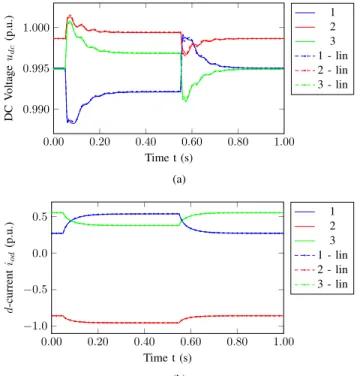
Figure 8. Time-domain comparison – system response to voltage setpoint change. 0.00 0.20 0.40 0.60 0.80 1.00 0.990 0.995 1.000 Time t (s) DC V oltage udc (p.u.) 1 2 3 1 - lin 2 - lin 3 - lin (a) 0.00 0.20 0.40 0.60 0.80 1.00 −1.0 −0.5 0.0 0.5 Time t (s) d -current iod (p.u.) 1 2 3 1 - lin 2 - lin 3 - lin (b)

Figure 9. Time-domain comparison – system response to active power setpoint change.

on the other hand, is a ‘local’ mode associated with subsystem

c, but not with subsystems a and b. Attention needs to be paid to the fact that the position in the ternary diagram only indicates the relative contributions of the three subsystems (ηˆαi). In other words, when there are more than three elements

in the system and when, for a given mode i,ηΣIi <1 with

ηΣIi =

P

x∈Iηxi, the position of the mode in the diagram

−600 −400 −200 0 −10000 −5000 0 5000 10000 Real Imag

(a) EigenvaluesAt (system)

−300 −200 −100 0 −4000 −2000 0 2000 4000 Real Imag (b) Modes converter 1 (η1>5%) −600 −400 −200 0 −10000 −5000 0 5000 10000 Real Imag (c) Cable modes (η1-2+η2-3>50%) −300 −200 −100 0 -2000 -1000 0 1000 2000 A B C D E F G H Real Imag

(d) Converter interaction modes (ηco>5% for at least 2 converters)

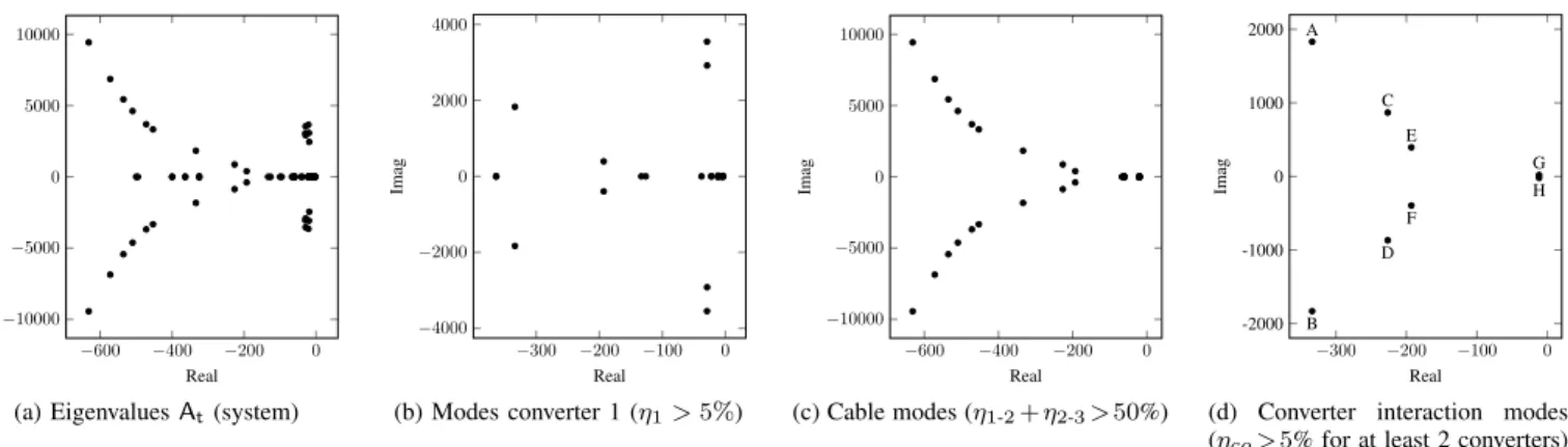
Figure 10. Pole location of the system matrixAt, modes related to converter 1, cable modes, converter interaction modes – power control on converters 1 and 3, voltage control on converter 2.

vod_voq ildilqγd_γq iodioq φd_φq vpll,d_vpll,qpl l δθpl l vdc vdc,f ρor κ pac,f 0 0.2 0.4 0.6 0.8 1 Normalised participation factor conv 3 conv 2 conv 1

(a) Participation in modes C,D

vod_voq ildilqγd _γq iodioq φd _φq vpll,d_vpll,qpl l δθpl l vdc vdc,f ρor κ pac,f 0 0.2 0.4 0.6 0.8 1 Normalised participation factor conv 3 conv 2 conv 1

(b) Participation in modes E,F

vod_voq ild ilq γd _γq iodioq φd_φq vpll,d_vpll,qpl l δθpl l vdc vdc,f ρor κ pac,f 0 0.2 0.4 0.6 0.8 1 Normalised participation factor conv 3 conv 2 conv 1 (c) Participation in modes G,H Figure 11. Participation in selected interaction modes – voltage control in converter 2, power control in converters 1 and 3.

0 20 40 60 80 100 0 20 40 60 80 100 0 20 40 60 80 100 A,B C,D E,F G,H con verter 1 (_ˆη 1₎ con verter 2( ˆ η2) converter3(ηˆ3) 0 0.2 0.4 0.6 0.8 1 con v erter participation P ˆ ηco

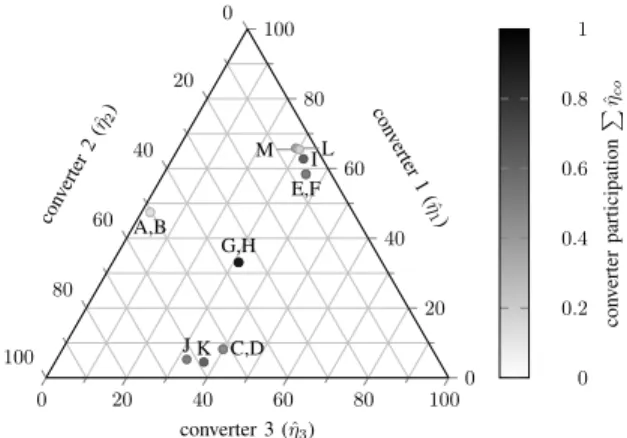
Figure 12. Converter participation in interaction modes – power control on converters 1 and 3, voltage control on converter 2.

the three elements compared to each other. The contribution of the other elements in the network will be visualised in the ternary diagram by grouping these remaining elements and changing the luminance accordingly. Another consequence is that the shaded areas cannot directly be applied for the modesi

for whichP

x∈Iηˆxi<1, as the absolute relationηαi> χturns into a relative one as a result of the scaling, henceηˆαi>χˆwith

ˆ

χ=χ/ηΣIi. Consequentially, the area indicating interactions

between the three subsystems shrinks accordingly with lower

values of ηΣIi.

IV. CONVERTER INTERACTIONS INMTDCSYSTEMS

The identification method from the previous section is applied to a three-terminal MTDC system. The configuration, shown in Fig. 7, is based on a symmetrical monopolar system with voltage ratings of±320kV. The three converters and the cables have a rated power of 1200 MW. The cable between converters 1 and 2 is 300 km long, whereas the cable between converters 2 and 3 is 150 km long. Cable data are based on the model presented in [20]. The AC side parameters of the two-level converter configuration have been taken from [21]. The inner current controller has been tuned to obtain a critically damped system with an equivalent time constant of 2.5 ms.

A. Time-domain model verification

Figs. 8–9 show a time-domain verification of the linearised model (index ‘lin’) against a non-linear three-phase averaged model in MATLAB/Simulink SimPowerSystems, using DC voltage droop control according to Fig. 2c on all converters. The active power PI controller has been tuned to obtain an equivalent time constant of 25 ms (hence 10 times slower than inner current controller), while a droop gain of 10 has been used, resulting in a theoretical second order system response with damping ζ = 0.15 and frequency f0 = 21 Hz. Cable models with 3 parallel branches and 3 pi sections have been

−600 −400 −200 0 −10000 −5000 0 5000 10000 Real Imag

(a) EigenvaluesAt (system)

−300 −200 −100 0 −4000 −2000 0 2000 4000 Real Imag (b) Modes converter 1 (η1>5%) −600 −400 −200 0 −10000 −5000 0 5000 10000 Real Imag (c) Cable modes (η1-2+η2-3>50%) −300 −200 −100 0 -2000 -1000 0 1000 2000 A B C D E F G H I JK L M Real Imag

(d) Converter interaction modes (ηco>5% for at least 2 converters)

Figure 13. Pole location of the system matrixAt, modes related to converter 1, cable modes, converter interaction modes – droop control on all converters.

vod_voq ildilqγd_γq iodioq φd_φq vpll,d_vpll,qpl l δθpl l vdc vdc,f ρ pac,f 0 0.2 0.4 0.6 0.8 1 Normalised participation factor conv 3 conv 2 conv 1

(a) Participation in modes C,D

vod_voq ildilqγd _γq iodioq φd _φq vpll,d_vpll,qpl l δθpl l vdc vdc,f ρ pac,f 0 0.2 0.4 0.6 0.8 1 Normalised participation factor conv 3 conv 2 conv 1

(b) Participation in modes E,F

vod_voq ild ilq γd _γq iodioq φd_φq vpll,d_vpll,qpl l δθpl l vdc vdc,f ρ pac,f 0 0.2 0.4 0.6 0.8 1 Normalised participation factor conv 3 conv 2 conv 1 (c) Participation in modes G,H vod_voq _ildilqγd_γq iodioq φd_φq vpll,d_vpll,qpl l δθpl l vdc vdc,f ρ pac,f 0 0.2 0.4 0.6 0.8 1 Normalised participation factor conv 3 conv 2 conv 1 (d) Participation in mode I vod_voq _ildilqγd _γq iodioq φd _φq vpll,d_vpll,qpl l δθpl l vdc vdc,f ρ pac,f 0 0.2 0.4 0.6 0.8 1 Normalised participation factor conv 3 conv 2 conv 1

(e) Participation in mode J

vod_voq _ild ilq γd _γq iodioq φd_φq vpll,d_vpll,qpl l δθpl l vdc vdc,f ρ pac,f 0 0.2 0.4 0.6 0.8 1 Normalised participation factor conv 3 conv 2 conv 1 (f) Participation in mode K Figure 14. Participation in selected interaction modes – droop control.

used, based on a trade-off between accuracy and simulation speed. Fig. 8 shows the effect of a 10 % step change in voltage references for all converters at t=0.05 s and back to the original values at t=0.55 s, on the DC voltage vdc and

active component of the grid side currentsiod. As expected, the

picture shows that the linearised model accurately represents the system in the vicinity of the steady-state operating point used for the linearisation. Similarly Fig. 9 shows the effect of a simultaneous power setpoint change of respectively 0.3 p.u, -0.1 p.u. and -0.2 p.u. for converters 1, 2 and 3. From these curves, it can be seen that the currents are accurately represented, even with a large step in power reference, whereas there are small deviations in DC voltages when the system is not at the linearisation point. The main deviations stem from the non-linearity of the VSC power balance, but this effect

only has a relevant impact for relatively large excursions from the linearisation point.

B. Centralised voltage control

In a first case study, converter 2 is set to constant voltage control, whilst converters 1 and 3 are in constant power mode. In analogy to the previous section, the time constant of the compensated outer power control loop is 10 times larger than the one of the compensated inner current control. The DC voltage control is tuned by means of a symmetrical optimum (phase margin 65◦), with an overall DC system time constant of 22.3 ms, of which 5.4 ms results from each converter in the system. The inverted power in converters 1 and 3 are set to 150 MW and 500 MW, resulting in a rectified power in converter 2 of 662 MW. The cables have been represented by

the model from [18], with 5 parallel branches and 5 parallel sections.

Fig. 10a shows the eigenvalues of the entire system, limited to the ones with the real part over -1000. As a result, the plot is limited to 86 relevant modes out of a total of 112 modes. Fig. 10b depicts the eigenvalues related to converter 1 (i.e. η1 > 5%). Fig. 10c shows the cable modes (i.e. modes for which the sum of the cable participationη1-2+η2-3is over50%). Fig. 10d shows the interaction modes between converters, i.e. the modes for which ηco >5% for at least two converters. With

this threshold, only a limited subset of 8 out of 112 modes are identified as interaction modes between the converters.

Fig. 11 shows the normalised values of the participation factors for a selection of interaction modes. These values are defined as |pki|/kpik, withk · k the L1-norm. The converter states in the figures are defined in (2). Modes A and B are not depicted, since they are mainly cable modes. It is clear from this picture that the main participating states in interaction modes C,D and E,F are the DC voltages vdc.

The main states participating in the slow modes G,H are the three DC voltages, which participate equally, as well as the state κ, which is related to the integrator of the DC voltage controller in converter 2 and to a lesser extent to the corresponding converter current componentild, associated

with the active power. Fig. 12 shows the relative share of the different converters in the interaction modes A to H. The greyscale indicates the combined participation of all converters in the modes. The lighter the circles, the lower the overall converter participation, and consequentially, the higher the overall cable participation. It is clear that modes A,B are mainly associated with the cables, and that the slow modes G,H are mainly associated with the converters. The latter modes are strongly related to the power flow control. However, the results from Fig. 10d reveals that the converter interactions in the DC system are not limited to these slow control modes. Fig. 11 shows that the coupling is mostly associated with the DC voltage and associated states.

C. Voltage droop control

When using voltage droop control, the interaction pattern changes. The droop gain has been designed as explained in Section IV-A and is set to 10 for all converters. The active power of the converters is now equal to 327 MW, -1019 MW and 676 MW for respectively converters 1, 2 and 3. As in the previous section, Figs. 13–14 show the modes and the participation of the different converter state variables in a subset of interaction modes. The interaction modes A to F, which are associated with the cables remain largely unchanged when droop control is added. The interacting states in the slow control modes G,H now include the state variables ρ

related to the integrator in all active power PI controllers and the corresponding current components ild to a lesser extent.

Furthermore, also other real poles appear in the interaction pattern. Fig. 14 shows the participation of the interacting states for modes I to K as an example, in addition to interaction modes analysed in the previous section. Modes I to K are mostly related to the state variable ρ associated with the integrating control action of power controller.

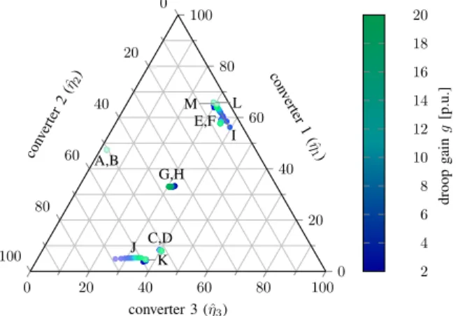
0 20 40 60 80 100 0 20 40 60 80 100 0 20 40 60 80 100 A,B C,D E,F G,H I J K L M con verter 1 (_ˆη 1₎ con verter 2( ˆ η2) converter 3 (ηˆ3) 0 0.2 0.4 0.6 0.8 1 con v erter participation P ˆ ηco

Figure 15. Converter participation in interaction modes – droop control.

−200 −150 −100 −50 0 −1000 0 1000 A B C D E F I J G H K L M Real Imag 100 200 300 400 DC break er inductance Lb [mH]

Figure 16. Interaction modes – variation of DC breaker inductanceLb.

Fig. 15 depicts the relative participation of the different converters in the interaction modes. Comparison with Fig. 12 shows that the participation pattern of the interaction modes associated with the cables (A to F) does not change when the droop control is added. The different operating point does not affect the interaction pattern significantly. As a result of equal droop settings in all converters, the slow interaction mode G,H now faces equal participation from all converters, whereas it was primarily determined by the voltage controlling converter 2 in Fig. 12. The interaction modes J and K are close to the (cable) interaction modes C,D, indicating a similar relative participation of the converters. A similar remark holds for modes I, L and M on the one hand and modes E,F on the other hand. This was also visible from Fig. 14. When the voltage control is distributed by means of voltage droop control, the interactions between the converters are thus no longer limited to the DC voltage states, but also to related converter states. This indicates that poorly damped oscillations or instability caused by the modes G,H should be addressed in a systemwide manner by changing the droop or power controller parameters. Meanwhile, it is clear that in this particular case, there is no need to study modes A-F in more detail due to their high damping.

V. PARAMETRIC SENSITIVITY OF INTERACTION MODES

In this section, the effect of parameter variations to the location and relative participations of the interaction modes

0 20 40 60 80 100 0 20 40 60 80 100 0 20 40 60 80 100 A,B C,D G,H I E,F J K L M con verter 1 (_ˆη 1₎ con verter 2( ˆ η2) converter 3 (ηˆ3) 100 200 300 400 DC break er inductance Lb [mH]

Figure 17. Converter participation in interaction modes – variation of DC breaker inductanceLb. 0 100 200 300 400 0 0.5 1 DC breaker inductanceLb(mH) Cumulated subsystem participation η cable 2-3 cable 1-2 conv 3 conv 2 conv 1

Figure 18. Participation modes E&F – variation of DC breaker inductance

Lb.

are analysed. This illustrates how the proposed classification can be used to study the impact of system parameters on the interaction patterns in the system. The analysis has been limited to voltage droop control on all converters with realistic parameter changes, resulting in a stable system response.

A. Variation of DC breaker inductance

As a first example, inductors are added at the cable ends to represent the effect of DC breakers. Figs. 16–17 respectively illustrate the effect on the position of the poles in the complex plane and of the participation of the converters when changing their values from 10 mH to 400 mH. The colour change (blue to green) illustrates the effect of increasing the DC breaker inductor. In addition, similarly to the greyscale in previous ternary diagrams, the lightness of the colour indicates the over-all cable participation in the mode: the lighter the circles, the lower the overall converter participation, and consequentially, the higher the overall cable participation. It is clear from Fig. 16 that adding the inductors largely leaves the position of (power) interaction modes G,H unaltered, while the modes A to F become much less damped and lower in frequency as a result of the increasing inductance. Contrary to the results in the previous section, increasing the inductance might cause modes A-F to significantly influence the system dynamics.

From Fig. 17, it can be observed that the participation of converter 1 slightly increases for modes G,H, mostly at the

−300 −200 −100 0 −2000 −1000 0 1000 2000 A B C D E F I J G H K L M Real Imag 2 4 6 8 10 12 14 16 18 20 droop g ain g [p.u.]

Figure 19. Interaction modes – variation of droop gaingin all converters.

0 20 40 60 80 100 0 20 40 60 80 100 0 20 40 60 80 100 A,B C,D E,F G,H J I K L M con verter 1 (_ηˆ 1₎ con verter 2( ˆ η2) converter 3 (ηˆ3) 2 4 6 8 10 12 14 16 18 20 droop g ain g [p.u.]

Figure 20. Converter participation in interaction modes – variation of droop gaingin all converters.

expense of converter 3. At the same time, modes C,D and K face a similar, but more pronounced change in participa-tion from the different converters. Whereas these interacparticipa-tions are initially primarily linked with the shorter cable between converters 2 and 3, they now present an increased share of converter 1, the remote converter, since the relative difference between the overall inductance of connections 1-2 and 2-3 decreases. Similarly, modes E,F, which are primarily linked to an interaction between converters 1 and 3, now face an increased share of converter 3 due to the relatively larger increased inductance of connection 2-3. Fig. 18 highlights how the increased share of converter 3 in the mode largely comes at the expense of the participation of cable 1-2.

B. Variation of all droop gains

A variation of the droop gaing from 2 to 20 is considered for all converters. Figs. 19–20 summarise the results. Increas-ing the droop gain slightly changes the position of the cable modes C to F, whilst the relative participation of the converters largely remains unchanged. Mainly modes I and J, which are related to the integrating part of the power controller, face a change in the relative converter participation. The relative converter participation for the slow control modes G,H does not change significantly, but with increasing system gain,

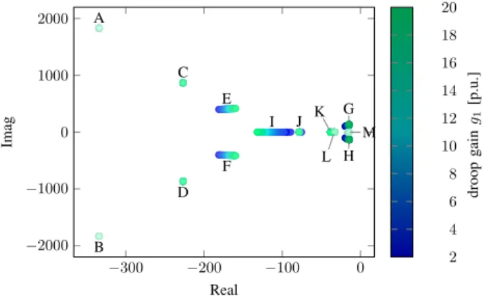
−300 −200 −100 0 −2000 −1000 0 1000 2000 A B C D E F I J G H K L M Real Imag 2 4 6 8 10 12 14 16 18 20 droop g ain g1 [p.u.]

Figure 21. Interaction modes – variation of droop gaingin converter 1.

0 20 40 60 80 100 0 20 40 60 80 100 0 20 40 60 80 100 A,B C,D G,H E,F L J K I M con verter 1 (_ˆη 1₎ con verter 2( ˆ η2) converter 3 (ηˆ3) 2 4 6 8 10 12 14 16 18 20 droop g ain g1 [p.u.]

Figure 22. Converter participation in interaction modes – variation of droop gaingin converter 1.

the corresponding frequency increases whilst the damping decreases.

C. Variation of droop gain in converter 1

As a last example, the droop gain in the remote converter 1 is varied, whilst the gain in converters 2 and 3 is left unchanged at 10. Figs. 21–23 show the results. After comparison with the previous case, it is clear that changing only one droop gain has a greater effect on the relative converter participation in the interaction modes. For example, the relative participation of converter 1 in the slow mode G,H almost doubles. Modes C,D, which initially have a low participation from converter 1 (Fig. 14a), are not affected. Mode I, which had a relatively large share of converter 1 (Fig. 14d), is largely affected, both in position and subsystem participation. The position of mode J remains largely unchanged, whilst the subsystem participation changes for small values of g1 (Fig. 23).

VI. CONCLUSIONS

The classification method presented in this paper allows to accurately distinguish between local converter modes and HVDC system interaction modes. Hereby, the method offers an extension of the widely adopted concept of local and interarea modes in AC systems to MTDC systems. Moreover,

5 10 15 20

0

0.5

1

droop gaing1(p.u.)

Cumulated subsystem participation η cable 2-3 cable 1-2 conv 3 conv 2 conv 1

Figure 23. Participation mode J – variation of droop gaing1 in converter 1.

this approach can assist in identifying possible sources of inter-actions between terminals and in designing corrective inter-actions if needed. When analysing stability problems with unknown causes in MTDC systems, the method reveals whether it is possible to solve the problem by focussing on local control loops of individual converter stations or whether it needs to be addressed in a system-wide manner. Numerical examples have been presented to highlight how this classification offers physical insights in the interaction patterns in HVDC systems. It is shown how interactions between converters are mainly as-sociated with the DC voltages in the system. When the voltage control is distributed throughout the system by employing droop control, the converter controllers become more coupled and other interactions appear related to associated control loops. Thus, undesired interactions in large droop-controlled MTDC systems will often require modifications of control parameters for multiple converters. The proposed methodology can serve as a framework for identifying, analysing and mitigating such possible unintended systemwide interactions.

APPENDIX

CABLE STATE-SPACE MODEL

This appendix discusses how the state-space model of the cable from [18] changes if inductors (associated with the DC breakers) are present at each cable end (Fig. 5).

x= iin v0 xcab vn iout T A=                −_Rb,in Lb,in − 1 Lb,in 2 C −GC −C2 . . . −C2 1 L1 . . . −L1₁ 1 LN

A

The state variablesxcabcorrespond to the internal current and

voltage states of the cable model. The corresponding submatrix Acab refers to the state-space representation of the cable with

parallel branches from [18], with the sign of the diagonal R/L elements inverted. The voltages at the cable ends (inputs to the model in [18]), are now given byv0andvn.

ACKNOWLEDGEMENTS

The authors would like to thank B. Gustavsen (SINTEF Energy Research) for his assistance with the vector fitting tool to build the cable model and W. Leterme (KU Leuven) for providing the cable data.

REFERENCES

[1] D. Van Hertem and M. Ghandhari, “Multi-terminal VSC HVDC for the European supergrid: Obstacles,”Renewable and Sustainable Energy Reviews, vol. 14, no. 9, pp. 3156–3163, Dec. 2010.

[2] P. Kundur,Power System Stability and Control. McGraw-Hill Inc, New York, 1993.

[3] P. Kundur, J. Paserba, V. Ajjarapu, G. Andersson, A. Bose, C. Canizares, N. Hatziargyriou, D. Hill, A. Stankovic, C. Taylor, T. Van Cutsem, and V. Vittal, “Definition and classification of power system stability IEEE/CIGRE joint task force on stability terms and definitions,”IEEE Trans. Power Syst., vol. 19, no. 3, pp. 1387–1401, Aug. 2004. [4] L. Harnefors, M. Bongiorno, and S. Lundberg, “Input-admittance

cal-culation and shaping for controlled voltage-source converters,” IEEE Trans. Ind. Electron., vol. 54, no. 6, pp. 3323–3334, Dec. 2007. [5] L. Zhang, L. Harnefors, and H.-P. Nee, “Modeling and control of

VSC-HVDC links connected to island systems,”IEEE Trans. Power Syst., vol. 26, no. 2, pp. 783–793, 2011.

[6] L. Xu and L. Fan, “Impedance-based resonance analysis in a VSC-HVDC system,”IEEE Trans. Power Del., vol. 28, no. 4, pp. 2209–2216, Oct. 2013.

[7] J. Zhou, H. Ding, S. Fan, Y. Zhang, and A. Gole, “Impact of short-circuit ratio and phase-locked-loop parameters on the small-signal behavior of a VSC-HVDC converter,”IEEE Trans. Power Del., vol. 29, no. 5, pp. 2287–2296, Oct. 2014.

[8] R. Preece and J. Milanovic, “Tuning of a damping controller for multi-terminal VSC-HVDC grids using the probabilistic collocation method,”

IEEE Trans. Power Del., vol. 29, no. 1, pp. 318–326, Feb. 2014. [9] E. Prieto-Araujo, F. D. Bianchi, A. Junyent-Ferre, and O.

Gomis-Bellmunt, “Methodology for droop control dynamic analysis of multiter-minal VSC-HVDC grids for offshore wind farms,”IEEE Trans. Power Del., vol. 26, no. 4, pp. 2476–2485, 2011.

[10] G. O. Kalcon, G. P. Adam, O. Anaya-Lara, S. Lo, and K. Uhlen, “Small-signal stability analysis of multi-terminal VSC-based DC transmission systems,”IEEE Trans. Power Syst., vol. 27, no. 4, pp. 1818–1830, Nov. 2012.

[11] G. Pinares, L. Tjernberg, L. A. Tuan, C. Breitholtz, and A.-A. Edris, “On the analysis of the dc dynamics of multi-terminal VSC-HVDC systems using small signal modeling,” inProc. IEEE PowerTech 2013, Grenoble, France, Jun., 16–20 2013, 6 pages.

[12] N. Chaudhuri, R. Majumder, B. Chaudhuri, and J. Pan, “Stability analysis of VSC MTDC grids connected to multimachine AC systems,”

IEEE Trans. Power Del., vol. 26, no. 4, pp. 2774–2784, Oct. 2011. [13] W. Wang, A. Beddard, M. Barnes, and O. Marjanovic, “Analysis of

active power control for VSC-HVDC,”IEEE Trans. Power Del., vol. 29, no. 4, pp. 1978–1988, Aug. 2014.

[14] P. Rault, “Dynamic modeling and control of multi-terminal HVDC grids,” Ph.D. dissertation, Ecole Centrale de Lille, Mar. 2014. [15] M. Parniani and M. Iravani, “Computer analysis of small-signal

stabil-ity of power systems including network dynamics,”IEE Proc.-Gener. Transm. Distrib., vol. 142, no. 6, pp. 613–617, Nov. 1995.

[16] N. Pogaku, M. Prodanovic, and T. Green, “Modeling, analysis and testing of autonomous operation of an inverter-based microgrid,”IEEE Trans. Power Electron., vol. 22, no. 2, pp. 613–625, Mar. 2007. [17] S. D’Arco, J. A. Suul, and M. Molinas, “Implementation and analysis

of a control scheme for damping of oscillations in VSC-based HVDC grids,” inProc. PEMC 2014, Antalya, Turkey, Sep., 21-24 2014, 8 pages. [18] J. Beerten, S. D’Arco, and J. A. Suul, “Cable model order reduction for HVDC systems interoperability analysis,” inProc. IET ACDC 2015, Birmingham, UK, Feb., 10-12 2015, 10 pages.

[19] B. Gustavsen and A. Semlyen, “Rational approximation of frequency domain responses by vector fitting,”IEEE Trans. Power Del., vol. 14, no. 3, pp. 1052–1061, Jul. 1999.

[20] W. Leterme, N. Ahmed, J. Beerten, L. ¨Angquist, D. Van Hertem, and S. Norrga, “A new HVDC grid test system for HVDC grid dynamics and protection studies in EMT-type software,” inProc. IET ACDC 2015, Birmingham, UK, Feb., 10-12 2015, 7 pages.

[21] J. Beerten, S. Cole, and R. Belmans, “Generalized steady-state VSC MTDC model for sequential AC/DC power flow algorithms,” IEEE Trans. Power Syst., vol. 27, no. 2, pp. 821–829, May 2012.

Jef Beerten(S’07-M’13) received the M.Sc. degree in electrical engineering and the Ph.D. degree from the University of Leuven (KU Leuven), Belgium, in 2008 and 2013, respectively. In 2011, he was a visiting researcher at the EPS Group, KTH Royal Institute of Technology, Stockholm, Sweden for 3 months. From April 2014 until March 2015, he was a visiting postdoctoral researcher at the Power Systems Group, Norwegian University of Science and Technology (NTNU), Trondheim, Norway. Cur-rently, he is a postdoctoral researcher with the ELECTA division of KU Leuven. His research interests include power system dynamics and control and the impact of HVDC systems in particular. Dr. Beerten is an active member of both the IEEE and CIGR ´E.

Dr. Beerten received both the KBVE/SRBE ‘Robert Sinnaeve Award’ and the ‘Prix Paul Caseau’ from the Institut de France – Fondation EDF for his PhD thesis on modelling and control of DC grids. His research is funded by a postdoctoral fellowship from the Research Foundation – Flanders (FWO).

Salvatore D’Arco received the MSc. and Ph.D. degrees in Electrical Engineering from the Univer-sity of Naples ”Federico II” in 2002 and 2005, respectively. From 2006 to 2007, he was a post.doc researcher at the University of South Carolina, Columbia, SC, US. In 2008 he joined ASML in The Netherlands as a Power Electronics Designer, where he worked until 2010. From 2010 to 2012 he was a post.doc researcher in the Department of Electric Power Engineering at the Norwegian University of Science and Technology. In 2012 he joined SINTEF Energy Research where he currently works as Research Scientist. His main research activities are related to control and analysis of power electronic conversion systems for power system applications, including real-time simulation and rapid prototyping of converter control systems. He is the author of over 50 scientific papers and he is the holder of one patent.

Jon Are Suul(M’11) received the M.Sc. and PhD degrees from the Department of Electric Power Engineering at the Norwegian University of Science and Technology (NTNU), Trondheim, Norway, in 2006 and 2012, respectively. From 2006 to 2007, he was with SINTEF Energy Research, Trondheim, where he was engaged in simulation of power elec-tronic systems until starting his PhD studies. In 2008, he was a guest Ph.D. student for two months with the Energy Technology Research Institute of the National Institute of Advanced Industrial Science and Technology, Tsukuba, Japan. He was also a visiting Ph.D. student for two months with the Research Center on Renewable Electrical Energy Systems, within the Department of Electrical Engineering, Technical University of Catalonia (UPC), Terrassa, Spain, during 2010. Since 2012, he has resumed a part- time position as a Research Scientist at SINTEF Energy Research while also working as a part-time post.doc researcher at the Department of Electric Power Engineering of NTNU. His research interests are mainly related to control of power electronic converters in power systems and for renewable energy applications.