Discrete Multiscale Vector Field Decomposition
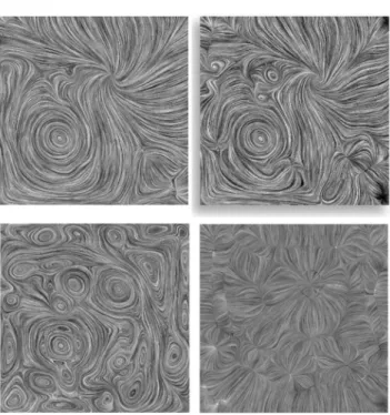
Yiying Tong USC Santiago Lombeyda Caltech Anil N. Hirani Caltech Mathieu Desbrun USCFigure 1: Decomposing Vector Fields: the tangential component of a wind field interacting with an ear (left, LIC visualization [5]) reveals its curl free component (middle) and divergence-free component (right) after decomposition. In this paper, simple computational tools are introduced to produce such a decomposition, for discrete 2D and 3D vector fields defined on irregular grids, even on curved manifolds.
Abstract
While 2D and 3D vector fields are ubiquitous in computational sci-ences, their use in graphics is often limited to regular grids, where computations are easily handled through finite-difference methods. In this paper, we propose a set of simple and accurate tools for the analysis of 3D discrete vector fields on arbitrary tetrahedral grids. We introduce a variational, multiscale decomposition of vec-tor fields into three intuitive components: a divergence-free part, a curl-free part, and a harmonic part. We show how our discrete ap-proach matches its well-known smooth analog, called the Helmotz-Hodge decomposition, and that the resulting computational tools have very intuitive geometric interpretation. We demonstrate the versatility of these tools in a series of applications, ranging from data visualization to fluid and deformable object simulation.
Keywords: Vector fields, Variational approaches, Hodge
decom-position, Scale-space description, Animation, Visualization
1
Introduction
Discrete multivalued fields such as vector and tensor fields are ubiq-uitous in computational sciences. In Computer Graphics, they are used in a large number of applications ranging from fluid and de-formable object simulation to the analysis of MRI data for medical prognosis. Due to the sheer complexity of these nonscalar fields, their numerical processing is most often performed on regular grids, due to a lack of simple and accurate tools for irregular grids. Yet, arbitrary grids are more efficient and flexible at discretizing 2D and 3D regions, whether they are in Euclidean spaces or on curved man-ifolds. The goal of this paper is to present a simple and accurate approach to vector field processing on arbitrary tetrahedral grids, to catalyze the development of algorithms and implementations of such rich data in computer graphics.
Most of the work done so far on discrete vector field analysis has tried to mimic well-known differential properties of vector fields dating back to Poincar´e (1854-1912). Globus et al. [11] for instance
described a methodology for vector field analysis by examining the eigenvalues of the jacobian matrix of a velocity field trilinearly in-terpolated on curvilinear grids. They also created a discrete topol-ogy of vector fields by connecting critical points through stream-lines. This notion of topology can be used to not only analyze, but also to describe vector fields, even noisy ones that can be smoothed while preserving [29] or simplifying [27,14] their topology. An al-ternative for computing the singularities of three dimensional flow fields was shown in [16] using Clifford algebra. It can not only find and classify point singularities, but also line and surface singulari-ties. However, the approach is so far restricted to regular grid data; moreover, the computations involved provide topological informa-tion only, and often return false positives. This is actually a com-mon problem: since most vector field feature detections are based on very local estimates (often using the jacobian or the winding number), inevitable noise in the data often leads to poor numerical quality of the approximants, and thus inaccurate feature detection. As we will see, we use instead a variational approach to offer a more global solution to feature detection that does not suffer from such sensitivity to noise.
Smoothing vector fields has also been proposed as an efficient way to simplify complex datasets, and render the analysis more tractable [29,4]: for instance, [24,9] use anisotropic nonlinear dif-fusion methods to clean “noise” (small-scale features) from 2D and 3D fluid flows. This general idea is essential when dealing with very complex data sets issued from large simulation on supercom-puters: the native resolution of the data prevents any global pro-cessing without prior simplification. We will also provide, in con-junction with a vector field decomposition, a multiscale description of vector fields to allow for a multiresolution probing of the data. 1.1 Hodge Decomposition for Smooth Fields For smooth data, there is a well known way to decompose a vec-tor field into both intuitive and useful components: it is called the Helmholtz-Hodge decomposition [1]. First, recall that∇= (∂/∂x,∂/∂y,∂/∂z)tis the gradient,∇·=∂/∂x+∂/∂y+∂/∂z is the divergence operator, and∇×is the curl operator (also called rota-tional). With this notation, for a smooth 3D vector fieldξdefined in a region
T
, there exists a unique decomposition satisfying the following properties:ξ=∇u+∇×v+h (1) where:
u is a scalar potential field; note that∇×(∇u) =0,
h is the so-called ”harmonic” vector field; note that∇·h=0 and
∇×h=0.
The uniqueness requires proper boundary conditions as well: ∇u must be normal to the boundary∂
T
ofT
, while∇×v must betan-gential to it. Due to the properties of the potential fields,∇u is called the curl-free component (∇×(∇u) =0), while∇×v is called
the divergence-free component (∇·(∇×v) =0). This decompo-sition is particularly interesting for extraction of the features and singularities of a flow. For instance, in 2D fields, the curl-free term
∇u contains only sources and sinks, while the divergence free term
∇×v contains only vortices (see Figure3). Therefore, in addition to the intrinsic mathematical values of this decomposition, these components correspond to our intuition about what is a flow.
This natural decomposition is, alas, only well defined for dif-ferential vector fields. One has to extend this smooth definition to the discrete setting for computational purposes, and this is no trivial matter as even the notion of divergence or curl needs to be properly defined for discrete data. Discrete Helmholtz-Hodge decomposition on regular grids has already been used in graph-ics (see [25,10] for instance) and is relatively straightforward to implement with a finite-difference approach. It is, however, much harder to design a practical and accurate method for arbitrary grids. Several mathematical methods have been proposed to solve this is-sue for piecewise-linear vector fields(see [3]). Recently, Polthier and Preuß have successfully derived a technique for 2D discrete piecewise-constant vector fields in [22,23]1that is particularly sim-ple to imsim-plement, and has the attractive feature of preserving most of the continuous properties of its differential counterpart. Thus, we propose to extend this technique to 3D, as well as combine it with a multiscale decomposition to provide a complete set of convenient tools for vector fields.
1.2 Outline and Contributions
In this paper, we first propose in Section2a discrete 3D Helmholtz-Hodge decomposition for irregular 3D grids, that both extends pre-vious work [22, 23, 25] and matches its well-known differential analog. Our projection of a vector field into three unique vector field components (a curl-free field, a divergence-free field and a harmonic field) preserves all the natural smooth properties in the discrete sense. In developing our discrete decomposition, we will introduce two discrete operators Div and Curl with definitions de-rived from a simple variational approach. These discrete versions of the smooth operators divergence and curl have intuitive physi-cal meaning that matches their smooth counterparts. We then in-troduce in Section3a multiscale representation of the projected 1Another attempt to define such a decomposition was also proposed in [26], but in a different context.
Figure 2: Piecewise-constant Vector Fields: A 3D example of a vec-tor field used in a scientific simulation; the vecvec-tor field is assumed constant within each tetrahedron.
fields, where fine-scale details are successively suppressed while main features are preserved. Such a hierarchical decomposition is particularly interesting for visualization purposes, as complex flows can be represented at multiple scales to heighten the user’s intuition and understanding of the global and local phenomena present in the data. The resulting multiscale vector field decomposition is a versatile computational tool: several applications are discussed and demonstrated in Section4, from a vector field processing and visu-alization toolbox, to the animation of fluids and elastic objects on irregular grids.
2
3D Vector Field Decomposition
In this section, we introduce a discrete vector field decomposition that guarantees a proper and unique separation of a discrete vec-tor field into a curl-free, a divergence-free and a harmonic field. We show that this discrete treatment closely parallels the smooth Helmholtz-Hodge decomposition (described in Section1.1), pre-serving all the fundamental differential properties while resulting in a very simple implementation. Moreover, the geometric inter-pretations behind each of the different step of this technique are simple and intuitive.
2.1 Setup and Definitions
Our basic setup is largely inspired by [23], and extended to 3D vec-tor fields.
Domain The finite domain on which the vector analysis needs to be performed is given in the form of a tetrahedralization
T
. We will make no assumption on the shape of the tetrahedra, or on the genus of the region: they can be arbitrary. However, for clarity’s sake, we will assume in this section that our domain is a region of the “flat” 3D (Euclidean) space. It will be shown later (in Section4.2.2) how straightforward it is to extend our discrete Helmholtz-Hodge decomposition to arbitrary embedding (for 3D volumes embedded in nD, as in space-time simulations for instance).Discrete Vector Fields On this domain, we will assume the input discrete vector fieldξto be cell-centered: inside each tetrahe-dron Tkof the domain, the vector field is supposed to be constant, and is represented by a vectorξk. If the input vector field is not cell-centered (as in finite element computations for instance), the field can be averaged over each tetrahedron or simply sampled at the barycenter to create the appropriate cell-centered representation.
Discrete Potential Fields Our goal is to mimic the smooth Hodge decomposition. We thus need to define two potentials (resp. u and v) such that their derivatives (resp. gradient and curl) repre-sent the curl-free and divergence-free components of an input field ξ. Given our choice of input vector fields, it is natural to define these potential fields as being linear on each tetrahedron of
T
, i.e., defined at vertices (also called nodes) of the domain and linearly in-terpolated within each tetrahedron. The gradient or the curl of any node-based linear function will then be constant within any given tetrahedron, defining a proper cell-centered vector field. Notice that this is reminiscent of the staggered grid approach commonly used for regular grids [25] due to its superior numerical qualities: the vector field and the potentials are not collocated, but instead, live on dual grids. In our case, the primal potential field defined using linear finite elements naturally induces a dual vector field, constant in each grid cell. This is also the traditional setup of what is some-times called the mixed finite-volume/finite-element method [17].Definitions In order to avoid confusion, we will always use the index i to refer to a node of the tetrahedralization
T
at a spatial position xiand use the index k for a tetrahedron Tk∈T
. We now define the function spaces we will be working with.We will call
L
the (primal) space of piecewise-linear potential fields. A potential (scalar or vector) field f∈L
is expressed as:f(x) =
∑
i
φi(x)fi,
withφibeing the piecewise-linear basis function valued 1 at node
xi, and 0 at all other nodes of
T
, and fibeing the value of f atxi. Due to the local support of the basis functionsφi, the value of f within a tetrahedron defined by(xi1,xi2,xi3,xi4)is simply: f=φi1fi1+φi2fi2+φi3fi3+φi4fi4. We will also use the notation
φikto refer to the functionφirestricted to tetrahedron Tk.
We will call
C
the (dual) space of piecewise-constant vec-tor fields. A vector field w∈C
can expressed as: w(x) =∑kψk(x)wk, withψkbeing the piecewise-constant basis function valued 1 inside tetrahedron Tkand 0 anywhere else. The vector field w is therefore valued wkinside the tetrahedron Tk. Notice that both the gradient (resp. the curl) of a primal scalar (resp. vector) potential field in
L
is a dual vector field, i.e., a member ofC
, since a piecewise-linear field has piecewise-constant first derivatives.The discrete vector field decomposition we present next can therefore be formulated as follows:
For a vector fieldξ∈
C
, find the two potential fields u∈L
and v∈L
, and the vector field h∈C
, such that a Hodge-type decomposition (Eq.1) can be formulated forξ.Next, we define the discrete notions of divergence-free and curl-free components of a vector field, and propose a discrete decom-position that satisfies the uniqueness property for proper boundary conditions.
2.2 Curl-free Component
Using the smooth Hodge decomposition as a guide, we wish to find a piecewise-linear function u such that its spatial gradient∇u cap-tures the curl-free part of the original vector fieldξ. In the smooth case, this component corresponds to the L2projection ofξonto the space of curl-free fields [1]. Therefore a natural, globally-optimal field u satisfying this property can be defined as minimizing the fol-lowing quadratic functional [23]:
F(u) =1 2
T(∇u−ξ)
2dV (2)
A necessary condition for a potential u to be a minimizer of this function is to satisfy, for each node i, the linear equation
∂F(u)/∂ui=0. In the AppendixA, we show that these linear equa-tions can be expressed as:
∀i,
T∇φi·∇u dV=
T∇φi·ξdV. (3)
2.2.1 Solving for the Potential
The optimality conditions being linear, it is straightforward to find the potential u by solving the linear system in Eq.3, which can be rewritten at each node as a simple sum over the neighboring tets:
∀i,
∑
Tk∈N(i)
∇φik·(∇u)k|Tk|=
∑
Tk∈N(i)∇φik·ξk|Tk| (4) where
N
(i)is the set of all tetrahedra immediately adjacent to the node i, and|Tk|is the volume of tetrahedron Tk. The locality of these conditions leads to a sparse matrix. Forming this matrix is a simple matter of computing the non-zero coefficients involved; rewriting(∇u)kas a function of the local basis functions indicates that these coefficients are of the form∇φik·∇φjk. To facilitate the implementation, we note that∇φikis simply the vector orthogonal to the face fikopposite to i in the tet Tk, pointing towards i and with a magnitude of|∇φik|= area3|(Tkfik|). Using this geometric definitionFigure 3: Vector Field Decomposition (visualized using LIC [5]): a 2D field (top, left) is decomposed into its curl-free part (middle, left) and its divergence-free part (bottom, left). Right: the same de-composition after a non-linear smoothing of the potentials. Notice that only the small vortices have disappeared as can be seen from the superimposed features (top).
of the terms involved, the coefficients of the matrix of this linear system can then be computed easily.
To guarantee uniqueness we also need to specify boundary con-ditions. We choose to set u|∂T =0: this results in∇u being orthog-onal to each face on the boundary which is a required condition for uniqueness in the smooth Hodge decomposition [1]. Notice that any other constant value at the boundary could be used, reflecting the fact that the potential u is defined up to a constant. Given these boundary conditions the sparse linear system can now be solved efficiently using a conventional conjugate gradient technique.
2.2.2 Discrete Divergence
Eq. (3) suggests the introduction of a discrete operator Div. For a vector field w∈
C
and a node xi, we define:(Div w)(xi) =
∑
Tk∈N(i)
∇φik·w|Tk|. (5) Indeed, with this definition, Eq.4can be directly expressed as a discrete equivalent of the Poisson equation:
Div(∇u) =Divξ. (6)
Notice that in the smooth case, u satisfies the same Poisson equa-tion, but with the smooth divergence operator∇·, as can be seen by
applying∇·to both sides of Eq. 1. Note also that Div(∇u)is the discrete Laplacian defined for 2D in [20], and for 3D in [18]: our operator is therefore in agreement with previous work, as already noticed for the 2D case in [22,21].
The Div operator defined in Eq. (5) has a very natural physical interpretation, similar to the 2D formula found in [23]: since the gradient inside a tet of a node’s linear basis function is orthogonal to the opposite face (see Section2.2.1), this operator simply sums the “flux” of the vector field through the one-ring region around a vertex. Additionally, in AppendixCwe prove that Div(∇×w) =0 for any vector field w∈
L
. Thus Div satisfies an identity analogous to a vector calculus identity satisfied by the usual divergence oper-ator. All these analogies with the differential divergence operator justify the name Div for this discrete operator.2.3 Divergence-free Component
Still keeping the smooth Hodge decomposition in mind for guid-ance, we now wish to find a piecewise-linear node-based vector field v such that its curl captures the divergence-free part of the original vector fieldξ. Following the differential definition of∇×v
as being the L2projection ofξonto the space of divergence-free fields, we define an energy G as:
G(v) =1
2
T(∇×v−ξ)
2dV (7)
The divergence-free component∇×v ofξcan now be defined as the minimizer of this quadratic functional. The global critical point of G must satisfy the following linear equations, as proven in AppendixB: ∀i, T∇φi×(∇×v)dV= T∇φi×ξdV (8)
2.3.1 Solving for the Potential
The above optimality conditions can, once again, be written as a local sum over neighboring tetrahedra. Therefore, solving for v amounts to solve the sparse, linear system defined by:
∀i,
∑
Tk∈N(i)∇φik×(∇×v)k|Tk|=
∑
Tk∈N(i)∇φik×ξk|Tk|. (9) Since∇×(∑iφivi) =∑i(∇φi×vi), the non-zero coefficients of the matrix of this linear system are now related to the cross products
∇φik×∇φjk. Their evaluation is simple to perform using the geo-metric interpretation of∇φik(see Section2.2.1): it will reduce to a scaled version of the cross product between normals to two adjacent faces.
In the smooth case a sufficient boundary condition to ensure uniqueness of the Hodge decomposition is that the divergence-free part be tangential to the boundary. In our discrete setting, a suffi-cient condition to ensure this condition is that v|∂T =0 which
en-sures that∇×w is tangential to the boundary. Given these boundary
conditions the sparse linear system can be solved efficiently using a conventional conjugate gradient technique.
2.3.2 Discrete Curl
The condition in Eq. 9suggests the definition of a discrete Curl operator. For every w∈
C
and a given node xi, we define:(Curl w)(xi) =
∑
Tk∈N(i)
(∇φik×wk)|Tk| (10) Therefore, the critical point v of G satisfies the condition Curl(∇× v) =Curlξas in the smooth case. Notice, that, here again, this discrete equation is valid in the differential case: it corresponds to Eq. (1) after we apply the curl operator to each side of the equality.
This discrete Curl operator at a node xiis the volume-weighted sum of intuitive terms: each cross product within a tetrahedron rep-resents the vorticity of the component of the input vector field tan-gent to the face opposite to xi. This vorticity indicates the direction and magnitude of a small paddle wheel that would create this vec-tor field locally. Finally, we prove in AppendixCthat Curl(∇u) =0 for any scalar field u∈
L
. Again, this is the discrete analog of the corresponding identity from vector calculus, further justifying the name Curl for the discrete operator just defined.Figure 4: 3D Vector Field Decomposition: A 3D field (left, hedge-hog visualization) reveals very simple curl-free (middle) and divergence-free (right, line vortex) fields after processed by our dis-crete decomposition; in this particular case, the harmonic part is a large, almost constant vector field.
2.4 Complete Decomposition
Once the divergence-free part and the curl-free part have been uniquely defined, the original field can be uniquely rewritten as a sum of three components:ξ=∇u+∇×v+h, matching the smooth
Helmholtz-Hodge decomposition (Eq.1). The last cell-centered vector field h is easily found by subtracting∇u and∇×v from the
initial fieldξon a per-tetrahedron basis. This field h is traditionally called harmonic in the smooth case, as it is both divergence and curl free. Interestingly, this discrete vector field is also divergence-free and curl-divergence-free in the discrete sense. Indeed, if we apply our Div operator to Eq.1, we obtain Divξ=Div(∇u) +Div(h)since Div is linear and the discrete divergence of a rotational field is null as shown in AppendixC. Since u satisfies Eq.6at every node of the domain
T
, we conclude that Div h=0. Similarly, by apply-ing Curl to Eq.1, we obtain: Curl h=0. Thus, our decompositionsatisfies all the fundamental properties of the smooth Helmholtz-Hodge decomposition: our discrete operators are consistent with their smooth counterparts.
This discrete harmonic term h contains the non-integrable com-ponent of the field, i.e., the part that can not be expressed as deriving from potential fields: this corresponds to an incompressible, irrota-tional flow, and is often in practice a small or near constant vector field when fluid flows issued from fluid mechanics simulations are used. Notice however that this term can be rather large for flows on high-genus volumes.
Notice finally that our 3D results can also be used for 2D flows, but it then reduces to the 2D decomposition method proposed in [23], where the curl operator is particularly simpler (the curl is just a scalar in 2D, while it is a vector in 3D). We use this 2D de-composition in some of our figures to exemplify the characteristics of our decomposition, as it provides a much simpler visual under-standing.
Limitations Although the implementation of our method within a tet mesh library is straightforward, it is not without limitations. First, our decomposition requires solving a global, linear system. Conjugate gradient solvers with good preconditioners being readily available, this is not a numerical issue in practice (although the con-dition number of our linear system increases if the tets are degen-erated) as it only takes less than a second for a datasize of several thousand nodes. Nevertheless, this is more computationally inten-sive than a purely local method such as [11]. As already pointed out
Figure 5: Feature Detection and Smoothing. The leftmost vector field (visualized with LIC) is filtered linearly (middle): the small features do disappear, but the remaining ones have been significantly attenuated and displaced by the isotropic smoothing. On the other hand, our non-linear smoothing (right) does preserve the major features intact, while still removing the noise: this will provide a better scale-space. for 2D vector fields [22], there is however a significant advantage
in finding a varationally-motivated decomposition: the global na-ture of this approach makes it very robust to both the irregularity of the 3D mesh, and the vector field noise. Since all the main smooth properties are also preserved, we argue that the extra computational cost is well spent.
3
Multiscale Vector Field Description
While breaking down a discrete vector field into intuitive, simpler components is helpful, complex flows can however be overwhelm-ingly intricate with phenomena happening at all scales. For an ac-curate analysis and visualization of such flows, as well as for an efficient handling of their inherent complexity, we need to develop adequate tools that highlight the major phenomena present in the data. In this section, we propose a simple technique to provide a multiscale description of an arbitrary vector field to remedy this sit-uation, while being compatible with the previous decomposition. 3.1 Necessity of Multiscale Description
A visual depiction of complex vector fields often fails to convey the general “trend” of the flow at first sight: multiple tiny vortices or other local phenomena creates visual noise in the visualization of what could otherwise be a fairly steady flow. Macroscopic ma-nipulation of vector field data, for visualization for instance, can also be seriously impaired by the sheer size of data, even if ex-tremely small-scale phenomena are often not relevant. These issues are traditionally addressed by multiscale methods in graphics. Re-search in vision has been also focusing on the development, based on empirical studies of our visual system, of the closely-related no-tion of scale space [15] for object recognino-tion and segmentano-tion of images. In order to facilitate the analysis and visualization of com-plex vector fields, we present next a multiscale representation that helps separating small-scale phenomena from large-scale features. Combined with the discrete Hodge decomposition, this provides a powerful and intuitive tool for vector field analysis.
3.2 Smoothing Potential Fields
The key idea to obtain a multiscale representation is to perform fil-tering of the potentials, instead of the vector field itself as was done in [24,8,9,29,18,4]. Indeed, if we were to smooth the potential field u, its gradient would still represent a curl-free field, where the small scale sources and sinks would have been simply eliminated. Likewise, the curl of a smoothed out field v would always represent a divergence-free field, where only the large-scale vortices remains. Thus, we are consistent with the initial decomposition all along the smoothing process, preserving the fundamental decomposition of the flow even across scales.
Several smoothing techniques can be used for both potentials u and v. A linear scale-space [15] can be easily obtained by suc-cessive Laplace filtering of the potentials, as was proposed in [4]. However, significant reduction of amplitude may happen due to the linearity of the smoothing operator: small vortices do disappear during filtering, but large vortices decreases in magnitude and get shifted (see Figure5). To remedy this effect, non-linear filtering can be used instead as it better preserves salient features [9]. A large number of anisotropic and/or non-linear smoothing have been pro-posed, mostly following initial work in image processing by Perona and Malik [19]. Any of these smoothing techniques can be applied in our context [24,18]. In the next section, we focus on the two smoothing procedures we implemented.
3.3 Implementation
To create a linear scale-space, we perform independent Laplacian smoothing of both u and v, directly onto the irregular grid as in [6]. This smoothing operation can be done very efficiently as we can reuse the discrete Laplacian matrix we already set up for the dis-crete Hodge decomposition (see Section2.2). This amounts to a convolution of the potential fields by a Gaussian [4], eliminating the small variations of the potentials, which in turn eliminates the small features of the original field. Mathematically, we are simply integrating four diffusion equations:
∂u ∂t =ku∇ 2 u ∂vx ∂t =kv∇ 2v x ∂ vy ∂t =kv∇ 2v y ∂ vz ∂t =kv∇ 2v z
where kuand kvcan be chosen independently. The boundary condi-tions (u|∂T =0 and v|∂T =0) are maintained during the smoothing
to preserve the properties of the vector field decomposition. We also offer the option of creating a multiscale description of the flow by performing non-linear smoothing of u and v directly on the irregular grid too, using the methods developed in [8,18]. This can be done both in 2D and in 3D, and has the desired effect of smoothing out small-scale features fast while mostly preserving the large-scale phenomena as can be seen on Figure5. The implemen-tation is straightforward as this technique is also based on the same discrete Laplacian operator, additionally weighted locally to make the diffusion non-linear.
In practice, having both tools available is particularly useful: Laplacian filtering can suppress small details extremely fast in most flows without severely affecting the main features; there is however a noticeable shift in the features’ location due to the isotropic diffu-sion process, as demonstrated in Figure5. The non-linear filtering, on the other hand, is much needed when small-scale features with strong amplitude (such as small, but powerful vortices) are present,
as these features may be the main interest of the flow. It is, however, more time consuming (a factor of ten is often observed). Compared to previous smoothing techniques [9,4], what we presented in this section works conjunctly with the discrete decomposition, provid-ing an enhanced tool for vector field manipulation.
4
Applications and Results
The different computational tools we presented have a large vari-ety of applications in graphics. In this section, we show how the multiscale decomposition we propose and the discrete operators we derived are useful, with little or no extra work, for vector field pro-cessing, visualization, and even simulation.
4.1 Vector Field Processing Toolbox
With the multiscale decomposition described in the previous sec-tion, a vector field processing toolbox can easily be designed, by extending what was done for 3D geometry in [12]. Indeed, high frequencies can be eliminated through smoothing, but could also be extracted or even amplified. For instance, if ξ is smoothed into a new field ˆξ, the differenceξ−ξˆwill represent the details of the original signal. Simple linear combinations of this sort will allow us to extract and process any range of “frequencies” from ar-bitrary fields. Additionally, the Helmholtz-Hodge decomposition adds more degrees of freedom in the range of possible manipula-tion, since we can also target more specific signal components: at each scale, we have the divergence-free and the curl-free compo-nent. It is a straightforward operation to, for example, remove the small-scale divergence-free component of a discrete vector field. Similarly, our tools allows to resample a divergence-free vector field on a different grid, while preserving its divergence-free na-ture. We show vector field processing in Figure6where a field is enhanced, amplifying the amount turbulence initially present in the data.
Figure 6: Vector Field Processing: An initial flow (top left) is de-composed in divergence-free and curl-free components; these com-ponents are then enhanced (resp. bottom left and bottom right), and summed back to create a new, more turbulent flow (top right).
4.2 Visualization Toolbox
Visualization can be a very strong help in “understanding” a vec-tor field: van Wijk [28] for instance uses ink advection and decay to perturb an initial image according to the flow in a realtime 2D simulation/visualization, creating a very intuitive depiction of the flow characteristics. The conjunction of a multiscale description and a decomposition of the vector field that we presented makes for a very nice framework for developing additional visualization tools. In this section, we explore some basic visualization tools that we have implemented in our framework.
4.2.1 Feature Detection
A lot of work has been targeted at finding critical points of vector fields, as originally attempted in [11]. These critical points are of-ten classified depending on the eigenvalues of the matrix∇ξat a point in space. In our case, however, critical points of the flow can be found as critical points of the potentials as we describe next. No-tice that testing for critical points on potential fields (that have been found through a global, integral equation) is much less sensitive to noise in the data. We will therefore be less likely to get false pos-itives, a serious problem often observed in previous local methods (see [16] for instance).
Sink and Source Detection A sink corresponds to a local maximum of the potential u. Following what was done for 2D fields in [22], we define a vertex of
T
to be a local maximum if the value of u at that vertex is larger that the neighbors’ values of u. Conversely, a source is a local minimum, easy to define on a 3D irregular grid by simply exploring the 1-ring neighbors. Addition-ally, a larger support can be used, along with a threshold, to prune out all the minor details if needed. Figure5shows the sinks and sources for a given flow, and for its smoothed version.Vortex Detection Each vector in the potential v represents a direction of vorticity and an amplitude of the local vorticity. Very similarly, we can also define vortices as local extrema of the scalar field||v||. One can also detect the vortices in a given direction d by finding local maxima of the field v·d. Finally, one can track a
tube vortex (a curve around which a swirl is happening) by finding a local extremum in magnitude, then using the vorticity direction to track the piecewise-linear curve of maximum vorticity.
Higher-order features One could also find more complex fea-tures, such as saddles and spiral saddles (where there is a vortex in a plane, and a source in the orthogonal direction to the plane), by finding higher-order critical points of the two potentials u and
v. This idea, initially proposed by [23], can also be implemented rather simply in our context, as inflexion points and saddle points can be detected on discrete fields by local exploration again. Fur-ther work needs to be done to really provide the user with a whole catalog of features, analogous to the types defined by Abraham and Shaw [2].
4.2.2 Tangential 3D Vector Fields in Higher Space
Although we presented both our Helmholtz-Hodge decomposition and our multiscale representation for 3D vector fields in 3D, we can extend it to 3D vector fields living on a 3-manifold embedded in a higher dimensional space. The vector should be seen as living in the tangent space of this 3-manifold. All the derivations are still valid, as they were only using quantities intrinsic to the manifold. The only difference for the decomposition algorithm is that the bound-ary conditions have to changed to maintain uniqueness. However, just like in the 2D case [23], one can add the constraint that the vol-ume integral of the potentials u and v must be zero: this ensures a unique pair of potentials, and preserves the Helmholtz-Hodge de-composition qualities even for arbitrary embedding. Figure1shows the equivalent 2D decomposition for a surface embedded in 3D. The
3D equivalent can be used for space-time simulation, for example. Notice finally that the Laplacian smoothing turns into a Laplace-Beltrami smoothing for 3D non-flat manifolds, as previously used in [7]: we can therefore still build a space-scale easily even for these higher-dimensional cases. Developing feature-preserving al-gorithms for non-flat manifolds is however, still an active research theme.
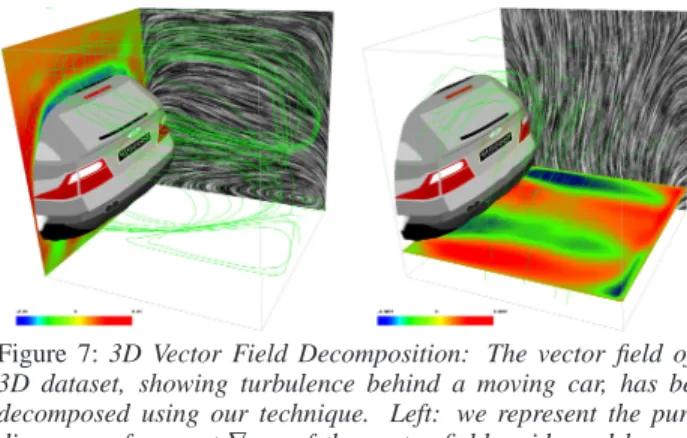
Figure 7: 3D Vector Field Decomposition: The vector field of a 3D dataset, showing turbulence behind a moving car, has been decomposed using our technique. Left: we represent the purely divergence-free part∇×v of the vector field, evidenced by
parti-cle tracing and a LIC cross-section of this component. Right: this time, the potential v is represented. The false color cross-sections represent the magnitudes of these fields.
4.3 Vector Fields for Animation
Our discrete 3D vector field decomposition also has applications in computer animation and simulation. We review a few connections we have explored so far.
Fluid Animation
One of the most recognizable features of most fluid flows is the presence of intricate swirls and complex turbulence. Fluid mechan-ics and recent work in computer graphmechan-ics have been able to obtain very convincing simulation when simulating incompressible fluids such as water. Keeping the flow divergence-free is essential in get-ting all the nice vortices we are accustomed to. As mentioned early on in this paper, most simulations use a projection to get rid of the curl-free components that may appear during simulation via a finite-difference approach on regular grids [25]. Similarly, preventing the damping of smoke vortices by detecting them and slightly increas-ing their energy has been proven important for the visual renderincreas-ing of flows [10]. Our approach allows to extend these routine proce-dures to arbitrary grids, opening the possibilities for adaptive sim-ulation: arbitrary boundaries and arbitrary refinements can not be easily dealt with regular grids, whereas arbitrary grids offer a much needed flexibility.
The previously-mentioned vector-field processing toolbox can also be use for “flow design” in animation: a given wind field can be edited and tweaked as wished using our computational tools. An animator can for instance sketch a vector field roughly, and our ma-chinery can turn this coarse field description into a purely vorticial field, even adding small details if necessary.
Animation of Deformable Objects
Linear elasticity is often used as a particularly simple model for formable object simulation. Internal forces are derived from the de-formation field, that is, from the displacements from the reference shape. In particular, in Debunne et al. [6] for instance, Hooke’s law is expressed as a linear combination of the Laplacian of the de-formation field∇2d, representing the propagation of deformation
(pure compression), and of the gradient of the divergence of the de-formation field,∇(∇·d), representing a volume-preserving force.
The numerical discretization of the Laplacian was exactly similar
to our discrete Laplacian (see Section2.2). A derivation of the sec-ond operator was also proposed, but the numerical quality was far below threshold compared to the Laplacian. Our novel operators introduced in this paper result in another discretization, fully com-patible with the Laplacian, therefore guaranteeing better numerical quality. Indeed, in the smooth as well as in the discrete case, the following identity holds:
∇(∇·w) =∇×(∇×w) +∇2w
This means that the volume preservation force can be computed using the Laplacian and the Curl operator we defined, providing a coherent set of operators. Notice finally that we do not need the full-blown decomposition, but only the local discrete operators we derived. We will exploit this application of Div and Curl for elas-ticity in a future paper.
5
Conclusion and Discussion
In this paper, we have developed a discrete multiscale vector field decomposition, along with a number of computational tools to ma-nipulate and analyze vector fields. The computations involved are very straightforward, and the properties exactly match the differen-tial analog known as the Helmholtz-Hodge decomposition. Further-more, the discrete operators developed along the way have a very intuitive justification, as well as a solid variational foundation. A scale-space can also be constructed by repeated smoothing, while preserving the initial decomposition across all scales. The result is a versatile, multi-purpose set of tools that can be used for several vector field processing applications, such as visualization, analysis, or even animation.
Future Work We plan on further exploring the visualization pos-sibilities of our decomposition. Using such a multiscale decompo-sition on animated vector fields also seems like a natural contin-uation of our work. Finally, our decomposition is tightly related to the more general field of differential forms and exterior calcu-lus [1,13], tying in nicely with the field of Clifford Algebra. We will also explore how our new results can be used in dynamics, for Lie derivatives for instance.
Acknowledgements The authors are extremely grateful to Peter Schr ¨oder for support, Konrad Polthier for inspiration, R ¨udiger Westerman for data, John McCorquodale for feedback, and Alain Bossavit and Melvin Leok for collaboration. This work was supported in part by the NSF (CCR-0133983, DMS-0221666, DMS-0221669, EEC-9529152).
References
[1] ABRAHAM, R., MARSDEN, J.,ANDRATIU, T., Eds. Manifolds, Tensor
Analysis, and Applications. Applied Mathematical Sciences Vol. 75,
Springer, 1988.
[2] ABRAHAM, R.,ANDSHAW, C., Eds. Dynamics: The Geometry of
Be-havior. Ariel Press (Santa Cruz, CA), 1984.
[3] AMROUCHE, C., BERNARDI, C., DAUGE, M.,ANDGIRAULT, V. Vector Potentials in Three-Dimensional Non-smooth Domains. Math. Meth.
Appl. Sci. 21 (1998), pp. 823–864.
[4] BAUER, D.,ANDPEIKERT, R.Vortex Tracking in Scale-Space.
Sympo-sium on Visualization (Joint Eurographics-IEEE TVCG) (2002).
[5] CABRAL, B.,ANDLEEDOM, L. C. Imaging Vector Fields Using Line Integral Convolution. In Proceedings of SIGGRAPH (1993), pp.263– 272.
[6] DEBUNNE, G., DESBRUN, M., CANI, M.-P.,ANDBARR, A. H. Dynamic Real-Time Deformations Using Space & Time Adaptive Sampling. In
Proceedings of ACM SIGGRAPH (August 2001), pp. 31–36.
[7] DESBRUN, M., MEYER, M., SCHRODER, P.,¨ ANDBARR, A. H. Implicit Fairing of Arbitrary Meshes using Diffusion and Curvature Flow. In
Proceedings of ACM SIGGRAPH (1999), pp. 317–324.
[8] DESBRUN, M., MEYER, M., SCHRODER, P.,¨ ANDBARR, A. H.Anisotropic Feature-Preserving Denoising of Height Fields and Bivariate Data. In
[9] DIEWALD, U., PREUER, T.,ANDRUMPF, M. Anisotropic Diffusion in Vector Field Visualization on Euclidean Domains and Surfaces. In
IEEE Trans. on Vis. and Computer Graphics (2000), pp. 139–149.
[10] FEDKIW, R., STAM, J.,ANDJENSEN, H. W.Visual Simulation of Smoke. In Proceedings of ACM SIGGRAPH (2001), pp. 23–30.
[11] GLOBUS, A., LEVIT, C.,ANDLASINSKI, T. A Tool for Visualizing the Topology of Three-Dimensional Vector Fields. In Proceedings of
IEEE Visualization (1991), pp. 33–40.
[12] GUSKOV, I., SWELDENS, W.,ANDSCHRODER, P.¨ Multiresolution Signal Processing for Meshes. In Proceedings of ACM SIGGRAPH (August 1999), pp. 325–334.
[13] HIRANI, A. N.Discrete Exterior Calculus. PhD thesis, Caltech, 2003.
[14] LEEUW, W. C. D.,ANDLIERE, R. V. Collapsing Flow Topology using Area Metrics. In Proceedings of Visualization (1999), pp. 349–354. [15] LINDEBERG, T. Scale-Space Theory: A Basic Tool for Analysing
Structures at Different Scales. Journal of Applied Statistics 21, 2
(1994), pp. 225–270.
[16] MANN, S.,ANDROCKWOOD, A.Computing Singularities of 3D Vector Fields with Geometric Algebra. In Proceedings of IEEE Visualization (2002), pp. 283–289.
[17] MCCORMICK, S. F.Multilevel Adaptive Methods for Partial Differen-tial Equations — Chapter 2: The Finite Volume Method, vol. 6. SIAM,
1989.
[18] MEYER, M., DESBRUN, M., SCHRODER, P.,¨ ANDBARR, A. H. Discrete Differential-Geometry Operators for Triangulated 2-Manifolds. In
Proceedings of VisMath (2002).
[19] PERONA, P.,ANDMALIK, J. Scale-space and Edge Detection using Anisotropic Diffusion. IEEE Transactions on Pattern Analysis and
Machine Intelligence 12, 7 (1990), pp. 629–639.
[20] PINKALL, U.,ANDPOLTHIER, K. Computing Discrete Minimal Sur-faces. Experimental Mathematics 2, 1 (1993), pp. 15–36.
[21] POLTHIER, K. Computational Aspects of Discrete Minimal Surfaces.
Proceedings of the Clay Summer School on Global Theory of Minimal Surfaces (Hass, Hoffman, Jaffe, Rosenberg, Schoen, and Wolf Editors)
(2002).
[22] POLTHIER, K.,ANDPREUSS, E. Variational Approach to Vector Field Decomposition. Scientific Visualization, Springer Verlag (Proc. of
Eu-rographics Workshop on Scientific Visualization) (2000).
[23] POLTHIER, K.,ANDPREUSS, E. Identifying Vector Fields Singularities using a Discrete Hodge Decomposition. Visualization and
Mathemat-ics III, Eds: H.C. Hege, K. Polthier, Springer Verlag (2002).
[24] PREUER, T.,ANDRUMPF, M. Anisotropic Nonlinear Diffusion in Flow Visualization. In Proceedings of Visualization (1999), pp. 325–332. [25] STAM, J. Stable fluids. In Proceedings of ACM SIGGRAPH (1999),
pp. 121–128.
[26] TAUBIN, G. Linear Anisotropic Mesh Filtering. Tech. Rep. IBM Re-serach Report RC2213, 2001.
[27] TRICOCHE, X., SCHEUERMANN, G.,ANDHAGEN, H. A Topology Sim-plification Method for 2D Vector Fields. In Proceedings of IEEE
Vi-sualization (2000), pp. 359–366.
[28] VANWIJK, J. J. Image-based Flow Visualization. In Proceedings of
ACM SIGGRAPH (2002), pp. 745–754.
[29] WESTERMANN, R., JOHNSON, C.,ANDERTL, T. A Level-set Method for Visualization. In Proceedings of Visualization (2000), pp. 147–154.
A
Divergence Operator
Below we derive the necessary conditions for a discrete, piecewise-linear scalar potential field u to be the unique minimum of the quadratic energy:
F(u) =1
2
T(∇u−ξ)
2dV
Using basic calculus and the fact that u(x) =∑iφi(x)ui, we can write: ∀i, ∂F(u) ∂ui = T d∇u dui (∇ u−ξ)dV (11) = T∇φi· dui dui(∇ u−ξ)dV (12) = T∇φi·(∇u−ξ)dV (13)
Therefore the condition for u to be a critical point of F is:
∂F(u)
∂ui =
T∇φi·(∇u−ξ)dV = 0
This integral can now be rewritten as a direct sum over the tetrahedra di-rectly adjacent to the node i, since∇φiis 0 everywhere else. Since∇u and ξare constant inside each tetrahedron, Eq. (3) is thus easily verified, as well as the correct expression for the discrete divergence operator Div.
B
Curl Operator
Now we derive the conditions for a discrete, piecewise-linear vector poten-tial field v to be the unique minimum of the quadratic energy:
G(v) =1 2
T(∇×v−ξ)
2dV
Using basic calculus and the fact that v(x) =∑iφi(x)vi, we can write: ∀i, dG(v) dvi = T d∇×v dvi (∇× v−ξ)dV (14) = T∇φi× dvi dvi(∇× v−ξ)dV (15) = T∇φi×(∇×v−ξ)dV (16)
where we also used the fact that, for any constant vector viand for an
arbi-trary functionφi,∇×(φivi) =∇φi×vi. Finally, the necessary condition of
minimality for G is simply:
dG(v)
dvi =
T∇φi×(∇×v−ξ)dV = 0
Here again, since∇φiis 0 everywhere except on the tetrahedra adjacent to
the node i, and since∇×v andξare constant inside each tetrahedron, we directly get Eq.8, which in turn leads to the natural definition of the discrete curl operator Curl.
C
Discrete Calculus Identities
Here we show that, away from the boundary, the discrete operators Div and Curl satisfy the following identities as in smooth vector calculus :
Div(∇×v) =0 (17) Curl(∇u) =0 (18) where u∈L and v∈L are piecewise linear scalar and vector fields
a b
e
f in the domainT. First we need a simple result about volumes of tetrahedra. For a tetrahedron T let a,b be 2 of its vertices and let e be the edge
vector that does not contain these vertices, ori-ented along the direction∇φa×∇φb. Then:
|T|∇φa×∇φb=
e 6.
To see this let f be the face opposite to a,θethe dihedral angle at edge e, and ha,hbthe heights of vertices a and b above their respective opposite faces.
Then |T|∇φa×∇φb= 1 3area(f)ha 1 ha 1 hb sinθe e ||e||= e 6. Now to prove (17) note that for any node xp:
(Div(∇×v))(xp) =
∑
Tk∈N(p) ∇φpk·(∇×v)k|Tk|=∑
Tk∈N(p) ∇φpk·∑
i∈Tk ∇φik×vi |Tk| =∑
Tk∈N(p)i∑
∈Tk vi·(∇φpk×∇φik)|Tk|=∑
Tk∈N(p)i∑
∈Tk vi· eip 6 .The third equality is from a basic identity about scalar triple products and the last one is from the result about tetrahedral volume derived above. This resulting sum is null. Indeed, for each vertex i neighbor of p, the oriented edges eipare opposite to the edge ip, and they form a closed loop around the
edge ip: their sum is therefore zero. To prove (18) we use similar reasoning and show that:
(Curl(∇u))(xp) =
![Figure 3: Vector Field Decomposition (visualized using LIC [5]):](https://thumb-us.123doks.com/thumbv2/123dok_us/1354672.2681250/3.918.68.835.77.1077/figure-vector-field-decomposition-visualized-using-lic.webp)