Wayne State University Dissertations
1-2-2013
Advanced Optimization Techniques For Monte
Carlo Simulation On Graphics Processing Units
Eyad Hailat
Wayne State University,Follow this and additional works at:
http://digitalcommons.wayne.edu/oa_dissertations
Part of the
Chemical Engineering Commons, and the
Computer Sciences Commons
This Open Access Dissertation is brought to you for free and open access by DigitalCommons@WayneState. It has been accepted for inclusion in Wayne State University Dissertations by an authorized administrator of DigitalCommons@WayneState.
Recommended Citation
Hailat, Eyad, "Advanced Optimization Techniques For Monte Carlo Simulation On Graphics Processing Units" (2013).Wayne State University Dissertations.Paper 766.
ADVANCED OPTIMIZATION TECHNIQUES FOR MONTE
CARLO SIMULATION ON GRAPHICS PROCESSING
UNITS
by
EYAD HAILAT DISSERTATION
Submitted to the Graduate School of Wayne State University,
Detroit, Michigan
in partial fulfillment of the requirements for the degree of
DOCTOR OF PHILOSOPHY 2013
MAJOR: COMPUTER SCIENCE Approved by:
Eyad Hailat 2013
All Rights Reserved
DEDICATION
Dedicated to my parents, Majed Hailat and Amal Alshouha. To my wife, Maram,
and to my little angel, Lilian. Also, I dedicate this work to my brothers and sisters
and their families. Special thanks to all my friends.
First, I would like to thank God almighty for giving me the chance to start and finish my Ph.D. and for all other good things happened to me in my life. Also, I am deeply grateful to my advisor, Dr. Loren Schwiebert for all the help and guidance during my Ph.D. study from day one. It is with his guidance, mentoring, and help the journey through graduate school was possible.
In addition, I would like to thank Dr. Jeffery Potoff, Dr. Hongwei Zhang and Dr. Weisong Shi for serving on my dissertation defense committee.
TABLE OF CONTENTS
Dedication . . . ii
Acknowledgments . . . iii
List of Tables . . . vii
List of Figures . . . viii
Chapter 1: Introduction . . . 1
1.1 Motivation . . . 1
1.2 GPU Architecture . . . 2
1.3 Structure of Fermi cards . . . 3
1.4 CUDA Review . . . 6
1.4.1 Synchronization and Concurrency . . . 7
1.4.2 Kernel Launch Specifications . . . 8
1.4.3 CUDA Memory . . . 9
1.4.4 CPU-GPU Communication . . . 9
1.4.5 Atomic Instructions on Global Memory . . . 10
1.4.6 Memory Coalescing . . . 10
1.5 CUDA Streams . . . 10
1.6 Monte Carlo Simulations . . . 12
1.7 Random Number Generator . . . 14
1.8 Other Applications of this Work . . . 15
Chapter 2: Related Work . . . 16
2.1 General Purpose GPU Programming . . . 16
2.2 Monte Carlo Simulations . . . 16
Chapter 3: Porting Canonical Ensemble to the GPU . . . 23
3.1 Markov Chain Monte Carlo Simulations . . . 23
3.1.1 Metropolis Method and Thermodynamic Ensembles . . . 23
3.1.2 Lennard-Jones Potential . . . 25
3.2 Structure of the Code . . . 25
3.3 Optimizing the canonical ensemble method for the GPU . . . 29
3.3.1 The block size effect . . . 29
3.3.2 The use of pinned memory . . . 30
3.3.3 The use of different GPU memory types . . . 30
3.3.4 Memory coalescing for fetching particle positions . . . 31
3.3.5 Loop unrolling technique in finding total energy . . . 31
3.3.6 Load balancing among threads and contributing particles . . . 34
3.3.7 Atomic operations on global memory transactions . . . 35
3.3.8 Block synchronization through global memory and atomic operations . . . 35
3.3.9 Numerical optimizations: tricks and tweaks . . . 35
3.4 Using cell list structure . . . 37
3.5 Results and Discussion . . . 39
Chapter 4: Grand Canonical Ensemble: One Simulation Box and a Reservoir . . . 50
4.1 MC Simulation for the Grand Canonical . . . 51
4.2 Parallel Algorithm and Implementation Details . . . 52
4.2.1 Implementation without Cell List . . . 53
4.2.2 Cell List Implementation . . . 55
4.2.3 Assigning Cells to Blocks . . . 60
4.2.4 Assigning Threads to Particles . . . 62
4.2.5 Adding Cell List Implementation to the Parallel Grand Canonical Algorithm . . . . 62
4.3 Performance Results . . . 62
Chapter 5: Gibbs Ensemble: Two Simulation Boxes . . . 69
5.1 MC Simulation of the Gibbs Ensemble . . . 69
5.2 Method . . . 71
5.3 Results and Discussion . . . 76
Chapter 6: Configurational Bias Gibbs Ensemble . . . 82
6.1 Introduction . . . 82
6.2 CBGEMC Method and Implementation . . . 83
6.3 Results and Discussion . . . 87
Chapter 7: Conclusion and Future work . . . 100
References . . . 103
Abstract . . . 115
Autobiographical Statement . . . 117
Table 3.1: Thread hierarchy and properties. . . 30
Table 3.2: Average program execution times (in seconds) and speedup overTowhee. . . 40
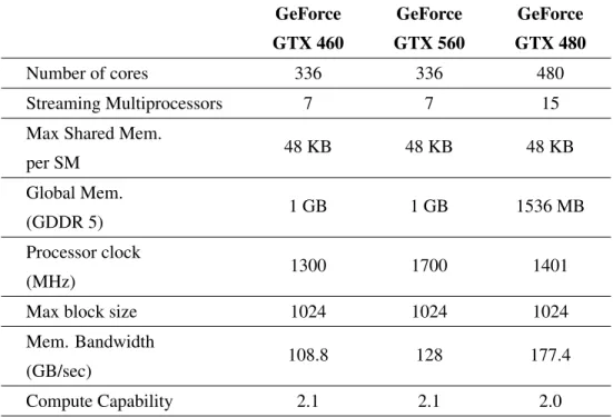
Table 3.3: Specifications for the three graphic cards used to run reported experiments. . . 41
Table 3.4: Desktop computers used for the experiments. . . 42
Table 3.5: Large vs. small block size and system performance. Numbers shown are speedup. . 44
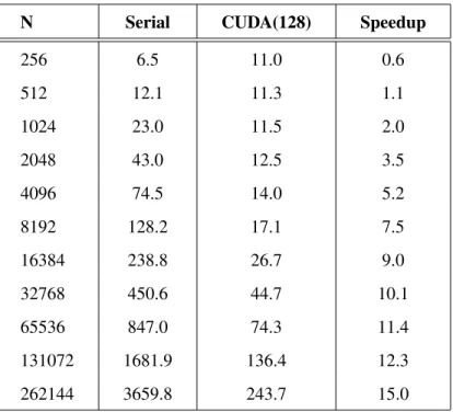
Table 3.6: CUDA vs Serial results on GTX 480 . . . 47
Table 3.7: Results of different cell list models . . . 48
Table 3.8: Speedup of cell list for a million steps . . . 48
Table 4.1: Execution times in seconds for different algorithm implementations. . . 64
Table 4.2: Legend of blocks, cells, and threads per kernel call. . . 64
Table 4.3: Different block sizes have different effect on resource utilization. . . 66
Table 4.4: Speedup of different cell list implementations over no cell list CUDA code. . . 67
Table 5.1: A comparison of a high and a low end GPU . . . 76
Table 5.2: A comparison of a high and a low end CPU . . . 77
Table 5.3: Execution times in seconds and speedup using the icc compiler. . . 78
Table 5.4: Execution times in seconds and speedup using the gcc compiler. . . 78
Table 6.1: Execution times in seconds for CB for different number of CB trials (K). . . 90
Table 6.2: Execution times in seconds for CB for different number of CB trials (K). . . 91
Table 6.3: Execution time in seconds of running simulations with 131072 particles in parallel. 92 Table 6.4: Speedup of running simulations with 131072 particles. . . 93
Table 6.5: Results for CB for different number of CB trials (K) in parallel. . . 96
LIST OF FIGURES
Figure 1.1: Fermi Memory Structure . . . 4
Figure 1.2: A grid structure . . . 5
Figure 3.1: A particle displacement attempt in Metropolis Monte Carlo method. . . 24
Figure 3.2: MC Simulation for the canonical method flowchart. . . 28
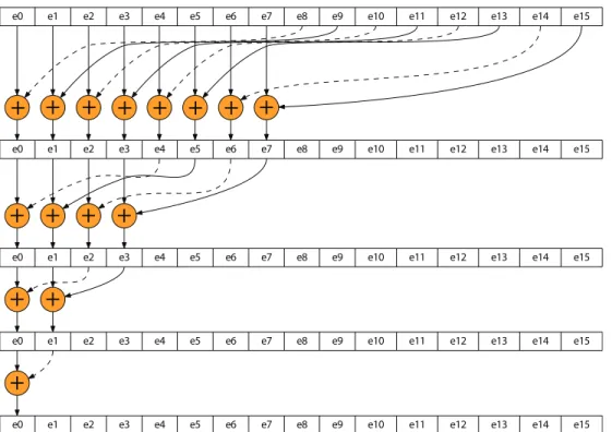
Figure 3.3: Calculating the partial sum in shared memory that use adjacent memory locations. . 32
Figure 3.4: Mapping algorithm for work load balancing across threads. . . 34
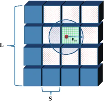
Figure 3.5: The volume is decomposed into cells. . . 38
Figure 3.6: Cell with all 26 adjacent cells. . . 39
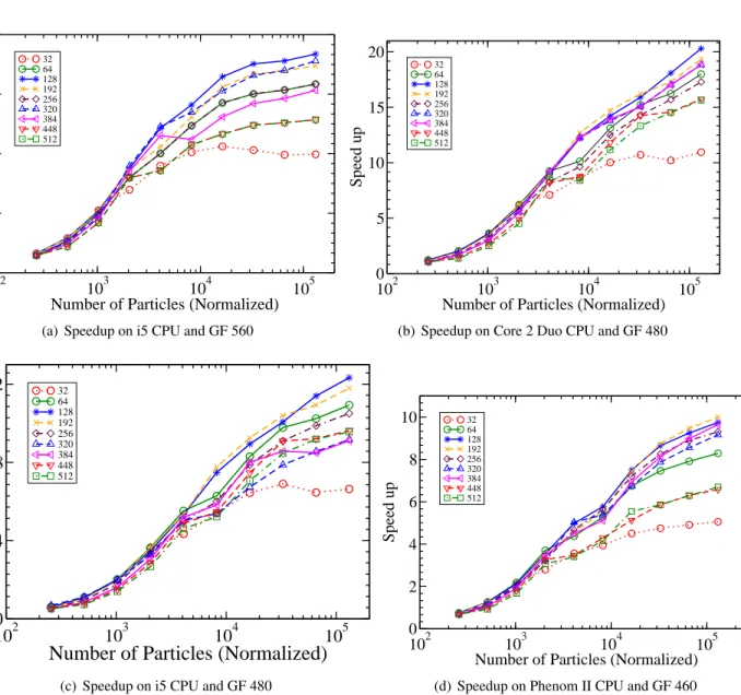
Figure 3.7: Plots of speedup for different block sizes on different platforms. . . 45
Figure 3.8: Developed serial code vs. Towheeelapsed times (logarithmic normalization). . . . 46
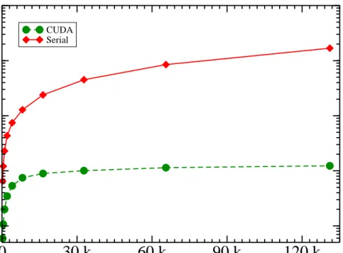
Figure 3.9: Serial vs. CUDA execution times for MC simulation on i5 and GeForce 480. . . 46
Figure 3.10: Execution times on two different platforms with GTX 480. . . 47
Figure 3.11: Different cell list implementations speedup . . . 49
Figure 4.1: Different methods in assigning cells to thread blocks . . . 59
Figure 4.2: Speedup of different algorithms . . . 65
Figure 4.3: Speedup of CUDA code with different cell list codes over CUDA with no cell list. . 66
Figure 4.4: Execution times for different algorithms with CUDA cell list. . . 67
Figure 4.5: Cell size and speedup. of particles per cell per thread forN = 262144. . . 68
Figure 5.1: An illustration of the three move types for the Gibbs ensemble method. . . 70
Figure 5.2: Execution time for the serial and the CUDA code . . . 79
Figure 5.3: The actual speedup and theoretical speedup of the CUDA code . . . 80
Figure 6.1: Particle transfer move with CB and K equals five. . . 85
Figure 6.2: Timeline of particle transfer in CB execution using K-1 independent streams. . . . 85
Figure 6.3: Vapor-liquid coexistence curves for Lennard-Jones fluid. . . 88
Figure 6.4: Histogram sampling the distribution of the gas and liquid phases . . . 89
Figure 6.6: Execution times of CUDA code on GTX 480 and K20c for large systems . . . 95
Figure 6.7: Execution time for parallel code with only particle transfer move . . . 97
Figure 6.8: Speedup for parallel code with streams. . . 98
1
CHAPTER 1
Introduction
1.1
Motivation
Graphics devices were introduced originally for entertainment. The first graphics processing unit was invented by NVIDIA in 1999 for creating game objects in real-time [106]. Since then, graphics units kept evolving to provide a huge amount of processing power that later was extended to do non-graphics applica-tions such as floating point operaapplica-tions and developed a high level set of shading languages such as DirectX, OpenGL, and Cg.
When GPUs first started using APIs for non-graphics purposes, they were called General Purpose Graph-ics Processing Units (GPGPU), showing good speedups over other methods. In that era, efforts were spent on utilizing vertex coordinates, texture, and shader programs, which was one drawback of using GPUs for general purpose computing. Another drawback to using the early GPUs for scientific applications is the need for an extensive knowledge of graphics APIs and the GPU architecture itself. Moreover, the lack for even the most basic programming features and operations such as random access to memory for reads and writes, double precision floating point operations, and operations on integer numbers were major reasons for not us-ing GPUs in many applications and considered limitus-ing factors. Later, programmus-ing with graphics APIs was replaced with parallel programming languages. Examples of high level parallel programming languages are BrookGPU [15] used for AMD GPUs, Open Computing Language (OpenCL) [120, 82], which is portable between GPU architectures, CUDA [55, 87], which is limited to be used on NVIDIA cards, and BSGP [52]. In addition, Chapel, developed by Cray Inc. [21] is an open source, portable parallel programming language that can be used on commodity clusters or desktop multicore systems.
Although OpenCL and CUDA provide different programming interfaces, they offer similar features. However, OpenCL is designed for a very general architecture; it can be used to program CPUs, GPUs, Digital Signal Processors (DSPs) and other devices from other vendors. This portability came with a price that affects the performance of OpenCL codes. In a performance comparison conducted in [59] between CUDA and NVIDIA’s OpenCL implementation, the study shows that CUDA performs better in terms of kernel
execution and memory transfer from and to the GPU running almost the same code. In addition, several differences in using both architectures are reported. One main difference between these two languages is that OpenCL can be compiled at runtime, which would slow down the overall execution time of the code. This technique allows the compiler to generate code on the fly targeting a specific GPU architecture. CUDA, on the other hand, does not have this concern since it is designed specifically for a single architecture. Other differences in the two APIs include context creation, mapping kernels to the GPU, and memory copying. See [82] for a complete API reference for programming with OpenCL.
1.2
GPU Architecture
Here we will discussGraphics Processing Units in terms of the architecture and its relationship with
the rest of the computer system. Also, we will mention the difficulties that may confront anyone who is interested in utilizing these devices [44, 72, 83, 50, 51].
Even if we can add more transistors to a chip, we cannot scale their voltage like we used to, and we cannot clock these transistors as fast. One solution is to run in parallel. With current GPU technology we can easily get a device loaded with hundreds of processors, and the future trend is even more. So, one should start thinking in parallel and start developing applications without thinking of the serial algorithm first.
There are some weak points for GPUs compared to CPUs in terms of architecture. Examples include that GPUs devote more transistors to arithmetic logic units and less to caches and control prediction in compari-son to CPUs. On the other hand, threads in GPUs are considered fine-grained and without expensive context switching like CPU threads. Individual GPU threads are considered to have poor performance compared to CPU threads, but thousands can run simultaneously. Moreover, GPUs have higher memory bandwidth.
Lately, tools have been developed to make the programmer’s parallel experience easier. IDEs such as Eclipse, NetBeans, and MS Visual Studio started to allow for integrating parallel programming lan-guages. Also, debugging tools for GPU code started to appear after developing the latest architecture, such as CUDA-GDB and Parallel Nsight for different Linux operating systems, and MS Visual Studio integration for Windows operating systems. In addition, other tools appeared such as Glift, a data structure framework that implements a set of structures that aims to simplify algorithmic development using GPUs. Structures implemented in Glift include a stack, quadtree, and octree [68]; more tools can be found in [53, 115, 116].
3
In addition, GPU computing became mainstream with the launches of MS Windows 7 and Apple Snow Leopard, so that the GPU will be accessible to any application as a parallel processor, not only as a graphics processor.
The host program performs all memory management,thread synchronization, and other setup tasks and then calls GPU kernels to perform the simulation. Examples of CUDA enabled devices are the GeForce 6 series GPU, their architecture description can be found here [60], and Tesla graphic cards [69].
1.3
Structure of Fermi cards
In June 2008, NVIDIA released a major revision to their architecture. Graphics cards like GeForce GTX 280, Quadro FX 5800, and Tesla T10, were the first cards to have the new unified hardware generation of GT200. This major revision has many updates over the previous one, such as increasing the number of streaming processor cores to almost double. Each register file was also doubled in size. In addition, there is better memory access coalescing that improves memory access efficiency for huge amounts of data. More-over, double precision floating point support was enhanced to support high performance scientific computing.
This NVIDIA generation of CUDA Compute and Graphics architecture is calledFermi.
The structure of a graphic card’s memory is different from any other device, as seen in figure 1.1. Fermi structure is different from serial processor’s memory and older graphic cards. There are two lines of eight Streaming multiprocessors (SMs) around one L2 cache. A host interface connects the GPU to the CPU via a PCI-Express interface. Each SM, see figure 1.2, has 32 cores. Each has a fully pipelined integer arithmetic logic unit (ALU) and floating point unit (FPU). One CUDA core executes a floating point or integer instruction per clock for a thread.
This memory model was adopted to take the advantage of different threads running the same code. A
thread is identified by athreadIdxthat consists of three coordinates inside the block: threadIdx.x,
threadIdx.y, and threadIdx.z that define the x, y, and z coordinates, respectively. On current GPUs, a block can contain up to 1024 threads for x- or y-dimension in compute capability 2.0 and 512 for earlier compute capabilities, and 64 threads for the z-dimension for any compute capability. On the grid level,
a three-dimensional grid of blocks is defined referencing the block by blockIdx.x,blockIdx.y, and
Figure 1.1: Fermi Memory Structure
afterward, shared by all threads in that block, and are accessed only inside kernels. The number of blocks in a
grid on one of the two dimensions can vary between one and 65,536, and are saved in variablesgridDim.x
andgridDim.yfor the x- and y-coordinate, respectively.
The Fermi memory hierarchy, shown in figure 1.1, illustrates that a thread can use both shared memory
and cache. This depends on the nature of the problem. The advantage of this memory model is scalability
of blocks. A programmer may have a limit on the number of threads in different GPUs but the number of blocks makes it more scalable.
For example, in the code portion below
Listing 1.1: Legal code portion of CUDA kernel launch
dim3 B l o c k S i z e ( 3 , 3 , 2 ) ; dim3 G r i d S i z e ( 6 , 4 , 1 ) ;
L a u n c h K e r n e l<<<G r i d S i z e , B l o c k S i z e>>>( p a r a m e t e r s ) ;
5
block is three dimensional block with a total of3×3×2 = 18threads per block, this makes it a total of
24×18 = 432threads that launch this kernel. On the other hand, a code portion like the listing below (1.2) cannot be executed since the number of threads exceeds the allowed number of threads.
Listing 1.2: Illegal code portion of CUDA kernel launch
dim3 B l o c k S i z e ( 3 2 , 3 2 , 2 ) ; dim3 G r i d S i z e ( 6 , 4 , 1 ) ;
L a u n c h K e r n e l<<<G r i d S i z e , B l o c k S i z e>>>( p a r a m e t e r s ) ;
It is a design decision on how to choose block size. To illustrate, if the number of threads is divided among more blocks, the total number of threads would be the same, but may have a disadvantage of extra overhead when trying to synchronize between blocks through global memory instead on synchronizing in shared memory in the case of working with threads in one block. In addition, there is a limit on the number of blocks that can run concurrently on any SM. In our study we have examined this factor on the system behavior. We study the performance when changing block size for the Canonical Ensemble method.
1.4
CUDA Review
Invented by NVIDIA, theCompute Unified Device Architecture(CUDA) parallel computing architecture
is now shipped in most NVIDIA graphic cards. This architecture is a hardware and software platform that defines the programming model, memory model, and execution model for issuing and managing computa-tions on GPUs, where the programmer does not need to directly map computacomputa-tions to the graphics pipeline. Compared to previously used graphics languages such as OpenGL and Cg, this architecture is implemented over the C language, which makes the process of developing GPU-based software for scientific computing a much easier job. Basically, CUDA facilitates heterogeneous computing on both the CPU and the GPU by following a general approach:
1. Copy input data from CPU memory to GPU memory.
2. Load the GPU program, called a kernel, and execute. This step may include caching data on chip for enhancing the performance of the GPU.
7
CUDA has been widely used in many applications around the world, in scientific research, financial mar-ket, medical, and many more fields. There are more than 700 GPU clusters installed around the world [55]. In this work we are using the latest CUDA release 5.0. It has support for CUDA-GDB, Visual profiler, unified virtual addressing, N-copy pinning of system memory, etc.
CUDA can be used in two different ways, one way is using the driver API, which provides the program-mer with language tools close to the hardware. This method needs more coding and programming effort. Second, the runtime API, an extension to the C programming language, provides the programmer with an easy-to-use set of C functions and extensions, making writing parallel programs relatively easy to learn and apply without the hassle of learning a new language or the underlying pipeline design. However, a program-mer needs to be knowledgable of the programming, memory, and thread models of the architecture to best utilize them for the problem of study.
Another issue a programmer must pay attention to is that in the CUDA architecture there is no ded-icated initialization function in the runtime API. The device will be initialized, however, the first time a runtime function is called. If timing is being recorded, this property should be taken into consideration and especially when interpreting the error code from the first call into the runtime. So, a statement like
cudaDeviceReset() can be used at the beginning of the code to initialize the device and record any initialization problems before starting the timer.
1.4.1 Synchronization and Concurrency
Due to the hierarchal thread model of the GPU, threads need to be synchronize on all levels. For example,
synchronizing threads in a block is done using instructions such as synchthreads(), threadf ence(),
threadf ence block(), and others that can be found in the “NVIDIA CUDA C Programming Guide” [87].
One drawback to the CUDA architecture is that it has no efficient global synchronization. Mainly for two reasons: it is expensive to build this support into hardware for GPUs with this huge number of processing units, and due to the potential deadlock that may occur if we use more blocks. The solution to this problem is to use atomic operations on global memory that is being accessed from all blocks in a grid.
With the CUDA compute capability 2.x devices, concurrent operations can be done through streams. In other words, the GPU can start doing a memory transfer while the CPU is doing other operations. To illustrate, the listing below (1.3) shows a GPU memory copy operation that transfers an array from the
device to the host while the CPU is generating random numbers. In this case both the GPU and the CPU are doing different work.
Listing 1.3: Asynchronous memory call leads to overlapping of data transfer and CPU computation
c u d a S t r e a m C r e a t e (& S t r e a m 1 ) ; cudaMemcpyAsync ( P a r t i c l e X C o o r d , d e v P a r t i c l e X C o o r d , N P a r t i c l e s * s i z e o f(d o u b l e) , cudaMemcpyDeviceToHost , S t r e a m 1 ) ; / / F i l l a r r a y w i t h random n u m b e r s f o r ( i n t i = 0 ; i < S i z e ; i ++) RandomNumbers [ i ] = RandomNumberGenerator−>r a n d ( ) ;
The programmer should be careful in doing such operations, especially when attempting to execute a piece of code that needs the final output from the GPU. In such a case, a barrier statement, such as
cudaDeviceSynchronize(), is needed on the host side to make sure that all device operations are done. In addition, this statement is needed when it is necessary to synchronize the CPU thread with the GPU to accurately measure the elapsed time for a particular call or sequence of CUDA calls.
1.4.2 Kernel Launch Specifications
CUDA allows the programmer to launch a function that will be executed in parallel on the device by
several threads; this special function is called a kernel. To create a kernel, one must use the global
qualifier before the function declaration, and specify theexecution configurationfor the call, which means how many threads, blocks, dynamic shared memory, and the stream number to execute the kernel in the
form ofKernel<<<GridSize, BlockSize, NSize, StreamP>>>(args), where grid size and
block size are of typedim3, which is a structure that has three variablesx,y, andz, which all define di-mensions of a grid in the first case and the block size in the second case. The third argument in the list is optional and indicates the number of bytes in shared memory that is dynamically allocated for each block for this kernel call. The last argument in the execution configuration of a kernel is the stream
han-dle. The stream handle is of type cudaStream t and refers to the stream that is associated with this
kernel call. It is an optional argument and the default stream is 0. An example kernel function declaration is global void Myfunc(dataType *variable1,...). In this case, the statement to call this
9
kernel may look likeMyfunc<<<GridSize,BlockSize,NSize,StreamP>>>(arguments). Keep
in mind that the only way for the GPU and CPU to communicate is through memory calls, so a kernel always returns nothing.
1.4.3 CUDA Memory
Memory usage has been a factor of success in the invention of GPUs. There are several levels of memory access on the GPU. Figure 1.1 shows that there is:
Per-Thread local memory The access to this memory is local to a specific thread in the kernel only. And it is used for local variables.
Per-Block shared memory This memory can be accessed by any thread in a block; other blocks cannot
access this memory. Shared memory is allocated using the qualifier shared . This is an on-chip
memory that is much faster than local and global memory. In terms of performance, the latency for
uncached shared memory is about100×faster than global memory in the best case when there are no
memory access conflicts.
Shared memory is partitioned into 16 banks that are organized such that successive 32-bit words are assigned to successive banks, i.e. interleaved. Each bank has a bandwidth of 32 bits per two clock cy-cles. If threads in the same warp are trying to access different memory locations in the same bank, then there is a conflict. In this case the accesses are serialized. This will decrease the effective bandwidth by a factor equal to the number of distinct memory requests to the same bank.
Global device memory This includes global, constant, local, and texture memory space that are persistent across kernel launches in the same file scope. Constant memory is a cached read-only memory. Reads from this memory cache could be as fast as reading from registers if all threads in a warp read from the same address; otherwise, the latency increases linearly with the number of read requests.
1.4.4 CPU-GPU Communication
GPU and controlling CPU code communicate through memory copies. This mechanism can really affect performance if it is misused due to memory latency. Actually, this can be a limited factor for the perfor-mance that parallel processing can provide. So, it is very important to keep CPU-GPU communication to a
minimum. However, this communication between CPU and GPU is most efficient if pinned memory is used on the CPU. This is because pinned memory enables asynchronous memory copies (allowing for overlap with both CPU and GPU execution), as well as improves PCIe throughput on FSB systems.
1.4.5 Atomic Instructions on Global Memory
An atomic instruction is an instruction that is guaranteed to be executed in full without interruption from other threads. Atomic instructions are specific device functions that execute read-modify-write atomic oper-ations on a global or shared memory location on mapped page-locked memory. There are many atomic
in-structions and functions. For example,atomicAdd(),atomicSub(),atomicInc(),atomicDec(),
atomicExch(), atomicCAS()(Compare And Swap), atomicAnd(), etc. Atomic instructions on global memory are supported only on devices of compute capability 1.1 and above.
Note that atomic functions operating on mapped page-locked memory are not atomic from the point of view of the host or other devices. So, if another non-atomic instruction executed by a warp reads, modifies, and writes to the same memory location, then the read, modify, and write to that memory location occurs in a random order. This depends on the compute capability of the device, and which thread performs the final write operation is undefined.
1.4.6 Memory Coalescing
When a warp executes an instruction that accesses global memory, it coalesces the memory accesses of the threads within the warp into one or more memory transactions depending on the size of the data accessed by each thread and the distribution of the memory addresses across the threads. Throughput can be really affected by this. When we have more transactions with unused words being transferred, we have wasted bandwidth. On the other hand, if we have fewer transactions with fewer wasted words, this is going to increase the overall performance of the system.
1.5
CUDA Streams
A CUDA stream represents a queue of operations that are executed in order. Examples of such operations are kernel launches, memory copies, and event starts and stops. Operations in a stream are executed in the
11
same order that they have been called and multiple streams can be run in parallel on the device. Running multiple streams at the same time on the device adds an extra level of parallelism to the GPU. However, operations must be independent to run in parallel. Keep in mind that different streams may execute their operations out of order with respect to one another or concurrently. For instance, a kernel call and memcpy from different streams can be overlapped. This behavior is possible because the inter-kernel communication is undefined.
Not all CUDA devices allow concurrent stream execution. For example, not all devices of compute capability 1.1 and higher can perform copies between page-locked host memory and device memory con-currently with kernel execution, and only devices of compute capability 2.x and later support the execution of concurrent kernels [87]. This property is device dependent and can be determined by querying the device at run time. Even if a device does support concurrent kernel execution, that doesn’t guarantee the device will execute kernels concurrently with other kernels. There must be sufficient resources to run concurrent kernels, which may not be possible if, for example, that kernel is using many textures or a large amount of local memory. When no stream number is explicitly specified, or set the stream parameter to zero, the default stream is used. This will guarantee that all operations executed and in the serial order they appear in.
CUDA streams can be created using simple statements and then be used to run kernels. For example, Listing 1.4 shows the required steps to run multi-stream kernel calls along with memory copy and other host functions. An array of stream handlers is created, three in this example, and used with each kernel, as in lines 2-3. Then streams can be used to run multiple concurrent operations. For example, lines 4-5 will launch three kernel calls on the three streams created before. In line 6, a host function call is executed after the for loop is done. This function will be called before any of the kernel calls return, with no guarantee that this function will be executed before any of the kernel calls. Following that, the statement in line 7 places a request to perform a memory copy into the stream specified by the argument stream, which means that the execution of the memory transfer will start only when stream one returns from executing all proceeding operations on that stream.
To guarantee that the GPU is done with its computations and memory copies, the stream should be synchronized with the host. This can be done for each individual stream using the statement in line 9, or usingcudaDeviceSynchronize() to synchronize all device operations. Finally, to release the stream handlers, a statement such as the one used in line 12 should be used. In general, as we can see from this example, a
stream acts as an ordered queue of operations for the GPU to perform. Other examples on using streams for different execution patterns can be found in [87].
Listing 1.4: An example of using streams to run concurrent operations.
1 c u d a S t r e a m t S t r e a m A r r [ 3 ] ; 2 f o r ( i n t S t r e a m I d = 0 ; S t r e a m I d < 3 ; S t r e a m I d ++) 3 c u d a S t r e a m C r e a t e(& S t r e a m A r r [ S t r e a m I d ] ) ; 4 f o r( i n t S t r e a m I d = 0 ; S t r e a m I d < 3 ; S t r e a m I d ++) 5 C o n c K e r n e l<<<GSize , B , ShMem , S t r e a m A r r [ S t r e a m I d ]>>>( S t r e a m I d , . . . ) ; 6 C a l l H o s t f u n c ( ) ; 7 cudaMemcpyAsync( . . . , S t r e a m A r r [ 1 ] ) ; 8 f o r ( i n t S t r e a m I d = 0 ; S t r e a m I d < 3 ; S t r e a m I d ++) 9 c u d a S t r e a m S y n c h r o n i z e( S t r e a m A r r [ S t r e a m I d ] ) 10 f o r ( i n t S t r e a m I d = 0 ; S t r e a m I d < 3 ; S t r e a m I d ++) 11 c u d a S t r e a m D e s t r o y( S t r e a m A r r [ S t r e a m I d ] ) ;
Although the Fermi architecture supports 16-way concurrent kernel launches, there is only one connec-tion from the host to the GPU. So even if we have sixteen CUDA streams, they’ll be scheduled through one hardware queue. This can create false data dependencies and limit the amount of expected concurrency.
1.6
Monte Carlo Simulations
The affordability of Graphics Processing Units (GPUs) has made high-performance computing more accessible and financially practical. Furthermore, the growth rate of the computing power in the GPU is more than that for the CPU, so, the GPU offers significant speedup in execution for certain applications. Al-though both software and hardware developments for GPUs have enabled more high performance computing applications than ever before, writing optimized algorithms and code to utilize these devices remains time consuming and intensive. In this chapter, we describe the development of an efficient GPU implementation for the Monte Carlo simulation of molecular systems in the canonical ensemble method.
behav-13
ior of molecules in condensed systems. The chief limitation to simulation of physical systems using potential functions is computational cost, a limitation that can be overcome with high performance parallel computing. To study atomistic systems, computer simulations are considered valuable substitutes to lab experiments to get information on the liquid or gas states of chemical compounds and mixtures [23]. Two approaches have been of particular interest to a number of researchers, Monte Carlo (MC) and Molecular Dynamics (MD) simulations [9, 39]. Markov chain MC simulations allow the study of open systems, which are infeasible for a traditional MD code.
An example of a system well suited for MC simulation is the adsorption of gases in porous materials, such as activated carbons. MC simulations can accomplish the simulation of the open porous system via trial moves that allow the number of particles to fluctuate. Additional examples of Monte Carlo simulation include:
1. Prediction of physical properties and phase behavior. This application is primarily of interest to chemical process industries. For example, given a mixture of compounds, the goal is to predict accurately the coexistence properties of the gas and liquid phases.
2. Prediction of adsorption isotherms for gases in porous materials. Typical applications for this are
CO2 sequestration from flue gas, and hydrogen or methane storage. With a fast enough code, one
could potentially carry out high throughput screening of candidate materials [30].
3. Simulation of biological systems at constant chemical potential. Simulations of the fundamental biomechanical process of membrane fusion have shown divalent cations and water molecules to play a critical thermodynamic role [56]. In order to use simulations to understand this fundamental process that occurs in all living organisms, it is critical to maintain constant ion and water molecule chemical potential to achieve realistic local densities.
4. The use of nanoparticles to stabilize drug dispersions.Simulations of nanoparticle dispersions also typically require a constant chemical potential, so that as the microparticles approach each other, the number of nanoparticles varies to maintain chemical equilibria with the bulk. This is a very important application for this work because large system sizes are required to simulate interacting microparticles. On the other hand, calculations of the Lennard-Jones potential are significantly more complex than the Ising or hard sphere model, since you have to calculate the interactions between all particles within a certain
cutoff radius and it requires more work to optimize the calculation on the GPU. One have to account for atoms being in a molecule (and not calculating those interactions); this will also require the calculation of bending and stretching potentials, the generation of multiple trial locations.
Monte Carlo simulations are driven by statistical physics based on energetics, thus it is necessary to pick a potential model to accurately model the studied compound. Perhaps the most common potential
model used to describe interactions between particles is theLennard-Jonespotentials. While this model is
mathematically straightforward, simulating even relatively modest systems requires a substantial amount of computing power. This is due to the tens of millions of iterations required for the Monte Carlo simulation to converge to a solution. With the advent of CUDA enabled GPUs, this previously held shortcoming is now being exploited to more scientists and researchers with smaller monetary and computational resources.
MC implementation could use the grand canonical ensemble method that can be useful in adsorption studies where the amount of material adsorbed is given as a function of the pressure and temperature of the reservoir with which the material is in contact. Moreover, in an interfacial region, gas and adsorbent for instance, the properties of the system are different from the bulk properties, which is a problem if simulating a relatively small system. Hence, we have to simulate a very large system to minimize the influence of this interfacial region [103, 39].
Due to the limited number of parallel operations in a multicore implementation of this algorithm, it is not expected to produce more speedup than a manycore system would produce. Hence, the effort is directed toward manycore technology that provides more parallelism for this algorithm.
1.7
Random Number Generator
Monte Carlo simulation relies on random numbers to compute their results and find probability statistics
to investigate problems. We have used theMersenne Twister(MT) random number generator algorithm [77]
for generating uniform pseudorandom numbers, which provides a period of219937−1and a 623-dimensional
equidistribution property. Uniform random numbers is a very important part of the correctness of Monte Carlo simulation. If, for example, the sampling is not performed well, then it may result in execution in a limited region of the conformational space. This will result in a small statistical error, but a large systematic error.
15
The same random seed is used each time to verify the algorithm behavior. However, the user can change a flag that is responsible for a different seed. For now, we have been using the serial version of Mersenne
Twister which has the same speed asrand()in C [77].
1.8
Other Applications of this Work
This thesis reports the algorithmic changes, optimization techniques, and tricks and tweaks one can use to implement thermodynamic Monte Carlo simulation on GPUs. These optimization techniques can be used for other Monte Carlo simulations such as the problem of Bias Monte Carlo Methods in Environmental Engineering [81], where a number of factors need to be studied at each simulation step. The use of the GPU may reduce the amount of computation time that this algorithm requires since an intensive calculation for different factors is being computed each simulation step. Environmental factors can be mapped to blocks and then results can be aggregated from all blocks in a similar way to the technique we describe in Figure 3.3. Another example is when running multiple environmental setups simultaneously on the GPU. See lessons learned for high level parallelism in § 6.2.
A second application that can benefit from this work is when a Monte Carlo procedure is applied to emulate a biochemical experimental measurement setting along with given enzyme kinetic reactions [81]. Such a system can simulate continuous enzyme assay, which is used for adjustment of the ”experimental” conditions, and end-point enzyme assay ”measurements”. This last case is suitable for parameter identifica-tion. While trying to enhance performance of this simulation and to better manage the GPU resources for this domain, a technique such as the one explained in Figure 3.4 to calculate the interaction in enzymes, and the results of the size of thread block can be used with this application. Moreover, memory management and the techniques used to use more shared memory over global memory could be applied here.
GPUs have been an affordable alternative to supercomputers and expensive clusters of networked com-puters. These devices can be installed in commodity computer desktops to run computationally intensive applications with minimal installation effort. This attracted the attention of researchers as well as average users with computationally intensive applications such as movie rendering and image processing. This chap-ter presents an overview of the most recent work using GPUs, focusing on the work that uses GPUs for implementing Monte Carlo simulations.
2.1
General Purpose GPU Programming
Many algorithms of a parallel nature or needing a great deal of mathematical computation have been ported to the GPU. Algorithms for applications in almost all fields of real life have started thinking of har-nessing the power of this cheap technology. For example, protein folding [122, 95], stock pricing [62, 98], sorting and searching [6], SQL queries [7, 22, 54], MRI reconstruction [114, 113], image processing [13] and real-time image processing [29, 123], game physics [119, 20, 45, 64], video processing [46, 124], ray tracing [26], sequence matching (Hidden Markov Models) [123], system-level design tasks (high-level tim-ing analysis) for embedded systems [12], Monte Carlo simulation for different applications [34, 35, 49, 3, 4, 5, 11, 58, 74], Molecular Dynamics simulations [111, 118, 43, 14, 41], mathematical and biological simulations [65, 66, 117, 16, 25, 27, 29], graphs [42, 17], MATLAB [63], and many more.
2.2
Monte Carlo Simulations
The literature illustrates numerous uses of MC methods for a very broad area of applications. For ex-ample, applications of MC in Science and Engineering, Quantum Physics, Statistical Physics, Reliability, Medical Physics, Polycrystalline Materials, Ising Model, Chemistry, Agriculture, Food Processing, X-ray Imaging, Electron Dynamics in Doped Semiconductors, Metallurgy, Remote Sensing and many more [81].
In chemistry, computer simulations are considered a valuable substitute to lab experiments to get
17
mation on the liquid state of material [23]. Two approaches have been of interest for researchers all around the globe: Monte Carlo (MC) and Molecular Dynamics (MD) simulations [9]. The computational cost of such simulations limits the complexity of potential functions to describe the collective or local behavior of molecules in the condensed systems. However, this limitation has been reduced lately by an impressive increase in computer performance.
Molecular dynamics codes exist, some of which have been modified to utilize the GPU, including LAMMPS [14], NAMD [97], AMBER [107], and HOOMD-blue [5], which was developed from scratch to support the GPU. However, existing GPU-enabled MD codes are inadequate for many biomolecular systems of interest, which require the simulation of an open system. The Monte Carlo method is the ideal technique for this class of biomolecular systems. While systems containing more than 100,000 atoms are routinely simulated with molecular dynamics, Monte Carlo simulations are typically limited to systems containing less than 2,000 atoms.
GPU-driven Monte Carlo simulations of chemical systems have been performed, using lattice gauge theory [19], Ising models [102], and simulations of hard spheres [40]. An Ising model is essentially a spin-flip model. Spins are arranged on a cubic lattice and can have the value +1 or -1. The total energy of the system is the sum of nearest neighbor interactions. In two dimensions, each spin has four interactions, in three dimensions it’s eight interactions. All of the possible interactions can be precalculated, so this problem is essentially reduced to running a fast lookup table, although it might actually be faster to do the calculations [102].
Hard spheres is a very simple model where one simply tests for overlap. If the particles overlap, the move is rejected, otherwise, the move is accepted. Hard sphere simulations are typically used to understand colloidal phenomena [31].
The Lennard-Jones system is the most basic model of a “real” fluid [94]. In fact, CH4 (methane),
Xenon, Neon, Argon, and Krypton can be modeled to high accuracy using a single Lennard-Jones bead. The Lennard-Jones model is used as the basis for models of realistic fluids, such as alkanes, alcohols, sugars, proteins, etc. In these cases, multiple beads are combined to form molecules, where each bead represents a single atom. The various Lennard-Jones parameters (epsilon and sigma) are optimized to reproduce experi-mental data. Examples of the fitting process can be found in [101].
Ising or hard sphere models, since the interactions between all pairs of particles within a certain cutoff radius, rcut, must be calculated. Most recently, a work was published using lookup tables for the canonical
ensem-ble simulation, which focuses on a small size system (N = 128) [61] using the embarrassingly/pleasingly
parallel algorithm [2] of multiple identical lightweight single thread simulations. A mapping of one thread per methane-MFI in used. Moreover, in the Lennard-Jones algorithm, a block per each of the methane-MFI, waste recycling with multiple uniform proposals, and waste recycling with multiple displacement propos-als is being chosen. However, the authors suggest this approach may be limited for larger atomistic sys-tems. In this work, we present an alternative off-lattice GPU-enabled algorithm for the chemical simulation of Lennard-Jones particles, based on the heavily multithreaded principle of energetic decomposition, also known as the “farm algorithm” which early CPU-based parallel computing studies [125] suggested, but produced insufficient performance. Note that the GPU architecture requires a reexamination of the older algorithms that have been deemed inefficient on CPUs.
Although MD simulations have been studied by more researchers [1, 57], other systems are impossible to simulate using these MD codes, such as the simulation of multi-component adsorption in porous solids [78], which will open the door for applications such as the development of novel porous materials for the seques-tration ofCO2and the filtration of toxic industrial chemicals. In particular, molecular dynamics (MD) codes
cannot be used to simulate an open system without using a hybrid MC-MD approach [18, 96] because of the fluctuation property of MC that MD does not utilize.
A recent work on MC simulation on the GPU for systems of hard disks can be found in [31]. In this method a spatial decomposition technique is used, where multiple particles of short range interaction are moved at the same time in a “sweep” with the space divided so that detailed balance is not violated. To reduce the overhead of unnecessary calculations, a cell list implementation is used where the problem domain has been divided into nine cells. Maintaining a detailed balance in this algorithm adds extra overhead to the original algorithm and to the process of verifying results. For example, shuffling the checkboard set at each sweep step and another shuffling at the particle level in each cell are required to maintain the detailed balance. Another restriction of this method is that the center of a particle shouldn’t leave the original cell. In the first example, if the particle shuffling is not being executed, a temporal memory of previous states accumulates through different sweeps, which will result in a violation to the aforementioned properties. While this algorithm has been conducted only for 2D systems, scaling from 2D checkerboarding to 3D
19
checkerboarding is a very difficult task. Moreover, it is not clear if this method can implement other MC methods where the system size changes.
A similar effort of a large scale system is theHighly Optimized Object-Oriented Many Particle
Dynam-ics (HOOMD) engine. A MD simulator was created by Ames Lab [5] in collaboration with Iowa State
University, and later adopted by the University of Michigan (HOOMD-blue) to perform molecular dynamics simulations utilizing GPUs. HOOMD-blue utilizes CUDA at its core, and additionally showcases many of the innovations expected of a modern reworking for a simulation engine. Simpatico [1, 91] is an extension to HOOMD-blue that has been added with limited support to MC simulations. An implementation for MC and MD simulations on single processors has been developed, and only the MD simulation code runs in parallel. Later, a hybrid MC-MD method has been used to implement the MC simulation, where an outer wrapper has been added to the MD simulation to simulate MC on the GPU. However, Simpatico requires installation and configuration of several modules to integrate the MC simulation with the MD, and even more modules and configurations are required for the GPU implementation [91]. Moreover, HOOMD-blue integration is limited to bond and non-bonded pair potentials, and doesn’t work with angle, dihedral link potentials [91], and only works for short range interactions.
LAMMPS, which stands for Large-scale Atomic/Molecular Massively Parallel Simulator [14, 67], has been developed at Sandia National Labs since 1995. Although its goal is to develop a classical molecular dynamics simulation code to run on parallel computers, a limited MC implementation has been added to support a hybrid MD-MC method to enable canonical and grand canonical MC simulations. In addition to the problem of hybrid MD-MC methods that they may fall in a local minimum, this implementation of LAMMPS uses neighbor lists that are re-built every time step, which adds significant execution time to the
simulation. A time step executesN move attempts andN should not be set to a small value by the user.
This has a tradeoff if not set properly. If the neighbor rebuild is not done often enough, this will invalidate the results, since atoms can move beyond the neighbor list skin distance. In fact, this may affect the overall precision of the system and end in incorrect results.
A parallel implementation of a hybrid MC simulation has been conducted in [71] to parallelize the configurational bias in MC Gibbs ensemble simulations. In their work, a simple way of parallelizing the
simulation has been used by distributing the Q simulations over the Qprocessors along with a sequence
calculates a total of Q×Ntrials1 random trials in the new box, and a total ofQ×(Ntrials−1) in the old
one. Then the probability of acceptance is calculated globally for all values from all processors in a serial step. The trial with the lowest energy is chosen. This method assumes that the simulation starts with an equilibrated state, which usually requires less computation. However, such an algorithm maximizes the inter-process communication and doesn’t take into account all systems states. Moreover, the total number of trials is dominated by the number of processorsQand there is no fault tolerance if one of theQprocessors fails.
To parallelize the displacement move, the work in [71] executes multiple displacement attempts (similar to the ones in an MD simulation) and the use of a technique to maintain a constant temperature is required for this technique. In this hybrid method, the MD technique is used to obtain trial configurations after initial momenta are drawn from a Gaussian distribution. The main drawback for such a hybrid implementation is when there is a local potential minimum due to high energy barriers. In this case, a global minimum may not be realized, since the simulation may get stuck in a local minimum. Only ten processors are used and a factor of four times speedup has been achieved.
The grand canonical method is being widely used to observe the amount of material adsorbed as a func-tion of the pressure and temperature of the reservoir with which the material is in contact. Other simulafunc-tion techniques such as MD simulations typically have an order of magnitude increase in computation time com-pared to MC simulations and are possible for only very simple systems. This is due to the fact that MD simulations requires a reevaluation of all pair forces at each time step, and for a large system this requires significant computing resources.
One technique for parallelizing the grand canonical ensemble is to run numerous small independent simulations at the same time. This has been referred to as an embarrassingly parallel algorithm since it is inherently parallel because a set of independent simulation instances can be carried out simultaneously without affecting each other. This algorithm works better for short range particles and becomes problematic for long equilibrated systems. In [61], two algorithms have been implemented to carry out MC simulations on GPUs using the embarrassingly parallel algorithm. First, a method originally used in [38] to enhance the MC simulation by sampling configurations that are normally rejected. To parallelize this method, multiple possible MC steps are done by threads and waste recycling is then used to collect history information from
1
21
both the chosen state and the rejected states. With MC simulations, a waste recycling implementation is more straightforward than the MD implementation, where multiple time slice estimators are used to implement this technique. Such techniques focus on the energy and the force evaluations of the proposals that are generated successively by the molecular dynamics. Moreover, another method used is trial states based on displacement random-walk steps. For each step, a set of position proposals from an old to a new location are randomly picked with the same probability of any two sets being selected. This is a requirement to obey the detailed balance. Then the same algorithm used above is used to accept particle moves.
A drawback for this class of algorithms is when sampling configurations that are normally rejected in the case of a dense systems. In this case, the extracted information from nonlocal moves is very low. Moreover, while their implementation depends on the embarrassingly parallel algorithm, our work uses the energy decomposition method (farm algorithm). Although the former method uses several simulations independently with small systems of 128 particles, our code runs for systems of up to 262144 particles.
To the best of our knowledge, there is only one open-source Monte Carlo code (Towhee) [76], and there are no open-source Monte Carlo codes that utilize GPUs to this scale. As a result, only small problem sizes can be run in a reasonable amount of time and this constrains the size of Monte Carlo simulations. It should
be noted that attempting to modify code bases such asTowheeto include GPU-enhanced functionality would
require a large dedicated effort with significant time investment. In addition, rewriting the algorithm usually requires substantial modifications to the core design of the serial algorithm.
2.3
Domain Decomposition Techniques
Domain decomposition algorithms, such as cell lists, neighbor lists and simply dividing regions into subdomains, are used to minimize the amount of unnecessary calculations with particles outside the particle’s cutoff. Neighbor lists are used to hold information about each particle’s neighboring particles. Only recently, an efficient implementation of neighbor list on the GPU was viable to implement mainly because of the lack of atomic operations implemented for the GPU in [61]. Implementations such as the work in [5, 112, 121] use the CPU to implement the neighbor list and move it to the GPU. This implementation requires an update for almost each simulation step with the new particle position, cell information, and neighboring particles. One such implementation can be found in [1]. The main drawback that prevented this approach from being
used with MC simulation in the past has been the small size of the systems being simulated, which adds more computing overhead more than the clock cycles that neighbor lists could save.
In [5], a MD implementation has been developed to use massive parallel devices and a neighbor list algorithm has been used to reduce the overhead of beyond the cutoff interactions. In their implementation of neighbor list, the domain is divided into cells with each dimension equal to the cutoff value. Then, binning the cells which is placing each particle in it’s corresponding cell. After that, using a recursive algorithm, all particles in all cells are examined and placed in a list of visited list of particles. A list containing those particles separated by a minimum image distance less than the cutoff for all particles in the system has to be built from that data structure. However, to minimize the overhead of maintaining this list, the list is not updated until a particle is displaced outside of a skin that is given by 12(rmax−rcut), wherermaxis a value
chosen to be more thanrcut.
In [92], a parallelization method for canonical MC simulations via the domain decomposition technique has been presented where each domain is further divided into three subdomains. The size of the middle subdomain is chosen as large as possible to minimize interprocess communications due to frequent crossings of particles between adjacent domains, or when updating the two outer subdomains. However, such large domains are not suitable for the GPU because for short range cut off systems, the larger the domain is, the more wasted calculations and the more wasted reserved space.
A cell list implementation for the MD simulations has been implemented in [121, 112, 24]. In such simulations, all particles in the simulation are randomly displaced at the same time, which makes the cell list implementation more beneficial and shows more speedup due to the intensive computation overhead of simulation and the reuse of the cell structure.
With the neighbor list structure, each particle stores IDs of that particle’s neighbor particles. An update to the neighbor list should follow a change in a particle’s location since particle positions have been changed and are no longer accurate. A work around the complexity of generating a neighbor list is accomplished by instead storing particle positions in a cell data structure and using that directly in the pair force computation. Until now, no available GPU-based Monte Carlo engine has been developed for standard thermodynamic en-semble simulations of Lennard-Jones particles to this scale or uses the cell list to accomplish the simulation.
CHAPTER 3
Porting Canonical Ensemble to the GPU
We present a novel optimized GPU-based Monte Carlo simulation for the canonical ensemble using the CUDA framework. Our system opens the door for simulations of systems with hundreds of thousands of particles and hundreds of millions of simulation steps on a commodity desktop computer loaded with a commodity GPU. In addition, each thread in our model is mapped to one or more unique particle pairs for calculating virial (used to calculate pressure) and energy. Finally, our study shows that a faster CPU does not have a significant impact on the performance of the parallel algorithm while a faster GPU makes a noticeable performance difference for the same platform. To illustrate, running the simulation on a relatively slow CPU gave a speedup of 20.3 times on a Core 2 Duo CPU, compared to 12.33 times speedup on an average Core i5 CPU using the same GeForce GTX 480 card. The parallel execution time was almost the same on both platforms; the difference in speedup is due almost entirely to the relative running time of the sequential algorithm on each platform. Moreover, we research the use of cell list structures for a very large systems.
3.1
Markov Chain Monte Carlo Simulations
A Markov chain method has the property that stepN + 1 depends on the results collected in step N.
Monte Carlo simulations use random sampling to solve computational problems. We are interested in the Monte Carlo simulation of chemical systems that use the Monte Carlo method to evolve system configura-tions via probabilistic acceptance rules derived from statistical mechanics. The methods that allow Monte Carlo simulation for atomistic systems are described as follows.
3.1.1 Metropolis Method and Thermodynamic Ensembles
While there are many approaches to applying Monte Carlo methods to molecular systems, the most
popular one is called theMetropolis method[79].
In general, the Metropolis Monte Carlo method [105] is a computational approach to generate a set ofC
configurations of the system. The iterations are independent of each other, so the probability that the system
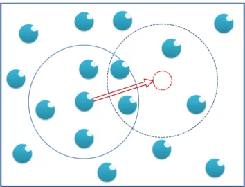
Figure 3.1: A particle displacement attempt in Metropolis Monte Carlo method.
reverts to its previous state is as likely as selecting any other state.
Anensemble(also statistical ensemble or thermodynamic ensemble) is an idealization consisting of a large number of mental copies of a system, considered all at once, each of which represents a possible state that the real system might be in [39]. One of the most common ensembles used in the literature is the
canonical ensemblewhere the number of particles (N), volume (V), and temperature (T) are fixed. However, the system energy (E) and pressure (P) are variables. This ensemble is also referred to as theNVTensemble.
Using Monte Carlo trials of different configurations, as per theBoltzmann’s Ergodic Hypothesis[10], this
method can give accurate physical information for many systems over a sufficient number of trials. The acceptance criteria in this case is typically given by first calculating the Boltzmann factor:
e(−β∆E), (3.1)
where∆E is the change in energy from the previous state to the tested state,β is given by(1/kBT),kB
is theBoltzmann constant, andT is the temperature of the system. The result of this equation is typically compared to a random number in the range[0,1). If the random number is higher than the Boltzmann factor, the move is accepted. This approach is known as the Boltzmann probability distribution [39].
25
3.1.2 Lennard-Jones Potential
The Lennard-Jones potential is a frequently used short-range interaction model to simulate interactions between a pair of particles [28]. The potential is given by:
ULJ = 4 σ r 12 −σ r 6 , (3.2)
whereis the depth of the potential well, σ is the collision diameter for interacting particles, andr is the distance between interacting particles. As can be observed, the mathematical succinctness of this formula en-courages its predominant use in the literature. From an implementation perspective, however, the simulation tends to be computationally intensive even for small systems. Specifically, the computation of interaction forces among molecules in a Lennard-Jones simulation which is given by the equation:
FLJ = 24 2 σ12 r13 − σ6 r7 . (3.3)
This portion of the simulation is responsible for nearly all of the execution time [70]. The complexity of computing particle interactions is typically reduced by maintaining the total system energy and computing only the change in energy of the system when a particle is displaced. Therefore, each displacement attempt takesO(N)time, whereN is the number of particles in the system.
The reader is referred to [39] for the proof of the validity of this method and further chemical details.
3.2
Structure of the Code
In order to gain a better understanding of my implementation, a high-level view of the serial algorithm is presented, see Algorithm 1. In this algorithm, an initial system energy is calculated, then a randomly chosen particle is moved to a random location. Finally, the acceptance rule is calculated as a function of the change in energy for that specific particle.
The CUDA architecture has some limitations that affect the system performance. For example, as the kernel cannot write directly to an output device, all system status and move results have to be copied back to the CPU for further processing and for output to files. Since the GPU and CPU do not share a common memory space, memory transfers are required to update the system status on the GPU if the CPU has changed
some shared variables and vice versa.
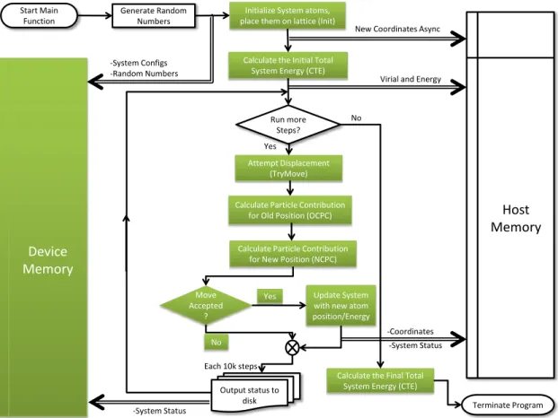
Developing a parallel GPU algorithm is largely domain driven. Our parallel algorithm has the same structure as the serial one due to the serial nature of the Monte Carlo algorithm. However, specific functions have been ported to the GPU. The flowchart in Figure 3.2 illustrates the main operations of the parallel implementation:
1. Generate a sequence of random numbers and move them asynchronously to the GPU along with system configuration parameters such as particle positions, current energy, current virial, number of particles in the system, etc.
2. Repeatedly perform trial move attempts within the main loop. For each trial pick a random particle to move a random distance in a random direction and calculate the difference in energy (∆E) for the selected particle in the old and new locations. This includes:
(a) Assign threads to particles
(b) Calculate partial energy sums from all threads (c) Calculate partial energy sums from all blocks (d) Assign the result to∆E
(e) Calculate the Boltzmann factor
3. Compare a random number to the resulting probability of acceptance calculated from the previous step 4. If the move is accepted, apply the changes to the system and adjust status
5. Periodically, output system status and particle positions to a data file 6. If there are more steps to execute, go to step 2
Figure 3.2 shows the hybrid CPU-GPU system, and illustrates data movement between the host and the device using double line arrows. Moreover, the data flow has been labeled to illustrate the specific data being transferred for that particular step. Eventually, the host has the main loop that the simulation executes, in
27
Algorithm 1Serial Canonical Ensemble Monte Carlo Algorithm
1: input: Number of particles and Volume
2: input: Temperature
3: input:,σ, rcut 4:
5: // Calculate initial energy of the system
6: fori = 1toN-2do
7: forj = i+1toNdo
8: total energy += calculate pairwise energy(i, j)
9: end for
10: end for
11: // Main Loop
12: for i = 1tostep numberdo
13: // Randomly select a particle to move
14: s = selected particle←rand()
15: Old particle loc←particle location(s)
16: // Randomly move to a new location
17: New particle loc←rand()
18: // Calculate the selected particle’s energy for the old and new locations
19: fork = 1toparticles, k! =sdo
20: old energy contrib += calculate pairwise energy(Old particle loc, k)
21: new energy contrib += calculate pairwise energy(New particle loc, k)
22: end for
23: deltaE = new energy contrib - old energy contrib
24: calculate acceptance rule()
25: if accepted then
26: total energy += deltaE
27: current config←new config
28: update system status()
29: else
30: //Leave current system state
31: end if
32: //Update the rate of accepted moves
33: // Solve if the system in equilibrium
34: // Periodically write system status to disk
Move Accepted
?
Attempt Displacement (TryMove)
Calculate Particle Contribution for Old Position (OCPC)
Start Main Function
Terminate Program
Calculate Particle Contribution for New Position (NCPC) Initialize System atoms, place them on lattice (Init)
Calculate the Initial Total System Energy (CTE)
Calculate the Final Total System Energy (CTE) Update System
with new atom position/Energy Run more Steps? Yes Yes No No Host Memory Device Memory
New Coordinates Async
Virial and Energy -System Configs -Random Numbers Generate Random Numbers Output status to disk -Coordinates -System Status Each 10k steps -System Status
Figure 3.2: Monte Carlo Simulation for the canonical Ensemble method flowchart. Kernel functions are in filled shapes.
29
addition to the I/O necessary to output system status to disk. The kernel functionTryMove() is responsible for handling the particle displacement attempt. The system energy and pressure are stored from the previous state and will be used to calculate the acceptance criteria for each displacement attempt. Moving this function to the device led to significantly better overall system performance, because the pairwise interactions can be calculated in parallel.
The Calculate Total Energy()function is another important function in this simulation. This function calculates the current system energy resulting from each interacting pair of particles, which requiresO(N2)
computations. Many optimizations have been applied to this function. The main focus was to balance the workload across the threads and hide the global memory latency. This function is executed only twice, at the beginning of the simulation to find the initial system energy and at the end of simulation for verification purposes.
3.3
Optimizing the canonical ensemble method for the GPU
In this section, we shall consider specific strategies implemented to optimize the canonical ensemble code. This list mentions a number of significant optimizations that have boosted the performance of this MC simulation. Since a parallel algorithm cannot be generalized to all problem domains, we have focused on the optimizations that enhanced the overall performance of this particular class of problems.
3.3.1 The block size effect
The number of threads per block is limited by resources that the device can allocate to each block. For devices of compute capability 1.x the maximum number of threads per block is 512 threads, and 1024 threads per block for devices of compute capability 2.x. One may think to load the GPU with the minimum number of threads per block so that less threads share resources per block to increase the performance. However, this is not the case. The main drawbacks to using smaller block sizes are the reduced sharing of data among threads and the limit on the maximum number of blocks that can run on an SM.
Threads in one block can share data through fast shared memory, blocks on the other hand can share data only through device global memory, which is much slower than shared memory. Another drawback for small block sizes is the need for synchronization mechanisms. While threads in the same block can synchronize
Table 3.1: Thread hierarchy and properties.
Coarse Size Associated Resources
Memory Scope Processing
Thread – registers, 1 core
local memory
Warp 32 threads registers, 1 SM
local memory
Block
512/1024 shared memory,
1 SM
threads for 1.x & L1, L2 cache
2.x compute cap.
Grid 65,536 per dim global, constant, device scope
64 on z-dim texture
execution through lightweight CUDA statements such as syncthreads(), threads in different blocks
need other techniques to accomplish synchronization such as the technique mentioned in section 3.3.7. In this study, several block sizes are examined and we have reported the performance measurements for each.
3.3.2 The use of pinned memory
Pinned memory enablesasynchronousmemory copies (allowing for overlap with both CPU and GPU
execution) as well as improving PCIe throughput. An example of using pinned memory in the NVT Monte Carlo simulation is the storage of pre-generated random numbers. Random numbers are needed for each step of the algorithm; we used the Mersenne Twister [77] random number generator on the CPU to produce a sequence of random numbers that are copied periodically and asynchronously from the CPU to the GPU. In addition, the system takes advantage of high throughput pinned memory when periodically transferring particle coordinates modified by the GPU to the CPU for checkpointing.
3.3.3 The use of different GPU memory types
Shared memory can be accessed by any thread in that particular block. Other blocks, on the other hand, have no access to this memory. Table 3.1 shows the GPU structures that can access shared memory. One of