Remote Sensing Data Assimilation in Dynamic Crop Models Using Particle Swarm Optimization

(1)

International Journal of

Geo-Information

Article

Remote Sensing Data Assimilation in Dynamic Crop

Models Using Particle Swarm Optimization

Matthias P. Wagner1,*, Thomas Slawig2 , Alireza Taravat1and Natascha Oppelt1 1 _{Earth Observation and Modelling, Dept. of Geography, Kiel University, 24118 Kiel, Germany;}

[email protected] (A.T.); [email protected] (N.O.) 2 _{Algorithmic Optimal Control—CO}

2Uptake of the Ocean, Dept. of Computer Science, Kiel University, 24118 Kiel, Germany; [email protected]

* Correspondence: [email protected]; Tel.:+49-176-5788-6714

Received: 14 December 2019; Accepted: 7 February 2020; Published: 10 February 2020 Abstract: A growing world population, increasing prosperity in emerging countries, and shifts in energy and food demands necessitate a continuous increase in global agricultural production. Simultaneously, risks of extreme weather events and a slowing productivity growth in recent years has caused concerns about meeting the demands in the future. Crop monitoring and timely yield predictions are an important tool to mitigate risk and ensure food security. A common approach is to combine the temporal simulation of dynamic crop models with a geospatial component by assimilating remote sensing data. To ensure reliable assimilation, handling of uncertainties in both models and the assimilated input data is crucial. Here, we present a new approach for data assimilation using particle swarm optimization (PSO) in combination with statistical distance metrics that allow for flexible handling of model and input uncertainties. We explored the potential of the newly proposed method in a case study by assimilating canopy cover (CC) information, obtained from Sentinel-2 data, into the AquaCrop-OS model to improve winter wheat yield estimation on the pixel- and field-level and compared the performance with two other methods (simple updating and extended Kalman filter). Our results indicate that the performance of the new method is superior to simple updating and similar or better than the extended Kalman filter updating. Furthermore, it was particularly successful in reducing bias in yield estimation.

Keywords: particle swarm optimization (PSO); AquaCrop-OS; data assimilation; uncertainty quantification; crop yield estimation; model updating; canopy cover (CC)

1. Introduction

After decades of continuously rising yields, recent years have seen a slowing down in agricultural productivity growth in Europe. Furthermore, decreasing global production may be expected under certain climate scenarios [1,2]. Simultaneously, a growing world population, rising income per capita, and increasing demand for energy are expected to drive demand for agricultural products [3,4]. Combined with increasing risks of extreme weather events, these factors emphasize the need for timely and accurate crop production monitoring. A common approach is the use of dynamic biophysical crop models that simulate the soil–plant–atmosphere interface [5]. These models can simulate environmental interactions and field management, but have a limited capacity to represent geospatial information on larger scales.

To address this drawback, remote sensing imagery and crop models can be merged. Remote sensing can introduce high-resolution spatial information about plant development and health into the modeling process. The increasing availability of free satellite data helps to reduce costs, especially when replacing traditional field measurements or airborne campaigns. The abundance of data from the

(2)

Landsat archive and the Copernicus program by the European Space Agency (ESA) further fosters the integration of satellite data into crop models [6].

Following the early work by Delécolle et al., crop model data assimilation techniques may be categorized into three broad groups: forcing, re-calibration, and updating [7]. Forcing refers to the replacement of simulated values with measured data. This method is very efficient and easy to implement, but has several drawbacks. First, it requires measurements for each simulation step (e.g., daily observations), which are often unavailable or need to be interpolated. When integrating optical remote sensing data, in particular, frequent cloud cover can drastically reduce the number of available observations, even with shorter revisit times in constellations such as Sentinel-2. Second, forcing effectively breaks up the simulation loop because it replaces intermediate results with external inputs [8]. Third, it does not consider measurement uncertainties and therefore directly transfers errors to the model. Due to these drawbacks, a few recent studies have considered forcing.

A frequently applied technique is re-calibration, sometimes separated into re-initialization and re-parametrization. Here, the initial values and parameters of the crop model are iteratively changed by minimizing a cost function measuring the distance between the simulated state variables and observed ones [7,9]. Re-calibration therefore obtains a new set of parameters or initial values, thus allowing a simulation that resembles better observations. Although this method often improves model-based yield predictions, it has two flaws. First, re-calibration settings may be unrealistic or may represent an unreliable parameter setup [9]. Second, re-calibration can be computationally demanding because it requires multiple re-runs of the model, hampering larger scale applications.

Updating performs the assimilation during the simulation, only interfering when an observation is available. It therefore performs well even with few and infrequent observations and reduces processing time when compared to re-calibration. Furthermore, updating allows uncertainties in both the simulation and the data assimilated to be addressed [10]. However, it requires modifications in the model itself (i.e., the source code) and not all models allow such interference. The most commonly used updating techniques are the (extended) Kalman filter, particle filter, and the ensemble Kalman filter [11–14].

Following the definition by Kennedy and O’Hagan, model uncertainties may be classified into parameter, parametric, model inadequacy, residual variability, observation, and code uncertainties [15]. In the context of biophysical modeling, the most relevant sources of uncertainties are parameter uncertainty (errors related to suboptimal parameter settings), parametric or input uncertainty (errors in the input data driving the simulation, e.g., daily weather measurements), code uncertainty (approximations and inaccuracies in model implementation), and model inadequacy (e.g., model bias). Uncertainties related to implementations and inadequacies are usually addressed during model development and subsequent calibration and sensitivity studies [16–19]. Parameter and input uncertainties, however, are highly application- and context-dependent and need to be assessed individually.

Most updating approaches are robust and fast, but often lack a detailed representation of such uncertainties. The Kalman filter, for example, approximates uncertainties in the model and the measurement by a simple scalar (e.g., the standard deviation in repeated measurements) or a covariance matrix in the case that multiple variables are updated [20]. This approach does not allow for a detailed handling of different uncertainty sources. Techniques such as the above-mentioned ensemble Kalman or particle filter, may account for uncertainty in parameters and model states stochastically.

Both re-calibration and updating require the solution of an optimization problem, which is usually non-linear. For such kinds of problems, several numerical algorithms can be applied. In our updating technique, we employed particle swarm optimization (PSO) due to its reliable global optimization capacities and flexibility in inputs and objective functions (see Section2.2.3). PSO has seen various applications in remote sensing, frequently in image segmentation and classification [21–23], but also in agricultural applications. Guo et al., for example, used the algorithm to couple the PROSAIL canopy reflectance model with the WheatGrow crop model based on vegetation indices [24]. Others have

(3)

ISPRS Int. J. Geo-Inf.2020,9, 105 3 of 24

used it in combination with multiple classifiers and algorithms for crop classification [25]. The most frequent application, however, is the (re-)calibration of crop models such as the WOrld FOod STudies model (WOFOST) [26], the Simple Algorithm for Yield Estimate (SAFY) [27], the Decision Support System for Agrotechnology Transfer (DSSAT) [28,29], or AquaCrop [30,31].

The main objective of this study was therefore to ensure increased flexibility of uncertainty handling. The new technique proposed allows the user to include different uncertainties in the process with minimal limitations on their type and definition. The technique should also be largely independent and self-calibrating to enable direct application with minimal prior adjustments, thus allowing fast assimilation of remote sensing observations.

Although many studies exist that combine remote sensing inputs with dynamic crop models, a direct comparison is difficult to draw. The diverse nature of approaches involving different sensors, input variables, crop types, crop models, calibration settings, application scales (field to national or even continental and global) and varying amounts of prior knowledge (e.g., detailed study plots with regular measurements), aggravate a direct comparison. To demonstrate the potential of the new method, we therefore decided to apply multiple updating schemes to the same datasets with the same model and calibration settings. We compared the results of the new approach to a simple updating scheme (replacing values in the model simulation directly) as well as an extended Kalman filter (EKF). As a case study, we assimilated Sentinel-2 canopy cover (CC) data into the AquaCrop-OS model v5.0a to improve the winter wheat yield estimation.

The rest of the paper consists of five parts. Section2describes the study area and data used and introduces the methodology. We provide some methodological background first, followed by a description of the updating technique. In Section3, we describe results and discuss them in Section4. Finally, Section5will give a short conclusion and outlook.

2. Materials and Methods 2.1. Datasets

2.1.1. Study Area

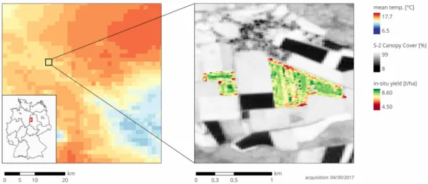
Our study area is located in central Germany near the border of the states of Niedersachsen and Sachsen-Anhalt (see Figure1). The climate is temperate/oceanic with warm summers and wet winters (Cfb in Koeppen-Geiger climate classification) [32]. The region is relatively warm and dry with an average temperature of 8.2◦C and an annual precipitation of 538 mm in the climate reference period 1960–1990 [33]. Our weather data of the years 2016 and 2017 revealed both years to be rather warm (9.8 and 10.8◦C), while precipitation was low in 2016 (436 mm) and high in 2017 (679 mm) compared to the long-term average. Soils in the region are typically stagnosols and brown earths originating from sandy and loamy glacial debris. Further, clayey soils from skeletal loam, sandy Loess over limestone, rendzinas, and some podzols also occur [34].

(4)

Sentinel-2 Toolbox (S2TBX, version 6.0.4) to generate canopy cover (CC) maps from all scenes (see Figure 1). The processor employs artificial neural networks trained on a large dataset of radiative transfer simulations of canopy and leaf properties [36]. The documentation of the SNAP Biophysical Processor provides some theoretical performance indicators. The authors claim a low root mean square error (RMSE) of 0.04 for CC predictions on their validation dataset [36]. During pre-processing, we further performed a multi-threshold cloud and cloud shadow detection for each of our test fields to discard any potentially contaminated observations. The resulting number of observations ranged between three and 12 per growing season, depending on location.

2.1.4. Yield Data

Field data were obtained via GPS-based yield measurements on combine harvesters during harvest of 30 fields in 2016 and 32 fields in 2017. We removed outliers outside +/− 2.58 standard deviations (99% threshold in a standard normal distribution), particularly false zero measurements that frequently occurred at the start and end of the harvest procedure. We then aggregated the remaining points to 10 x 10 m² yield maps matching Sentinel-2 observations (see Figure 1). The resulting mean yields of all fields were in good agreement with the reported department-level yield statistics [37–39]. The observed yield on the pixel-level ranged from 2.38 to 9.60 t/ha, and the mean field yields ranged from 3.90 to 7.63 t/ha. No information on measurement accuracy was provided.

For further analysis, we generated a pixel- and a field-level dataset. We split both randomly into 60% calibration (32 field observations, 23,375 pixel observations) and 40% validation (20 field observations, 15,584 pixel observations) data.

Figure 1. Map of study area and example of rasterized weather datasets in the form of mean air temperature (left). Example of yield data and canopy cover maps (right).

2.2. Methodological Background

2.2.1. AquaCrop-OS Description

AquaCrop is a dynamic crop model developed by the Food and Agriculture Organization of the United Nations (FAO). It simulates the yield response of herbaceous crops on a homogeneous field, considering water response and various stress effects [40–42]. Inputs for daily simulation are the maximum and minimum temperature data, precipitation sum, and potential evapotranspiration [43]. The simulation is considerably simplified compared to complex model suites such as the Decision Support System for Agrotechnology Transfer (DSSAT) [44,45], focusing on a global model applicability with a potentially limited range of available data.

The central part of the model is a crop productivity function that relates biomass accumulation to water productivity and evapotranspiration to obtain the total cumulative biomass:

Figure 1. Map of study area and example of rasterized weather datasets in the form of mean air temperature (left). Example of yield data and canopy cover maps (right).

2.1.2. Weather Data

The German Weather Service (DWD) delivered daily weather data for the nearby weather station “Ummendorf” (11.18◦E, 52.16◦N) as well as 1×_{1 km}2_{rasterized weather datasets for the whole}

of Germany (see Figure 1). Weather data include daily minimum and maximum temperatures,

precipitation sums, and reference evapotranspiration based on the Penman–Monteith equation [35]. The raster datasets were used as input to the model, introducing a limited amount of spatial dynamics. 2.1.3. Canopy Cover Data

Our database consisted of atmospherically corrected Sentinel-2 Level-2A scenes between August 2015 and November 2017. We only considered scenes with generally low to moderate cloud cover (up to 50%). The dataset comprised of 116 scenes, covering the full winter wheat growing seasons for both harvest periods of 2016 and 2017. We used the biophysical processor implemented in the ESA Sentinel-2 Toolbox (S2TBX, version 6.0.4) to generate canopy cover (CC) maps from all scenes (see Figure1). The processor employs artificial neural networks trained on a large dataset of radiative transfer simulations of canopy and leaf properties [36]. The documentation of the SNAP Biophysical Processor provides some theoretical performance indicators. The authors claim a low root mean square error (RMSE) of 0.04 for CC predictions on their validation dataset [36]. During pre-processing, we further performed a multi-threshold cloud and cloud shadow detection for each of our test fields to discard any potentially contaminated observations. The resulting number of observations ranged between three and 12 per growing season, depending on location.

2.1.4. Yield Data

Field data were obtained via GPS-based yield measurements on combine harvesters during harvest of 30 fields in 2016 and 32 fields in 2017. We removed outliers outside+/−_{2.58 standard}

deviations (99% threshold in a standard normal distribution), particularly false zero measurements that frequently occurred at the start and end of the harvest procedure. We then aggregated the remaining points to 10 x 10 m2yield maps matching Sentinel-2 observations (see Figure1). The resulting mean yields of all fields were in good agreement with the reported department-level yield statistics [37–39]. The observed yield on the pixel-level ranged from 2.38 to 9.60 t/ha, and the mean field yields ranged from 3.90 to 7.63 t/ha. No information on measurement accuracy was provided.

For further analysis, we generated a pixel- and a field-level dataset. We split both randomly into 60% calibration (32 field observations, 23,375 pixel observations) and 40% validation (20 field observations, 15,584 pixel observations) data.

(5)

2.2. Methodological Background

2.2.1. AquaCrop-OS Description

AquaCrop is a dynamic crop model developed by the Food and Agriculture Organization of the United Nations (FAO). It simulates the yield response of herbaceous crops on a homogeneous field, considering water response and various stress effects [40–42]. Inputs for daily simulation are the maximum and minimum temperature data, precipitation sum, and potential evapotranspiration [43]. The simulation is considerably simplified compared to complex model suites such as the Decision Support System for Agrotechnology Transfer (DSSAT) [44,45], focusing on a global model applicability with a potentially limited range of available data.

The central part of the model is a crop productivity function that relates biomass accumulation to water productivity and evapotranspiration to obtain the total cumulative biomass:

BT = Ksb·WP ∗_· T X t=0 _Trt ETot (1)

whereBTis the total accumulated biomass fromt=0 days tot=T;Ksbis an air temperature stress

coefficient;WP∗

is the water productivity normalized to annual mean CO2concentration;Trtis daily

crop transpiration; andETotis daily potential evapotranspiration (both in mm).

AquaCrop represents the heat, drought, and cold stress effects via stress coefficients that can influence canopy development, stomatal conductance, canopy senescence, or harvest index development. The stress coefficients change with the level of stress following a convex to concave response curve [41,46]:

Ks = 1− e

S_relf_shape₋

1

eS_rel−₁ (2)

whereKsdescribes the stress response function;Srelis the relative stress level (≤_{1); and} _fshape_{is a shape}

factor defining the curvature of the function.

The main state variable in the model is canopy cover (CC; sometimes referred to as Fraction of Vegetation Cover, FVC or FCOVER) that directly influencesTrtin Equation (1) via a crop transpiration coefficient:

KC_Tr = CC∗KC_Tr_,_x (3)

Tr = KswKCTr ETo (4)

whereCC∗is the current canopy cover (adjusted for micro-adjective effects);KC_Tr_,_x is the maximum crop transpiration coefficient for well-watered soil and a complete canopy;Kswrepresents a soil water stress coefficient; andKCTris the current crop transpiration coefficient obtained. Therefore, CC is an important variable in biomass accumulation in Equation (1), and consequentially, yield as determined via a harvest index (i.e., percentage of biomass at crop maturity).

CC development over the growing season is determined mostly empirically. After crop emergence, CC first increases exponentially up to 50% of the maximum. A slowing growth follows until the maximum is reached. The value of CC stays constant until an exponential decay sets in at the beginning of senescence [46]. This process is summarized in the following equations:

Canopy expansion:CC= CCoet CGC f or CC ≤ CCx

2 (5) CC= CCx−_0.25 (CCx) 2 CC0 e −_{t CGC} f or CC > CCx 2 (6) Canopy senescence:CC= CCx 1−_0.05 eCDCCCx −₁ f or CC ≤ CCx 2 (7)

(6)

whereCCis the new canopy cover; CCx is the maximum possible canopy cover;CCois the initial canopy cover at the start of growth; andCGCandCDCare canopy growth and decline coefficients, respectively. Dry yield is obtained by applying a harvest index (percentage) to the biomass value at maturity.

We used the open source version of the model called AquaCrop-OS, allowing us to make the necessary source code changes for the updating procedures described in Section2.3[47].

2.2.2. AquaCrop-OS Calibration

Due to the lack of information on winter wheat varieties on our test fields or regular in situ sampling, our prior knowledge for calibration was limited. We therefore relied on an empirical calibration of model parameters. This also made the simulation more general and independent of specific field conditions.

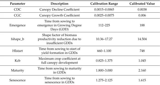
AquaCrop-OS offers a large number of crop parameters, separated into conservative ones that have previously been proven accurate in many different environments and user-specific ones [43]. The former were ignored for the most part in our calibration, except for the Canopy Growth and Decline Coefficients (CGC and CDC, see Table1) due to their particular relevance in this context. We did not consider irrigation management because agriculture in our study area is exclusively rain-fed. Similarly, we assumed that field management follows a “best practice” due to high technological standards and a long tradition of industrialized agriculture in our study area.

Table 1.Calibration ranges and obtained calibrated crop parameters in AquaCrop-OS.

Parameter Description Calibration Range Calibrated Value

CDC Canopy Decline Coefficient 0.0015–0.0065 0.0038 CGC Canopy Growth Coefficient 0.0025–0.0075 0.006 Emergence

Time from sowing to emergence in Growing Degree

Days (GDD)

112–225 188

fshape_b

Shape factor of biomass productivity reduction due to

insufficient GDDs

10.36–17.27 14.504

HIstart Time from sowing to start of

yield formation in GDDs 660–1.100 748

Kcb Maximum crop coefficient at

full canopy development 0.825–1.375 1.045 Maturity Time from sowing to maturity

in GDDs 1.800–3.000 2.160

Senescence Time from sowing to

senescence in GDDs 1.275–2.125 1.615

We performed a sensitivity analysis based on iterative changes to individual parameters and observed the influence on predicted yield. It revealed the parameters listed in Table1to be those most relevant for winter wheat yield prediction in our study area. We calibrated the model by altering parameters iteratively and minimizing the RMSE of yield. The calibration process improved the RMSE from 2.305 t/ha to 1.324 t/ha on field-level and from 2.264 t/ha to 1.521 t/ha on the pixel-level validation datasets. The optimal parameter settings for the pixel- and field-level were quite similar, so we decided to use the same calibration set on both scales. Table1provides a list of calibration settings.

2.2.3. Particle Swarm Optimization

Particle swarm optimization is a metaheuristic global optimization algorithm based on swarm intelligence principles of complex intelligent behavior emerging from primitive individual agents.

(7)

As such, it is part of the larger family of evolutionary computing [48,49]. Kennedy and Eberhart originally designed the algorithm following previous efforts by Reynolds in simulating realistic movements of bird flocks [50,51].

The particle swarm is a group (“swarm”) of candidate solutions (“particles”) moving in the multidimensional search space over time (i.e., iteration steps). Each particle is initiated as a random vector with a random initial velocity vector representing its movement in the search space. This velocity is updated at each iteration based on certain rules and the new particle fitness is obtained. In the original version, the process is only influenced by the best previous solution of the particle (previous best, pbest) and the best solution obtained in its neighborhood (neighborhood best, nbest) [48,49]. This neighborhood is described by the topology representing connections between the particles in the swarm. There are many different topologies used in the literature including local best, global best, and von Neumann topologies, but also dynamic topologies changing throughout the process based on time, Euclidian distance, and fitness–distance ratios, among others [52,53]. For a more detailed discussion, readers may refer to the paper by Poli et al. [54].

The following equations describe the central velocity and position update (all multiplications are element-wise): * vi(t) = *vi(t−1) + ϕ11 * p_i− *_x_i_(t−₁₎₊ ϕ₂₂*_p n− * xi(t−1) (8) * xi(t) = * xi(t−1) + * vi(t) (9)

where*vi(t)is the new (updated) velocity vector of particleiat time steptand *

vi(t−1)is its previous

velocity vector. The previous and new positions are given by*xi(t−1)and*xi(t), respectively. The

previous best solution is represented by*p_iand the neighborhood best solution by*p_n. The termsϕ1

andϕ2refer to pbest and nbest coefficients, respectively, and1,2are random vectors [48]. One can

interpret pbest and nbest coefficients as the tendency of particles to move independently or “toward the swarm”. The two elements are therefore closely related to exploration and exploitation.

Its metaheuristic approach distinguishes PSO from gradient-based optimization techniques. PSO does not use exact or approximated derivative information. It therefore does not need continuous or differentiable objective functions or any prior knowledge about the cost function [55]. This makes it very flexible in handling different types of inputs and even combinations of continuous and discrete functions. PSO is also considered to be reliable in finding global optima, even in highly heterogeneous, complex solution spaces as simulated by test functions like the Ackley or Hölder table functions [48,56]. Moreover, PSO scales very well with high-dimensional inputs as the number of function evaluations is determined by the swarm size, not the number of input variables.

However, PSO is not a deterministic algorithm, but includes stochastic elements. The process is therefore not entirely predictable, even identical starting conditions may lead to different iteration steps and even to different solutions due to the random component of the process [54]. As a result, it is up to the user to determine application-specific parameters (such as swarm size, coefficients, topology, etc.) that ensure a reliable and fast convergence. Furthermore, unlike gradient descent-related algorithms that reach a local minimum under certain assumptions, the convergence in PSO methods is only valid in a stochastic setting.

To ensure fast and reliable optimization results, we compared a number of different PSO variants and settings. This included different swarm sizes, inertia weights, cognitive and social coefficients, static and dynamic topologies (local best, global best, dynamic nearest neighbor, dynamic fitness–distance ratio, among others) as well as different distributions for random vector sampling (uniform, normal, Lévy).

We observed that Clerc’s constriction coefficients [57] were superior to inertia weights or velocity bounds alone. We therefore usedϕ1=ϕ2=2.05, and the constriction coefficientχcalculated according

to [57]. We further observed that, although not necessarily required when using inertia weights or constriction coefficients, limitingvmaxto the dynamic range of the input was advantageous in some

(8)

cases, as suggested in [58]. The von Neumann and dynamic nearest neighbor topologies showed quite similar performances with the former being chosen due to higher computational efficiency. Different random distributions showed no significant impact in this context. The swarm size was set to 20, a common value in the literature. Larger numbers of particles were unable to improve convergence significantly, but logically increased the number of function evaluations, slowing down the process. Table2presents the fastest and most reliable setup we obtained. In our applications, this implementation usually converged very quickly to the optimum within 10–15 iterations.

Table 2.Settings used for particle swarm optimization algorithm.

Parameter Value

swarm size (n) 20

pbest coefficient (ϕ1) 2.05 nbest coefficient (ϕ2) 2.05 maximum velocity (vmax) dynamic range constriction coefficient (χ) ~0.72984

topology von Neumann (4 neighbors) random distribution uniform

2.2.4. Uncertainty Quantification

We considered multiple sources of uncertainties, both in the model and the remote sensing data. These need to be quantified before they can be included in the updating procedure. We are unable to account for potential weather measurement errors or instrument-related issues. Still, we are able to quantify the reaction of AquaCrop-OS canopy cover simulations to perturbations in weather inputs and parameter settings.

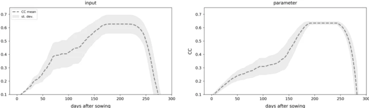
We achieved this via Monte Carlo simulations. First, we estimated input-related uncertainty by randomly perturbing a 10-year mean weather time series with Gaussian random noise. The magnitude of the noise was determined by the daily variance observed in the same 10-year period. We obtained 10,000 CC time series from AquaCrop-OS simulations on these randomized weather datasets. Second, we assessed parameter uncertainties accordingly by randomly sampling parameter settings from a normal distribution around the calibrated values in Table1with a standard deviation of 1/10 of the calibration range. This ensured a sufficient variation within a realistic range around the calibrated settings. We performed 10,000 Monte Carlo simulations randomizing all parameters listed in Table1. Both model-related uncertainties are illustrated in Figure2. Third, we estimated uncertainties in the remote sensing data. Here, the procedures on field- and pixel-level are different. On the field level, we used a set of all CC pixel values in a given field at the observation date; on the pixel-level, we used only values in the 3×_{3 pixel neighborhood (see Figure}₃_).

ISPRS Int. J. Geo-Inf. 2019, 8, x FOR PEER REVIEW 8 of 24

constriction coefficient (𝜒) ~0.72984

topology von Neumann (4 neighbors)

random distribution uniform

2.2.4. Uncertainty Quantification

We considered multiple sources of uncertainties, both in the model and the remote sensing data. These need to be quantified before they can be included in the updating procedure. We are unable to account for potential weather measurement errors or instrument-related issues. Still, we are able to quantify the reaction of AquaCrop-OS canopy cover simulations to perturbations in weather inputs and parameter settings.

We achieved this via Monte Carlo simulations. First, we estimated input-related uncertainty by randomly perturbing a 10-year mean weather time series with Gaussian random noise. The magnitude of the noise was determined by the daily variance observed in the same 10-year period. We obtained 10,000 CC time series from AquaCrop-OS simulations on these randomized weather datasets. Second, we assessed parameter uncertainties accordingly by randomly sampling parameter settings from a normal distribution around the calibrated values in Table 1 with a standard deviation of 1/10 of the calibration range. This ensured a sufficient variation within a realistic range around the calibrated settings. We performed 10,000 Monte Carlo simulations randomizing all parameters listed in Table 1. Both model-related uncertainties are illustrated in Figure 2. Third, we estimated uncertainties in the remote sensing data. Here, the procedures on field- and pixel-level are different. On the field level, we used a set of all CC pixel values in a given field at the observation date; on the pixel-level, we used only values in the 3 × 3 pixel neighborhood (see Figure 3).

Using these datasets, we created probability density functions (PDF) representing the probability of all possible CC values (between 0 and 1) of each uncertainty source. We employed kernel density estimation with a symmetric Gaussian kernel. Tests showed that a narrow bandwidth of 0.02 yielded the best results. Finally, we represented the uncertainty in the current simulation by a Gaussian distribution around the currently simulated CC value using a bandwidth of 0.2.

Figure 2. Visualization of observed uncertainties throughout the growing season. Uncertainty from Monte Carlo simulations weather inputs (left) and perturbing parameters (right).

Figure 2.Visualization of observed uncertainties throughout the growing season. Uncertainty from Monte Carlo simulations weather inputs (left) and perturbing parameters (right).

(9)

ISPRS Int. J. Geo-Inf.2020,9, 105 9 of 24 ISPRS Int. J. Geo-Inf. 2019, 8, x FOR PEER REVIEW 9 of 24

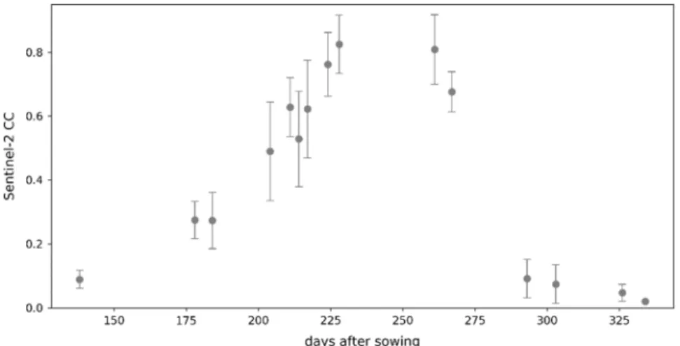
Figure 3. Example of uncertainties in Sentinel-2 CC values in a field. Dots refer to the mean of all CC observations (i.e., pixels) in the field, error bars indicate standard deviations.

2.3. Updating Methodology 2.3.1. Simple Updating

The simple updating scheme we employed replaced simulated CC values directly with remote sensing observations without any additional processing and with no consideration of uncertainties. As a result, the simulated CC values remained unconsidered and errors in the remote sensing data were directly transferred to the model.

2.3.2. Extended Kalman Filter Updating

Since its first description in [11], the Kalman filter has become one of the most common data assimilation techniques [20]. It iteratively updates an estimated value by incorporating information from incoming measured values, taking into account the uncertainty associated with both the measurement and the estimated value. The Kalman filter assumes a linear model. Its extension to non-linear models is the EKF. Here, a linearization of the original non-linear model function is used to update the uncertainty (i.e., the covariance matrix) of the estimate of the model state [14,59].

In our case, we have a non-linear model, but we assimilated the scalar state variable CC directly. Thus, no additional observation is present. Both facts simplify the EKF procedure and make the updating computationally very efficient. Assuming we have the estimates of the state variable 𝑥 and its uncertainty 𝑃 at time step instant 𝑡 . We now obtain a new observation value 𝑦 at the next time instant 𝑡 . Then, the EKF performs a predictor step for the model state

𝑥 = 𝑓(𝑥 ) (10) using the original non-linear model. Additionally, the uncertainty is predicted as:

𝑃 = 𝐹 𝑃 𝐹 (11) Here, we assume that the model has no error and uses an approximation 𝐹 𝑓′(𝑥 ) for the derivative of the model function. In our case, this derivative is also a scalar. Now, the Kalman gain is computed as:

𝐺 = 𝑃

𝑃 + 𝑅 (12) where 𝑅 is the uncertainty in the measurement 𝑦 . Now, the correction step computes new estimates of the state and its uncertainty as:

Figure 3.Example of uncertainties in Sentinel-2 CC values in a field. Dots refer to the mean of all CC observations (i.e., pixels) in the field, error bars indicate standard deviations.

Using these datasets, we created probability density functions (PDF) representing the probability of all possible CC values (between 0 and 1) of each uncertainty source. We employed kernel density estimation with a symmetric Gaussian kernel. Tests showed that a narrow bandwidth of 0.02 yielded the best results. Finally, we represented the uncertainty in the current simulation by a Gaussian distribution around the currently simulated CC value using a bandwidth of 0.2.

2.3. Updating Methodology

2.3.1. Simple Updating

The simple updating scheme we employed replaced simulated CC values directly with remote sensing observations without any additional processing and with no consideration of uncertainties. As a result, the simulated CC values remained unconsidered and errors in the remote sensing data were directly transferred to the model.

2.3.2. Extended Kalman Filter Updating

Since its first description in [11], the Kalman filter has become one of the most common data assimilation techniques [20]. It iteratively updates an estimated value by incorporating information from incoming measured values, taking into account the uncertainty associated with both the measurement and the estimated value. The Kalman filter assumes a linear model. Its extension to non-linear models is the EKF. Here, a linearization of the original non-linear model function is used to update the uncertainty (i.e., the covariance matrix) of the estimate of the model state [14,59].

In our case, we have a non-linear model, but we assimilated the scalar state variable CC directly. Thus, no additional observation is present. Both facts simplify the EKF procedure and make the updating computationally very efficient. Assuming we have the estimates of the state variablexkand

its uncertaintyPkat time step instanttk. We now obtain a new observation valueyk+1at the next time

instanttk+1. Then, the EKF performs a predictor step for the model state

ˆ

xk+1= f(xk) (10)

using the original non-linear model. Additionally, the uncertainty is predicted as: ˆ

(10)

Here, we assume that the model has no error and uses an approximationFk ≈ f0(xk)for the

derivative of the model function. In our case, this derivative is also a scalar. Now, the Kalman gain is computed as: Gk+1= ˆ Pk+1 ˆ Pk+1+ Rk+1 (12) whereRk+1is the uncertainty in the measurement yk+1. Now, the correction step computes new

estimates of the state and its uncertainty as:

xk+1= xkˆ+1+ Gk+1(yk+1− xkˆ +1) (13)

Pk+1= (1−Gk+1)Pkˆ +1 (14)

We computed the derivative approximation needed in Equation (11) by a finite difference formula:

Fk= f(xk)− _f_(xk−₁) xk−xk−₁ = xkˆ +1−xkˆ xk−xk−₁ (15) This approximation uses only already computed quantities. In the first assimilation step (k=0), a modification is needed to replace the valuexk−₁and f(x_k−₁).

As mentioned previously, after accounting for clouds and cloud shadows, the remaining observations were not too frequent. In case of frequent observations, the updated uncertainty can be propagated continuously throughout the whole EKF process. In our case, however, we often encountered large time gaps in between observations. This implies that the assimilation cannot take place in every time step of the model. Thus, the function f in Equation (10) represents not just one model step, but rather summarizes a concatenation of model steps between subsequent time instants

tkandtk+1where measurements are available. As a consequence, the derivative approximation in

Equation (15) is an average of the derivative of the model in the interval [tk,tk+1]. As indicated in

Section2.2.1, AquaCrop-OS varies significantly in its simulation procedures depending on growth stages and environmental influences. Thus, this kind of averaging of the derivative seems to be reasonable. As noted above, the derivative for the first assimilation step has to be approximated in a slightly different way. Here, we used a state at a time instant in the interval [t=0,t1] instead ofxk−₁.

The uncertainty in the state is initially assumed to be 0.2. The uncertainty in the measured values was estimated as the standard deviation of all CC values at the observed location and time (i.e., all pixels of a field on the field-level and pixels in the 3×_{3 neighborhood on the pixel-level).}

2.3.3. New Updating Scheme

Figure4demonstrates the main processing steps for our new method. Preparation of CC data (green), weather data (blue), and yield maps (yellow) were discussed in Section2.1and uncertainty quantification (dark blue) was covered in Section2.2.4. In this section and the next, we will explain the details of the actual updating process and accuracy assessment (grey).

The fundamental idea behind our approach is to balance all uncertainties (relating to the model and the CC observations) to obtain the updated value. To do so, we represented all uncertainties as PDFs (see Section2.2.4). We then obtained a hypothetical optimal Gaussian distribution, as described by a meanµand a standard deviationσ, that balances all uncertainties in terms of statistical distance (see Figure5). In other words, we assumed that the mean of a distribution minimizing statistical distances to all PDFs will provide us with a better estimate given the available information. We employed PSO to search for the mean and standard deviation of this optimal Gaussian distribution.

(11)

𝑥 = 𝑥 + 𝐺 (𝑦 − 𝑥 ) (13) 𝑃 = (1 − 𝐺 ) 𝑃 (14) We computed the derivative approximation needed in Equation (11) by a finite difference formula:

𝐹 = 𝑓(𝑥 ) − 𝑓(𝑥 ) 𝑥 − 𝑥 =

𝑥 − 𝑥

𝑥 − 𝑥 (15) This approximation uses only already computed quantities. In the first assimilation step (𝑘 = 0), a modification is needed to replace the value 𝑥 and 𝑓(𝑥 ).

As mentioned previously, after accounting for clouds and cloud shadows, the remaining observations were not too frequent. In case of frequent observations, the updated uncertainty can be propagated continuously throughout the whole EKF process. In our case, however, we often encountered large time gaps in between observations. This implies that the assimilation cannot take place in every time step of the model. Thus, the function 𝑓 in Equation (10) represents not just one model step, but rather summarizes a concatenation of model steps between subsequent time instants 𝑡 and 𝑡 where measurements are available. As a consequence, the derivative approximation in Equation (15) is an average of the derivative of the model in the interval [𝑡 , 𝑡 ]. As indicated in Section 2.2.1, AquaCrop-OS varies significantly in its simulation procedures depending on growth stages and environmental influences. Thus, this kind of averaging of the derivative seems to be reasonable. As noted above, the derivative for the first assimilation step has to be approximated in a slightly different way. Here, we used a state at a time instant in the interval [𝑡 = 0, 𝑡 ] instead of 𝑥 . The uncertainty in the state is initially assumed to be 0.2. The uncertainty in the measured values was estimated as the standard deviation of all CC values at the observed location and time (i.e., all pixels of a field on the field-level and pixels in the 3 × 3 neighborhood on the pixel-level).

2.3.3. New Updating Scheme

Figure 4 demonstrates the main processing steps for our new method. Preparation of CC data (green), weather data (blue), and yield maps (yellow) were discussed in Section 2.1 and uncertainty quantification (dark blue) was covered in Section 2.2.4. In this section and the next, we will explain the details of the actual updating process and accuracy assessment (grey).

Figure 4. Flowchart of pre-processing steps and the new updating algorithm. Colors refer to different aspects: Sentinel-2 CC data (green), weather input data (blue), yield data preparation (yellow), uncertainty quantification (dark blue), and the actual simulation and updating process (grey).

Figure 4.Flowchart of pre-processing steps and the new updating algorithm. Colors refer to different aspects: Sentinel-2 CC data (green), weather input data (blue), yield data preparation (yellow), uncertainty quantification (dark blue), and the actual simulation and updating process (grey).

ISPRS Int. J. Geo-Inf. 2019, 8, x FOR PEER REVIEW 11 of 24 The fundamental idea behind our approach is to balance all uncertainties (relating to the model and the CC observations) to obtain the updated value. To do so, we represented all uncertainties as PDFs (see Section 2.2.4). We then obtained a hypothetical optimal Gaussian distribution, as described by a mean 𝜇 and a standard deviation 𝜎, that balances all uncertainties in terms of statistical distance (see Figure 5). In other words, we assumed that the mean of a distribution minimizing statistical distances to all PDFs will provide us with a better estimate given the available information. We employed PSO to search for the mean and standard deviation of this optimal Gaussian distribution.

Figure 5. Idealized representation of optimal Gaussian distribution (solid dark grey line) and summed uncertainty probability density functions (solid light grey lines). Maximum likelihood estimators (MLE) of the uncertainty probability density functions indicated by vertical dotted lines, updated CC value (i.e., location of optimal Gaussian distribution) indicated by vertical dashed line. This example represents a common case in our tests with model-related uncertainties and remote sesnsing observations indicating different value ranges for optimal CC (based on [60]).

The central element of this technique is the representation of distance or similarity between probability distributions or their respective PDFs. There are a number of statistical distance and divergence metrics proposed in the literature. Some of the most common ones are the Hellinger distance, the Kullback–Leibler divergence, and Bhattacharyya distance [61–63].

When comparing calculations measuring the statistical distance of the optimal Gaussian distribution to a set of uncertainty PDFs, the different metrics behaved similarly. Figure 6 demonstrates this with example cases where three PDFs at different locations and with different standard deviations are considered. The values shown for the different distance metrics were obtained using a brute force algorithm moving an optimal distribution of standard deviation 0.05 from 0.01 to 0.99 through the search space. These demonstrative cases are, however, drastically simplified as they assume all PDFs to be perfectly symmetric Gaussian distributions and keep the standard deviation of the optimal distribution fixed. Additionally, this example case only assumes three PDFs while the situation logically becomes much more heterogeneous when more are considered.

Figure 6a,b show that in cases where the PDFs are relatively far apart, the three distance metrics behave similarly. Although magnitudes may differ significantly, the general shapes (number and location of local optima) are quite similar. If we consider the case where the three PDFs are located closely to one another, however, problems arise. Here, as illustrated in Figure 6c, all three distances failed to establish a clear minimum within the search range and instead produced single peaks or plateaus. This produced a situation with two potential minimum solutions at the extremes. In searching for the minimum value, the algorithm would run off to either side. In this special case of only Gaussian normal distributions, this is equivalent to choosing either the upper or the lower bound as the updated value. This may be mitigated, as attempted in a previous implementation [60], by using the mean squared distance of the Maximum Likelihood Estimator (MLE) of the optimal

Figure 5.Idealized representation of optimal Gaussian distribution (solid dark grey line) and summed uncertainty probability density functions (solid light grey lines). Maximum likelihood estimators (MLE) of the uncertainty probability density functions indicated by vertical dotted lines, updated CC value (i.e., location of optimal Gaussian distribution) indicated by vertical dashed line. This example represents a common case in our tests with model-related uncertainties and remote sensing observations indicating different value ranges for optimal CC.

The central element of this technique is the representation of distance or similarity between probability distributions or their respective PDFs. There are a number of statistical distance and divergence metrics proposed in the literature. Some of the most common ones are the Hellinger distance, the Kullback–Leibler divergence, and Bhattacharyya distance [60–62].

When comparing calculations measuring the statistical distance of the optimal Gaussian distribution to a set of uncertainty PDFs, the different metrics behaved similarly. Figure6demonstrates this with example cases where three PDFs at different locations and with different standard deviations are considered. The values shown for the different distance metrics were obtained using a brute force algorithm moving an optimal distribution of standard deviation 0.05 from 0.01 to 0.99 through the search space. These demonstrative cases are, however, drastically simplified as they assume all PDFs to be perfectly symmetric Gaussian distributions and keep the standard deviation of the optimal

(12)

distribution fixed. Additionally, this example case only assumes three PDFs while the situation logically becomes much more heterogeneous when more are considered.ISPRS Int. J. Geo-Inf. 2019, 8, x FOR PEER REVIEW 13 of 24

Figure 6. Three simplified example cases (a–c) of Hellinger distance, Kullback–Leibler divergence, Bhattacharyya distance, and the distance metric of Equation (16) used in this study (scales on the first three inverted). Solid black lines represent the distance of an optimal distribution moving through the search space according to three uncertainty PDFs (locations indicated by dotted grey vertical lines). Vertical dashed lines indicate the minimum value the optimizer would obtain.

This objective function, however, may lead to the process of finding an optimum with a very large standard deviation 𝜎. Although such an extremely flat distribution would indeed minimize statistical distances, it is not a useful solution for our approach. If the distribution is essentially flat, the mean value may be positioned anywhere in the CC range without having any significant effect on statistical distance. In other words, a flat distribution would allow for any CC value to be an optimal solution. To avoid this, we penalized 𝜎 of the optimal Gaussian distribution. This leads to our final optimization problem:

𝑚𝑖𝑛 𝐷 𝑓 (𝜇, 𝜎), 𝑓 ∙ 𝑤 + 𝜎 (20) We then searched for optimal values of 𝜇 and 𝜎 to minimize Equation (20). A drawback in terms of computation, however, is that values around the optimum tend to be generally very small and the minimum is not as distinct in cases where PDFs are far apart, like in Figure 6a,b. This puts a larger emphasis on the proper settings and reliability of the optimizer used. The theoretically unbounded, but in our observations generally small value range of this metric, however, facilitated the introduction of constraints compared to, for example, the Kullback–Leibler divergence with observed values between 0.02 and over 30.

2.3.4. Performance Analysis

Figure 6. Three simplified example cases (a–c) of Hellinger distance, Kullback–Leibler divergence, Bhattacharyya distance, and the distance metric of Equation (16) used in this study (scales on the first three inverted). Solid black lines represent the distance of an optimal distribution moving through the search space according to three uncertainty PDFs (locations indicated by dotted grey vertical lines). Vertical dashed lines indicate the minimum value the optimizer would obtain.

Figure6a,b show that in cases where the PDFs are relatively far apart, the three distance metrics behave similarly. Although magnitudes may differ significantly, the general shapes (number and location of local optima) are quite similar. If we consider the case where the three PDFs are located closely to one another, however, problems arise. Here, as illustrated in Figure6c, all three distances failed to establish a clear minimum within the search range and instead produced single peaks or plateaus. This produced a situation with two potential minimum solutions at the extremes. In searching for the minimum value, the algorithm would run offto either side. In this special case of only Gaussian normal distributions, this is equivalent to choosing either the upper or the lower bound as the updated value. This may be mitigated, as attempted in a previous implementation [63], by using the mean squared distance of the Maximum Likelihood Estimator (MLE) of the optimal distribution to the MLEs of all uncertainty PDFs. This approach, however, has two major drawbacks. First, using the MLE as an indicator for the position of a distribution is only representative if it is a unimodal, approximately normal distribution. Second, it necessitates an additional processing step to determine the MLEs. Although obtaining MLEs is a straightforward optimization problem (maximizing the sum

(13)

of probabilities in all PDFs), it adds to the processing time and introduces a potential error source. Due to this drawback, we decided to employ a different metric described as:

Dfopt(µ,σ),fsum= N X i=1 qi· (pi − µ₎ σ !2 (16)

where fopt(µ,σ)and fsumare the optimal Gaussian distribution defined byµandσand the sum of all uncertainty PDFs, respectively. Furthermore,qiis the probability value of the summed uncertainty PDFs. Although this definition violates at least two important criteria of a metric as it is neither symmetric nor is it limited to the range (0, 1), we may still refer to it as such for simplicity.

Fundamentally, this metric weights the probabilities of the uncertainty PDFs based on their distance to the optimal distribution measured in standard deviations (z-scores). As shown in Figure6, using this metric, we can ensure a clear minimum within the search space, even in the case of PDFs located very closely to one another.

Additionally, we addressed the possibility that not all PDFs may have the same relevance for the update. We therefore introduced a weighting, following the assumption that PDFs that are more similar to the currently simulated CC value of the model contain less new information than those that were more dissimilar. To represent this, we employed the Hellinger distance to introduce a weighting of the individual PDFs. We obtained weights by calculating the Hellinger distance for each uncertainty PDF to a narrow Gaussian distribution around the currently simulated CC value, following the equation:

H(P, Q) = √1 2 v u t _N X i=1 √ pi− √_qi2 ₍₁₇₎

wherePandQare two distributions withpiandqidescribing the probabilities of the two distributions at pointi. The Hellinger distance ranges between 0 (identical) to 1 (no overlap). We used the resulting distance values to establish normalized exponential weights:

wi= exp(αH(fi, fsim)) Pn j=0exp αHfj, fsim (18)

where fi is the PDF representing the respective uncertainty and fsim is the distribution around the simulated CC value. The denominator represents the sum of all Hellinger distances, ensuring summation to unity. This further allows us to introduceα, a simple multiplicative factor that determines the magnitude of weights with higher values ofαleading to more emphasis on dissimilar PDFs (i.e., those with larger Hellinger distance). Combining Equation (16) with the weights determined in Equation (18) results in an optimization problem of the form:

min N X i=1 Dfopt(µ,σ),fsum·_w_i ₍₁₉₎

This objective function, however, may lead to the process of finding an optimum with a very large standard deviationσ. Although such an extremely flat distribution would indeed minimize statistical distances, it is not a useful solution for our approach. If the distribution is essentially flat, the mean value may be positioned anywhere in the CC range without having any significant effect on statistical distance. In other words, a flat distribution would allow for any CC value to be an optimal solution. To avoid this, we penalizedσof the optimal Gaussian distribution. This leads to our final optimization problem: min N X i=1 Dfopt(µ,σ),fsum·_wi ₊ σ ₍₂₀₎

(14)

We then searched for optimal values ofµandσ to minimize Equation (20). A drawback in terms of computation, however, is that values around the optimum tend to be generally very small and the minimum is not as distinct in cases where PDFs are far apart, like in Figure6a,b. This puts a larger emphasis on the proper settings and reliability of the optimizer used. The theoretically unbounded, but in our observations generally small value range of this metric, however, facilitated the introduction of constraints compared to, for example, the Kullback–Leibler divergence with observed values between 0.02 and over 30.

2.3.4. Performance Analysis

The comparison of updating schemes involved three test situations: field-level, pixel-level, and pixel-to-field aggregated level estimations where we simulated yield on a pixel basis and compared the mean of these individual estimates to the observed mean yield of the field. We performed this analysis on the pixel-level validation dataset and therefore did not use all pixels. Still, the large size of 40% of all pixels ensured a representative sample of pixels for all fields. As stated earlier, we did not have in situ measurements of canopy cover or regular samples of biomass in the field. It was therefore not our goal to obtain realistic CC time series or closely recreate biomass development. Instead, our comparison relies primarily on the capacity for improving yield predictions.

We considered two versions of our method: one with a fixed (user-defined) value for the weighting factorαand an adaptive one letting PSO automatically determineαin the process. Previous tests on the calibration data showed quite high values ofα around 5–10 were advantageous for field-level simulations, while on the pixel-level, values around 1–2 were preferable. In our comparison, we compared these settings with the results obtained by the adaptive weighting within the continuous range 1–10.

We also evaluated the capability of our method to incorporate different uncertainties by adding uncertainty sources one at a time and observing the effect on performance. First, we introduced remote sensing data into the update, then parameter-related and, finally, weather-related uncertainty.

We used three metrics to analyze the results. The main metric for overall performance in the results was the RMSE.

RMSE= v u t 1 N N X i=1 (yi−_yi_ˆ₎2 ₍₂₁₎

whereyidescribes the reference yield value and ˆyiis the predicted value. To determine bias in the

results, we used the mean percentage error (MPE).

MPE= 100· 1 N N X i=1 ˆ yi−yi yi (22)

Furthermore, we calculated the R2scores.

R2= 1− PN i=1(yi−yiˆ) 2 PN i=1(yi−y) 2 (23)

whereyis the mean of the reference data. To incorporate the inherent uncertainty that is present in any sort of yield measurement, we also employed a percentage match metric (i.e., counting the predicted values that fall within a certain range) around the respective reference value (in this case+/−_20%).

pmatch= 100· 1 N N X i=1 ( yi−yˆi ≤0.2·yi1 else0 (24)

(15)

3. Results

In this section, we describe the performance of yield predictions of AquaCrop-OS on the field-level, pixel-level, and pixel-to-field aggregated level. The very low values of R2we observed throughout all experiments did not benefit the interpretation and were therefore omitted from descriptions. We analyze and address this topic specifically in Section3.4and the discussion (Section4).

3.1. Field-Level Yield Estimation

The results in Table3show that without assimilation, AquaCrop-OS produced rather poor results with a RMSE of 1.32 t/ha and a quite significant bias, expressed in an MPE of 15.2%, which indicates a tendency of the model to overestimate yield. The simple updating scheme had no effect in terms of accuracy, but inverted the bias to an underestimation. The EKF performed better with a significant reduction of RMSE to 1.20 t/ha and a slightly smaller bias.

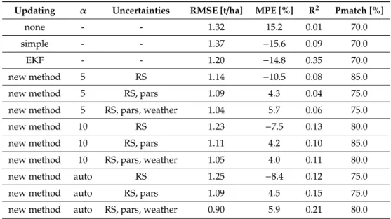
Table 3.Accuracies of the AquaCrop-OS field-level yield estimation on the validation dataset using different updating schemes. Uncertainties refer to the PDFs considered. RS: remote sensing; pars: parameter-related; weather: weather-related.

Updating α Uncertainties RMSE [t/ha] MPE [%] R2 Pmatch [%]

none - - 1.32 15.2 0.01 70.0

simple - - 1.37 −_15.6 _0.09 _70.0

EKF - - 1.20 −_14.8 _0.35 _70.0

new method 5 RS 1.14 −_10.5 _0.08 _85.0

new method 5 RS, pars 1.09 4.3 0.04 75.0

new method 5 RS, pars, weather 1.04 5.7 0.06 75.0

new method 10 RS 1.23 −_7.5 _0.13 _80.0

new method auto RS 1.25 −_8.4 _0.12 _75.0

new method auto RS, pars 1.09 4.5 0.15 75.0

new method auto RS, pars, weather 0.90 5.9 0.21 80.0

Our new PSO method performed similar to or better than the EKF with the twoαvalues of 5 and 10 when using all three uncertainties. Using only remote sensing inputs led to small changes in RMSE, but inverted the bias from positive to negative in all setups, similar to what we observed in the simple and EKF updates. Adding parameter-related uncertainties led to an improvement in both RMSE and MPE, while the subsequent addition of weather-related input affected results only slightly, and sometimes slightly deteriorated MPE. The adaptive version performed comparably and even outperformed the non-adaptive ones occasionally. Overall, when using all three uncertainties, model results improved by up to 0.42 t/ha in the RMSE, 11.2% in MPE, and 15% in terms of pmatch.

All versions of our approach were particularly successful in reducing bias. This is also apparent in the scatter plot in Figure7. It also indicates a tendency of the new method to reduce the range of predictions by avoiding low results<5 t/ha.

(16)

ISPRS Int. J. Geo-Inf.2020,9, 105 16 of 24 indicates a tendency of the model to overestimate yield. The simple updating scheme had no effect in terms of accuracy, but inverted the bias to an underestimation. The EKF performed better with a significant reduction of RMSE to 1.20 t/ha and a slightly smaller bias.

Table 3. Accuracies of the AquaCrop-OS field-level yield estimation on the validation dataset using different updating schemes. Uncertainties refer to the PDFs considered. RS: remote sensing; pars: parameter-related; weather: weather-related.

Updating α Uncertainties RMSE [t/ha] MPE [%] R² Pmatch [%] none - - 1.32 15.2 0.01 70.0 simple - - 1.37 −15.6 0.09 70.0 EKF - - 1.20 −14.8 0.35 70.0 new method 5 RS 1.14 −10.5 0.08 85.0

new method 10 RS 1.23 −7.5 0.13 80.0

new method auto RS 1.25 −8.4 0.12 75.0

new method auto RS, pars 1.09 4.5 0.15 75.0

Our new PSO method performed similar to or better than the EKF with the two 𝛼 values of 5 and 10 when using all three uncertainties. Using only remote sensing inputs led to small changes in RMSE, but inverted the bias from positive to negative in all setups, similar to what we observed in the simple and EKF updates. Adding parameter-related uncertainties led to an improvement in both RMSE and MPE, while the subsequent addition of weather-related input affected results only slightly, and sometimes slightly deteriorated MPE. The adaptive version performed comparably and even outperformed the non-adaptive ones occasionally. Overall, when using all three uncertainties, model results improved by up to 0.42 t/ha in the RMSE, 11.2% in MPE, and 15% in terms of pmatch.

All versions of our approach were particularly successful in reducing bias. This is also apparent in the scatter plot in Figure 7. It also indicates a tendency of the new method to reduce the range of predictions by avoiding low results < 5 t/ha.

Figure 7. Scatter plots of measured vs. predicted yield on the field-level for (left to right) simple update, EKF update, and the new method (adaptive; all three uncertainties).

3.2. Pixel-Level Yield Estimation

Table 4. Accuracies of AquaCrop-OS pixel-level yield estimation on the validation dataset using different updating schemes. Abbreviations as in Table 3.

Figure 7. Scatter plots of measured vs. predicted yield on the field-level for (lefttoright) simple update, EKF update, and the new method (adaptive; all three uncertainties).

3.2. Pixel-Level Yield Estimation

Table4shows that on the pixel-level, the model with no updating again produced a high RMSE and showed a bias of 12.7%. Both simple updating and the EKF inverted the bias to an underestimation of−_{14.9 % and}−_{13.3 %, respectively. Interestingly, both techniques increased the inaccuracies.}

Table 4. Accuracies of AquaCrop-OS pixel-level yield estimation on the validation dataset using different updating schemes. Abbreviations as in Table3.

none - - 1.52 12.7 0.08 65.6

simple - - 1.88 –14.9 0.07 43.8

EKF - - 1.79 –13.3 0.08 45.6

new method 1 RS 1.80 –12.9 0.06 43.6

new method 2 RS 1.72 –12.7 0.05 49.0

new method auto RS 1.82 –12.8 0.05 46.2

new method auto RS, pars 1.52 –2.9 0.07 59.7

The new method performed better when using remote sensing and parameter-related uncertainties, while adding weather-related uncertainty did not improve the results consistently. Still, even the best results only reduced the RMSE by about 0.09 t/ha. Despite that, it again managed to reduce the bias significantly. The adaptive version seemed to incorporate the different uncertainties more consistently, as indicated by decreasing RMSE and MPE with each added uncertainty. The scatter plot in Figure8

supports these findings. As previously mentioned, the new method reduced the bias through slightly higher predictions with a slightly smaller range.

(17)

Updating α Uncertainties RMSE [t/ha] MPE [%] R² Pmatch [%] none - - 1.52 12.7 0.08 65.6 simple - - 1.88 –14.9 0.07 43.8 EKF - - 1.79 –13.3 0.08 45.6 new method 1 RS 1.80 –12.9 0.06 43.6

new method 2 RS 1.72 –12.7 0.05 49.0

Table 4 shows that on the pixel-level, the model with no updating again produced a high RMSE and showed a bias of 12.7%. Both simple updating and the EKF inverted the bias to an underestimation of −14.9 % and −13.3 %, respectively. Interestingly, both techniques increased the inaccuracies.

The new method performed better when using remote sensing and parameter-related uncertainties, while adding weather-related uncertainty did not improve the results consistently. Still, even the best results only reduced the RMSE by about 0.09 t/ha. Despite that, it again managed to reduce the bias significantly. The adaptive version seemed to incorporate the different uncertainties more consistently, as indicated by decreasing RMSE and MPE with each added uncertainty. The scatter plot in Figure 8 supports these findings. As previously mentioned, the new method reduced the bias through slightly higher predictions with a slightly smaller range.

Figure 8. Scatter plots of measured vs. predicted yield on the pixel-level for (left to right) simple update, EKF update, and the new method (adaptive; all three uncertainties). To improve visual interpretation, we displayed only a subset of 400 data points.

3.3. Pixel-To-Field Aggregated Yield Estimation

Table 5. Accuracies of AquaCrop-OS yield estimation on the validation dataset aggregating pixel-level simulations to the field-pixel-level using different updating schemes. Abbreviations as in Table 3.

Updating α Uncertainties RMSE [t/ha] MPE [%] R² Pmatch [%] none - - 1.12 11.6 0.09 72.2 simple - - 1.36 –12.5 0.11 69.4 EKF - - 1.33 –13.3 0.09 61.1 new method 1 RS 1.27 –10.9 0.10 72.2

Figure 8.Scatter plots of measured vs. predicted yield on the pixel-level for (lefttoright) simple update, EKF update, and the new method (adaptive; all three uncertainties). To improve visual interpretation, we displayed only a subset of 400 data points.

3.3. Pixel-To-Field Aggregated Yield Estimation

In general, the aggregated results (Table5) are better than those on the pixel-level, indicating a benefit from aggregation. When compared to field-level results, however, differences become apparent. Without an update, the model produced better results on the aggregated than on the field-level, while the simple update showed no significant difference. The EKF, however, performed worse on aggregated scales than on field-wise runs, indicated by a higher RMSE. The new method, in comparison, provides similar or better results on the aggregated compared to the field-level and bias tended to be a bit smaller. Results for the different uncertainty setups generally behaved in accordance to the observations in previous sections. Compared to the model without updating, we observed only small improvements for all updating schemes. Again, the scatter plot in Figure9shows a smaller range, but also a reduction in bias in the predictions using the new method compared to simple updating and EKF.

Table 5.Accuracies of AquaCrop-OS yield estimation on the validation dataset aggregating pixel-level simulations to the field-level using different updating schemes. Abbreviations as in Table3.

none - - 1.12 11.6 0.09 72.2

simple - - 1.36 –12.5 0.11 69.4

EKF - - 1.33 –13.3 0.09 61.1

new method 1 RS 1.27 –10.9 0.10 72.2

new method 2 RS 1.26 –10.5 0.10 72.2