Coupling of Vortex Flows with Control Jets for Enhanced Mixing and Flame Holding in Supersonic Flows

University of Tennessee, Knoxville

Trace: Tennessee Research and Creative

Exchange

Doctoral Dissertations Graduate School

5-2018

Coupling of Vortex Flows with Control Jets for

Enhanced Mixing and Flame Holding in

Supersonic Flows

Thomas Paul Fetterhoff

University of Tennessee, [email protected]

This Dissertation is brought to you for free and open access by the Graduate School at Trace: Tennessee Research and Creative Exchange. It has been accepted for inclusion in Doctoral Dissertations by an authorized administrator of Trace: Tennessee Research and Creative Exchange. For more information, please [email protected].

Recommended Citation

Fetterhoff, Thomas Paul, "Coupling of Vortex Flows with Control Jets for Enhanced Mixing and Flame Holding in Supersonic Flows. " PhD diss., University of Tennessee, 2018.

To the Graduate Council:

I am submitting herewith a dissertation written by Thomas Paul Fetterhoff entitled "Coupling of Vortex Flows with Control Jets for Enhanced Mixing and Flame Holding in Supersonic Flows." I have examined the final electronic copy of this dissertation for form and content and recommend that it be accepted in partial fulfillment of the requirements for the degree of Doctor of Philosophy, with a major in Aerospace Engineering.

Ahmad D. Vakili, Major Professor We have read this dissertation and recommend its acceptance:

Reza Abedi, Trevor M. Moeller, Andrew Yu

Accepted for the Council: Dixie L. Thompson Vice Provost and Dean of the Graduate School (Original signatures are on file with official student records.)

Coupling of Vortex Flows with Control Jets for

Enhanced Mixing and Flame Holding in Supersonic

Flows

A Dissertation Presented for the

Doctor of Philosophy

Degree

The University of Tennessee, Knoxville

Thomas Paul Fetterhoff

May 2018

ii

Copyright © 2018 by Thomas Paul Fetterhoff All rights reserved.

iii

Acknowledgements

I would like to thank my advisor, Dr. Vakili, for his guidance and patience throughout this endeavor. In addition, I would like to thank the members of my

committee; Dr. Moeller, Dr. Abedi, and Dr. Yu for their advice during this research. I especially appreciate the efforts by Dr. Meganathan and Mahdi Boudaghi for their computational work in support of this effort. A special thanks to my friends and family who have patiently tolerated my inattentiveness during this undertaking.

iv

Abstract

This study presents results of innovative integration of passive and active flow physics to accomplish effective supersonic mixing. The study is continuing cavity flow control research in the supersonic wind tunnel at the University of Tennessee Space Institute (UTSI). Initially numerical simulations were employed in support of choosing and refining the experimental configuration designs. Mixing enhancement was achieved through innovative coupling of aerodynamics of corner vortex flows and cavity flow control jets. The two geometries were chosen for their potential to generate strong streamwise vortices, weaker shock losses, low drag, and cavity recirculation zones. Another consideration was that the two physically different concepts would be studied to provide better understanding of the innovative mixing. Jets, simulating fuel injection, were used for flow control provided through penetrations in the front face and side walls of the cavity. Flow visualization, dynamic pressure (sound pressure level) data are measured and PIV measurements are presented and compared with computational

predictions for several geometries. High frequency dynamic pressure data were recorded to determine the cavity flow acoustic patterns. Measurements were acquired by a digital data acquisition system from two dynamic pressure transducers, located at different locations on the floor of the cavity. PIV measurements of selected configurations were performed. Schlieren and PIV images, pressure spectra and 2-D PIV data obtained are used as a basis for understanding the flow processes involved and comparison for improving the overall mixing and penetration performance. Streamwise vortices were

v

generated using two different innovatively designed geometries, strategically located upstream of selected cavity configurations, including various jet arrangements,

simulating fuel flow and control. Both configurations tested developed relatively strong streamwise vortex flows and weakened or lofted shear layers, indicating that mixing was enhanced. The two configurations exhibited flow changes with the simulated fuel

injection. However, different injection arrangements by the simulated fuel jets resulted in different details in the flow fields and their resulting acoustic spectra. The resulting flow fields show improved potential for fuel flow mixing and increased penetration while amplifying or attenuating flow unsteadiness in the cavity.

vi

Table of Contents

Chapter 1: Introduction ... 1

Background ... 1

Previously Investigated Suppression Techniques ... 2

Dissertation Scope ... 5

Chapter 2: Literature Review ... 7

Cavity Classifications ... 7

Cavity Oscillations ... 10

Cavity Flow Control Techniques ... 15

Passive Cavity Flow Control ... 15

Active Cavity Flow Control ... 19

Cavity Enhanced Mixing and Flame Holding ... 23

State of the Art in Supersonic fuel injection and mixing ... 29

Chapter 3: Experimental Apparatus ... 31

Wind Tunnel ... 31

Schlieren ... 33

Acoustic Instrumentation ... 33

Particle Image Velocimetry (PIV) ... 35

Test Articles and Cavity Configurations... 38

vii

Introduction ... 46

Sources of Error and Uncertainty Analysis ... 47

Clean Tunnel ... 54

Schlieren Analysis. ... 58

Computational Predictions ... 59

PIV Measurements ... 62

PIV Images... 62

Average Velocity Uave ... 68

Average Velocity, Vave ... 74

Average Z Vorticity ... 79 Turbulence intensity... 84 Reynolds Stress ... 89 xy Reynold Stress ... 89 xx Reynolds Stress ... 94 yy Reynolds Stress ... 99 Acoustic Spectra ... 104 Summary ... 108

Chapter 5 Conclusions and Recommendations ... 110

Future Research ... 112

List of References ... 113

viii

List of Tables

Table 1. Effect of sub pixel interpolation resolution on velocity uncertainty [Meganathan 2005]. ... 54 Table 2. Oscillatory Modes of Cavity 2 ... 108

ix

List of Figures

Figure 1. Upstream Mass Injection Schematic (Active Cavity Flow Control Technique)

[Fowler 2010]... 3

Figure 2. Blockage with Sawtooth or Perforated Spoiler Schematic (Passive Cavity Flow Control Technique) [Fowler 2010]. ... 4

Figure 3. Rod in Crossflow Schematic (Passive Cavity Flow Control Technique) [Fowler 2010]. ... 4

Figure 4. Airfoil in Crossflow Schematic (Passive Cavity Flow Control Technique) [Fowler 2010]... 5

Figure 5. Upstream distributed jets and verticle rods flow control [Milne 2012]. ... 5

Figure 6. A Typical Rectangular Cavity with a Freestream Crossflow [Fowler 2010]. ... 8

Figure 7. Open Cavity Flow, L/D<10. [Pentovich et. Al 1993]. ... 8

Figure 8. Closed Cavity Flow, L/D>13. [Pentovich et. Al 1993]. ... 8

Figure 9. Transitional Cavity Flow, 10<L/D<13. [Pentovich et. Al 1993]. ... 9

Figure 10. Categories of Fluid Cavities. [Rockwell & Naudascher 1978]. ... 9

Figure 11. Cavity Pseudo-Piston Oscillation Cycle. [Heller & Bliss 1975]. ... 13

Figure 12. Simple analytical cavity model. [Heller & Bliss 1975]. ... 14

Figure 13. Modular Structure of the Slot in the Flat Plate. [Smith et. al 1990]. ... 17

Figure 14. Two Configurations of Pins Which Were Used Most Effectively to Suppress Acoustic Resonance in the Slot. [Smith et. al 1990]. ... 17

x

Figure 16. Schematic of the experimental setup. [Vakili & Gauthier 1994]. ... 20

Figure 17. Schematic of the distribution of holes for two mass-injection systems: ... 20

Figure 18. Cavity configuration [Houpt et. al 2018]. ... 22

Figure 19. Schlieren images for different injection rates [Houpt et. al 2018]. ... 22

Figure 20. Schematic of underexpanded transverse injection into supersonic flowfield [Gruber et. al 1995]. ... 24

Figure 21. Fuel injection behind a rearward facing ramp [Abbitt et.al 1993]. ... 25

Figure 22. Swept Ramp injector [Hartfield et .al 1994]. ... 26

Figure 23. Physical and aerodynamic ramp schematics [Fuller et. al 1998] ... 27

Figure 24. Experimental Schematic (dimensions are in mm) [Nenmeni & Yu 2002]. .... 27

Figure 25. Schlieren images of mixing between Mach 2 air stream and transverse fuel injection without (above) and with (below) the cavity for mixing enhancement [Nenmeni & Yu 2002]. ... 27

Figure 26. Schlieren flow image with and without cavity [Arial et. al 2015]. ... 28

Figure 27. Power Spectrum distribution, Power Spectrum (dB) vs Frequency (Hz) [Arial et. al 2015]. ... 29

Figure 28. Sketch of HSWT with Schlieren Setup [Fowler 2012] ... 34

Figure 29. Baseline cavity spectra [Milne 2012]. ... 35

Figure 30. HSWT with PIV Apparatus [Loewen 2008]. ... 36

Figure 31. Frame Straddling Exposure Technique [Thiemann 2013] ... 37

xi

Figure 33. Test article number 2, dimensions in inches. ... 42

Figure 34. 3d Printed leading edge Section for test article #1 ... 43

Figure 35. Test article assembled into the tunnel floorplate. ... 44

Figure 36. Tubing added to the bottom of the test article for blowing and dynamic pressure measurement. ... 44

Figure 37. Test article #1 mounted inside the test section. ... 45

Figure 38. Test article #2 mounted inside the test section. ... 45

Figure 39. A schematic of the cross-correlation process is shown [Meganathan 2005]... 50

Figure 40. Clean Tunnel Photograph [Fowler 2010]. ... 55

Figure 41. Clean Tunnel Acoustic Spectra [Fowler 2010]. ... 56

Figure 42. Clean Tunnel – Schlieren Mach waves analysis [Fowler 2010]. ... 57

Figure 43. Clean Tunnel – PIV velocity vectors [Fowler 2010]... 57

Figure 44. Schlieren photographs with and without blowing (note a slight tilt in the image, tunnel floor is horizontal). ... 58

Figure 45. CFD Predictions, Mach number contours and streamlines, with and without blowing. ... 60

Figure 46. Test Article Number 2 CFD Prediction with and without blowing... 61

Figure 47. Blowing Configurations for PIV analysis. ... 62

Figure 48. Test Article 1 Centerline PIV Images. The location of the leading and training edges of the flow device are located by the red arrows. The trailing edge of the cavity is not in view ... 64

xii

Figure 49. Test Article 1 Off-Center PIV Images. The location of the trailing edge of the flow device is indicated by the red arrows. The leading edge of the flow device and the training edge of the cavity are not in view. ... 65 Figure 50. Test Article 2 Centerline PIV Images. The leading and trailing edges of the

flow devise and the training edge of the cavity are indicated by the red arrows. ... 66 Figure 51. Test Article 2 Off-Centerline PIV Images. The leading and trailing edges of

the flow devise and the training edge of the cavity are indicated by the red arrows. 67 Figure 52. Test Article 1 Centerline PIV Uave in meters/second. The trailing edge of the flow control device/leading edge of the cavity is at 40mm. The trailing edge of the cavity is not in view. ... 70 Figure 53. Test Article 1 Off-Centerline PIV Uave, m/s. The trailing edge of the flow

control device/leading edge of the cavity is at 40mm. The trailing edge of the cavity is not in view. ... 71 Figure 54. Test Article 2 Centerline PIV Uave, m/s. The trailing edge of the flow control

device/leading edge of the cavity is at 40mm. The trailing edge of the cavity is at 95mm. ... 72 Figure 55. Test Article 2 Off-Centerline PIV Uave, m/s. The trailing edge of the flow

control device/leading edge of the cavity is at 40mm. The trailing edge of the cavity is at 95mm. ... 73

xiii

Figure 56. Test Article 1 Centerline PIV Vave, m/s. The trailing edge of the flow device/leading edge of the cavity is at 40mm. The trailing edge of the cavity is not in view. ... 75 Figure 57. Test Article 1 Off-Centerline PIV Vave, m/s. The trailing edge of the flow

control device/leading edge of the cavity is at 40mm. The trailing edge of the cavity is not in view. ... 76 Figure 58. Test Article 2 Centerline PIV Vave, m/s. The trailing edge of the flow control

device/leading edge of the cavity is at 40mm. The trailing edge of the cavity is at 95mm. ... 77 Figure 59. Test Article 2 Off-Centerline PIV Vave, m/s. The trailing edge of the flow

control device/leading edge of the cavity is at 40mm. The trailing edge of the cavity is at 95mm. ... 78 Figure 60. Test Article 1 Centerline PIV Zvorticity. The trailing edge of the flow control device/leading edge of the cavity is at 40mm. The trailing edge of the cavity is not in view. ... 80 Figure 61. Test Article 1 Off-Centerline PIV Zvorticity. The trailing edge of the control

device/leading edge of the cavity is at 40mm. The trailing edge of the cavity is not in view. ... 81 Figure 62. Test Article 2 Centerline PIV Zvorticity. The trailing edge of the flow control

device/leading edge of the cavity is at 40mm. The trailing edge of the cavity is at 95mm. ... 82

xiv

Figure 63. Test Article 2 Off-Centerline PIV Zvorticity. The trailing edge of the flow control device/leading edge of the cavity is at 40mm. The trailing edge of the cavity is at 95mm. ... 83 Figure 64. Test Article 1 Centerline PIV Turbulence Intensity. The trailing edge of the

flow control device/leading edge of the cavity is at 40mm. The trailing edge of the cavity is not in view. ... 85 Figure 65. Test Article 1 Off-Centerline PIV Turbulence Intensity. The trailing edge of

the flow control device/leading edge of the cavity is at 40mm. The trailing edge of the cavity is not in view. ... 86 Figure 66. Test Article 2 Centerline PIV Turbulence Intensity. The trailing edge of the

flow control device/leading edge of the cavity is at 40mm. The trailing edge of the cavity is at 95mm. ... 87 Figure 67. Test Article 2 Off-Centerline PIV Turbulence Intensity. The trailing edge of

the flow control device/leading edge of the cavity is at 40mm. The trailing edge of the cavity is at 95mm. ... 88 Figure 68. Test Article 1 Centerline PIV xy Reynolds Stress. The trailing edge of the

flow control device/leading edge of the cavity is at 40mm. The trailing edge of the cavity is not in view. ... 90 Figure 69. Test Article 1 Off-Centerline PIV xy Reynolds Stress. The trailing edge of the

flow control device/leading edge of the cavity is at 40mm. The trailing edge of the cavity is not in view. ... 91

xv

Figure 70. Test Article 2 Centerline PIV xy Reynolds Stress. The trailing edge of the flow control device/leading edge of the cavity is at 40mm. The trailing edge of the cavity is at 95mm. ... 92 Figure 71. Test Article 2 Off-Centerline PIV xy Reynolds Stress. The trailing edge of the

flow control device/leading edge of the cavity is at 40mm. The trailing edge of the cavity is at 95mm. ... 93 Figure 72. Test Article 1 Centerline PIV xx Reynolds Stress. The trailing edge of the

flow control device/leading edge of the cavity is at 40mm. The trailing edge of the cavity is not in view. ... 95 Figure 73. Test Article 1 Off-Centerline PIV xx Reynolds Stress. The trailing edge of the

flow control device/leading edge of the cavity is at 40mm. The trailing edge of the cavity is not in view. ... 96 Figure 74. Test Article 2 Centerline PIV xx Reynolds Stress. The trailing edge of the

flow control device/leading edge of the cavity is at 40mm. The trailing edge of the cavity is at 95mm. ... 97 Figure 75. Test Article 2 Off-Centerline PIV xx Reynolds Stress. The trailing edge of the

flow control device/leading edge of the cavity is at 40mm. The trailing edge of the cavity is at 95mm. ... 98 Figure 76. Test Article 1 Centerline PIV yy Reynolds Stress. The trailing edge of the

flow control device/leading edge of the cavity is at 40mm. The trailing edge of the cavity is not in view. ... 100

xvi

Figure 77. Test Article 1 Off-Centerline PIV yy Reynolds Stress. The trailing edge of the flow control device/leading edge of the cavity is at 40mm. The trailing edge of the cavity is not in view. ... 101 Figure 78. Test Article 2 Centerline PIV yy Reynolds Stress. The trailing edge of the

flow control device/leading edge of the cavity is at 40mm. The trailing edge of the cavity is at 95mm. ... 102 Figure 79. Test Article 2 Off-Centerline PIV yy Reynolds Stress. The trailing edge of the flow control device/leading edge of the cavity is at 40mm. The trailing edge of the cavity is at 95mm. ... 103 Figure 80. Acoustic Spectra Test Article 1, PSD (dB/Hz) vs Frequency (Hz). ... 105 Figure 81. Acoustic Spectra Test Article 2, PSD (dB/Hz) vs Frequency (Hz). ... 106 Figure 82. Acoustic Spectra Test Article 2, No Mean Flow, PSD (dB/Hz) vs Frequency

(Hz). ... 107

1

Chapter 1: Introduction

Background

The study of cavity flows is important in various industrial systems as a result of many aerodynamics engineering configurations and applications. The automotive and aerospace industries have a particular need to study these types of flows. In the

automotive industry optimizing the flow over wheel wells, open windows of passenger cabins and tractor and trailer combinations is crucial to noise free, low-drag and efficient systems. For example, the sound levels produced by pressure oscillations (buffeting effects) caused by an open window in a moving vehicle can result in occupant fatigue and potential deafening. In the aircraft industry the flow over bomb bays, landing gear bays, and other doors and cavities is important to the aircraft’s ability to perform its mission. Flow over weapons bays can drastically affect weapon separation, vehicle performance, and the structural life of aircraft components. A common problem in the flow over cavities is acoustic resonance generating large amplitude pressure fluctuations within the cavity. A number of researchers have studied various cavities [Heller & Bliss 1975, Vakili & Gauthier 1994, Fowler 2010, Milne 2012, Thiemann 2013, Plentovich et. al 1993, Rockwell and Naudascher 1978, Karamcheti 1955, Roshko 1955 and Rossiter 1966] and found that at resonance the cavity flow can have substantial effect on a system’s health. Various studies have also been performed to develop attenuating the cavity flow oscillations, as discussed later. This study seeks to advance the state of the art by innovatively applying cavity flow control techniques to improve fuel flow mixing

2

and penetration in supersonic flows, while controlling acoustic unsteadiness in such cavity configurations.

Previously Investigated Suppression Techniques

In general, past supersonic studies at the University of Tennessee have been to understand these flows and develop active damping techniques which can be exploited over a broad operational envelope. Studies at UTSI have focused on flow controls which modify boundary layer and the shear layer flows over the cavity.

Vakili and Gauthier [Vakili & Gauthier 1994] applied steady distributed mass injection through porous plates upstream of the cavity and obtained near complete suppression of the cavity oscillations. A schematic of this concept, depicting upstream mass injection, is provided as Figure 1. Implementation of such a technique has not been readily suited for broad application most likely due to the added complexity and weight. Continued research has been motivated by the desire to develop better understandings and flow control techniques with comparable results, but with much simpler

3

Figure 1. Upstream Mass Injection Schematic (Active Cavity Flow Control Technique) [Fowler 2010].

Passive suppression techniques offer less complexity. Early investigations include the use of upstream fences to attenuate the flow instabilities by modifying the shear layer. Figure 2 is a depiction of such a fence placed upstream of a cavity. Givogue et.. al [Givogue et. al 2011] investigated the use of two dimensional Cylinders to alter the resonant tones and shear layer. Figure 3 depicts the placement of a rod in the flow at the leading edge of the cavity. The shedding vortices interact with the cavity shear layer, altering the acoustic tones within the cavity. Figure 4 is a representation of an airfoil similarly placed within the flow field. In this study the horizontal rod provided the best performance. The airfoil produced separated flows and provided the best results at the highest negative angle of attack.

Milne [Milne 2010] and later Thiemann [Thiemann 2013] replaced distributed jets and two-dimensional cylinders with cylindrical rods placed vertically in the flow

4

controlled to make the resulting flow control process adaptive. Furthermore, rods could transport fluids internally for expanded flow control and functionality, beyond cavity flow control.

Figure 2. Blockage with Sawtooth or Perforated Spoiler Schematic (Passive Cavity Flow Control Technique) [Fowler 2010].

Figure 3. Rod in Crossflow Schematic (Passive Cavity Flow Control Technique) [Fowler 2010].

Cavity

Flow

Blockage (Sawtooth or Perforated Spoiler)

Cavity

Vortex Shedding Rod

Flow

5

Figure 4. Airfoil in Crossflow Schematic (Passive Cavity Flow Control Technique) [Fowler 2010].

Figure 5. Upstream distributed jets and verticle rods flow control [Milne 2012].

Dissertation Scope

This research study performed in this dissertation seeks to extend the state of the art in cavity flow control and apply it to Supersonic Combustion Ramjet (SCRAMJET) combustor fuel injection and flame holding. SCRAMJETs are characterized by having supersonic flow inside the combustors. In supersonic flow, mixing for combustion is limited by slow shear layer growth. To accomplish combustion in practical streamwise distances in SCRAMJETs, innovative fuel injection, mixing and flame holding

techniques are the focus of numerous research and development studies. This

Cavity

Flow

6

dissertation seeks to advance the state of the art by innovatively applying active and passive flow control techniques to improve fuel flow mixing and penetration while controlling acoustic unsteadiness in the cavity, using low loss configurations. Leading edge shapes are investigated for the creation of corner flows and vortex creation. Cavity shaping and blowing are utilized to minimize cavity oscillations and improve fuel mixing and distribution. Complimentary numerical studies were performed as well as validation experiments in the UTSI supersonic wind tunnel, (M = 1.85), to help improve the

geometry and flow path for better overall results. The author has conducted an

exhaustive literature search for more contemporary literature, with limited success. This is believed to be an indicator that the subject of this study is highly current and relevant to supersonic mixing applications. It may also be that some of the relevant research results are either proprietary or are just not disseminated due to sensitivity of this topic. The author also believes and anticipates that results of this work would establish a fundamental milestone in supersonic mixing enhancements.

7

Chapter 2: Literature Review

Cavity Classifications

There have been traditionally three methods for classifying cavity types. The first is by geometry. Figure 6 outlines the layout of a simple cavity in a crossflow. Here, deep cavities are cavities that are deeper than they are long. Shallow cavities have their longest dimension as length.

The second method of classification is based upon where the shear layer

reattaches [Plentovich et. al 1993]. In an open Cavity, shown in Figure 7, the shear layer separates at the leading edge and attaches again at the rear of the cavity. Closed cavities, Figure 8, are sufficiently shallow that the shear layer attaches to the bottom of the cavity floor before separating and exiting the cavity. Transitional cavities, Figure 9, lie in between these two and can be either open or closed.

The third method is based upon the type of oscillations that are maintained in the cavity. Rockwell and Naudascher [Rockwell & Naudascher 1978] classify these cavities as Fluid Dynamic, Fluid Resonant, and Fluid Elastic, see Figure 10. Fluid Dynamic oscillation are typical of flow that is unstable. Fluid Resonant cavity flows have strong resonant oscillations within the cavity. Fluid Elastic flows result from the coupling of the oscillations with a moving boundary within the cavity.

8

Figure 6. A Typical Rectangular Cavity with a Freestream Crossflow [Fowler 2010].

Figure 7. Open Cavity Flow, L/D<10. [Pentovich et. Al 1993].

9

Figure 9. Transitional Cavity Flow, 10<L/D<13. [Pentovich et. Al 1993].

10

Cavity Oscillations

Cavity oscillations are pressure, density, and velocity fluctuations that occur as flow travels over the open side of a cavity. These flow oscillations occur as the free shear layer develops unsteady interactions with the rear wall of the cavity which may develop resonance with the cavity acoustics.

In the 1950’s Karamcheti [Karamcheti 1955] studied flow over a wide variety of shallow cavities at Mach numbers up to 1.5. Karamcheti observed that flows with laminar upstream boundary layers emitted more intense sound levels than those with turbulent boundary layers. He also noted that when the length of the cavity was small enough that the shear layer transverses the cavity there was no sound emission from the cavity flow.

Roshko [Roshko 1955], while studying drag effects of various length to depth ratio cavities, noted the formation of vortices forming from the separated boundary layer impinging on the trailing edge causing a high-pressure zone.

Rossiter [Rossiter 1966] developed an empirical model for calculating the periodic cavity frequency (ƒ).

(1) 𝑓 =𝑈∞ (𝑚−𝑛) 𝐿(1

𝐾𝑣 +𝑀)

Where L is the cavity length, U∞ is the freestream velocity, M is the freestream

11

the phase delay between acoustic wave and new vortex, and m is the mode number for the cavity oscillations.

Rossiter’s equation was suitable for Mach numbers up to 1.5. Above Mach 1.5 there was an increasing error in the prediction. This error was due to the assumption that the cavity speed of sound was the same as the freestream speed of sound. Heller, Holmes and Covert [Heller et. al 1971] modified Rossiter’s Equation (1) to improve its accuracy above Mach 1.5 by assuming that the cavity speed of sound was the freestream recovery speed of sound. They introduced the non-dimensional cavity frequency, Strouhal number (St) [Heller et. al 1971], (2) 𝑆𝑡 = 𝑓𝐿 𝑈∞= (𝑚−𝑛) { 𝑀 [1+𝛾−1 2 𝑀2] 1 2 +1 𝐾𝑣}

where γ is the ratio of specific heats. This equation shows good agreement up to Mach number 3.2.

Bilanin and Covert [Bilanin & Covert 1993] modeled supersonic flow over a cavity using a vortex sheet and a noise source. Their model related the inflow and outflow at the rear of the cavity to fluctuations of the free shear layer that was

approximated by a vortex sheet. The interaction of the vortex sheet, the cavity trailing edge, the resulting inflow and outflow from the cavity excited the shear layer at the

12

leading edge. They modeled these interactions by a noise source at the trailing edge of the cavity. These fluctuations are the source of the acoustic radiation.

Heller and Bliss [Heller & Bliss 1975] observed, in a water tunnel, a six-step oscillation process resulting in inflow and outflow at the trailing edge caused by unsteady oscillations of the shear layer. Figure 11 outlines the progression of these unsteady oscillations.

From [Heller & Bliss 1975]

A. “The pressure wave from the previous trailing-edge disturbance reaches the front of the cavity and reflects. Another such wave, already reflected of the front wall, approaches the rear of the cavity. The shear layer is above the trailing edge, so the external flow cannot interact with the trailing edge to produce disturbances. Some fluid leaves the cavity.”

B. “The shear layer waveform travels rearward, reducing the height of the shear

layer above the trailing edge. A new compression wave begins to flow from the rear as the flow interacts with the trailing edge and fluid is added to the cavity. The front compression wave has reflected off the front wall and moves rearward nearly in phase with the shear layer displacement. The previous rearward wave has reached the training edge.”

C. “The wave reflected off the front wall continues to move rearward in phase with

13

14

at the rear of the cavity, forms a new forward traveling compression wave as the external flow impinges on the back of the cavity.”

D. “the newly generated forward traveling compression wave and the reflected,

rearward traveling compression wave meet and interact near the cavity center.”

E. “After the interaction, the waves continue in their receptive directions. The

external part of the forward traveling wave moves into the supersonic flow, thus causing it to be tipped more than the external flow Mach angle. The rearward wave moves in the same direction as the external flow and travels at subsonic speed relative to it. This subsonic relative speed explains why the rearward traveling wave stops at the shear layer. At the rear, the shear layer reaches the trailing-edge

height.”

F. “The shear layer is now above the trailing edge height. The wave generated at

the trailing edge approaches the front of the cavity, and the reflected wave nears the rear of the cavity. The next step is the same as A, and the oscillation cycle repeats.”

The inflow and outflow at the trailing edge can be modeled by a replacing the rear wall of the cavity with a pseudo piston as depicted in Figure 12.

15

Cavity Flow Control Techniques

Both active and passive cavity flow control techniques have been utilized to minimize the drag and acoustic oscillations found in cavity flows. Techniques that have been investigated are typically employed to affect the shear layer or the boundary layer upstream of the cavity. Passive methods that have been investigated are shaping of the leading and trailing walls of the cavity, or by placing objects like vortex generators, pins, rods, or airfoils upstream of the cavity. Active methods for suppression include blowing and suction techniques as well as movable upstream devices placed in the flow or boundary layer.

Passive Cavity Flow Control

After concluding that the different sound spectrums from two geometrically different size cavities with a common length over depth ratio was the result of upstream boundary layer differences, Rossiter [Rossiter 1966] investigated spoilers located at the leading edge of a cavity to alter the boundary layer. The largest spoiler had the largest effect on attenuating the larger scales of flow unsteadiness.

Heller and Bliss [Heller & Bliss 1975] and Zhang et.al [Zhang et. al 1998] investigated slanting the training edge of the cavity. Heller and Bliss [Heller & Bliss 1975] discovered that the slanting the trailing edge of the cavity allowed the shear layer to remain straight over the cavity and for the proper impingement angle at the trailing edge. Heller and Bliss [Heller & Bliss 1975] also investigated adding a detached cowl. The position of the detached cowl is critical. Placed properly the cowl creates a

low-16

pressure area between the cowl and the trailing edge of the cavity canceling out the effects of the mass addition and removal process.

Perng and Dolling [Perng and Dolling 1998] studied the effects of varying cavity dimensions and slotted, slanted and vented geometries on cavity oscillations. They found that vented and slotted walls had little effect.

Franke and Carr [Franke & Carr 1975] screened a variety of baffles and leading and trailing edge modifications in the water tunnel. They tested the most promising configurations in the wind tunnel. They found that the ramps could reduce the pressure oscillations and that frequencies were well predicted by the modified Rossiter’s equation.

Smith, Gutmark and Schadow [Smith et. al 1990] utilized multi-steps and pins extending into the supersonic flow to reduce the amplitude of the acoustic oscillations, see Figure 13. A maximum reduction of a factor of 5 was produced by the utilization of the pin profiles shown in Figure 14.

Franke and Sarno [Franke & Sarno 1990] studied static and pulsating fences and steady and pulsating flow injection. Static fences at the leading edge were the most effective suppressor.

Loewen [Loewen 2008] investigated the effects of a rod in a crossflow and found the suppression of cavity tones was primarily due to blockage and lofting effects from the rod.

17

Figure 13. Modular Structure of the Slot in the Flat Plate. [Smith et. al 1990].

Figure 14. Two Configurations of Pins Which Were Used Most Effectively to Suppress Acoustic Resonance in the Slot. [Smith et. al 1990].

18

Givogue, Fowler, and Vakili [Givogue et. al 2011] investigated the use of two dimensional cylinders to alter the resonant tones and shear layer. The experiment was designed to assess whether the unsteadiness attenuation accomplished was a shear layer lofting effect or due to high frequency vortex shedding in the wake. Their results clearly indicate that the changes in shear layer were due to wake lofting effects and not high frequency vortex shedding. The wake size and location of the wake have a direct effect on the initial reflected wave generation and feedback mechanisms that drive the high amplitude pressure pulses in the cavity.

Milne [Milne 2012] and Thiemann [Thiemann 2013] studied the use of vertical rods that were placed upstream of the cavity projecting into the flow, Figure 15. There were sixteen rod size and layout configurations tested. Configurations with staggered patterns distorted the vorticity in the shear layer more effectively, and these were more effective at suppression of the resonant acoustic tones in the cavity.

Peltier et.al [Peltier et.al 2013] investigated cavity response to oblique shocks generated upstream to simulate shock induced flow distortion like that caused by a forebody upstream of the inlet. They found that the cavity flow was unsteady and the shear layer displacement was increased when the shock generator was located is in the furthest upstream position.

19

Figure 15. Configuration 12, Pin Plate in Test Section [Thiemann 2013].

Active Cavity Flow Control

There have been a number of instigations of active flow control methods [Sarno and Franke 1994, Vakili & Gauthier 1994, Wolfe 1995, Lamp and Chokani 1997, and Arunajatesan et. al 2008]

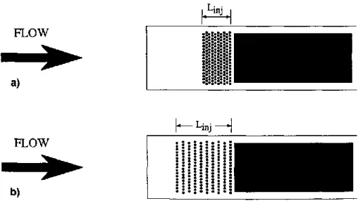
Vakili and Gauthier [Vakili & Gauthier 1994] studied the use of upstream mass injection through holes in plates located just upstream of the cavity, Figure 16. They achieved nearly complete suppression of the cavity oscillations with low density injection depicted in Figure 17. They attributed the effectiveness of this method to modifications to the shear layer instability characteristics.

20

Figure 16. Schematic of the experimental setup. [Vakili & Gauthier 1994].

Figure 17. Schematic of the distribution of holes for two mass-injection systems:

21

Wolfe [Wolfe 1995] found a correlation between the amount of mass injection and the effectiveness of the injection on suppression of acoustic tones in the cavity.

Arunajatesan et. al [Arunajatesan et. al 2008] compared the reduction in cavity acoustic resonance between blowing through slots or microjets at the leading edge of a cavity and the use of a fence the thickness of the boundary layer at the same location.

This study concluded that bowling concepts, using a small amount of mass injection, could be as effective as a leading-edge fence.

George, Ukeiley, Cattafesta and Taira [George et. al 2015] found that leading edge blowing through slots could reduce the acoustic resonance by as much as 40%.

Houpt et. al [Houpt et. al 2018] recently performed a study of Cavity-Based Flow Control in a Supersonic Duct Utilizing Q-DC Plasma Shock Wave Generator, in a Mach 2 flow with transverse fuel injection upstream of the cavity. They employed plasma generated oblique shocks from the opposite wall, so that the shocks impinged on the cavity shear layer at different positions, resulting in lifting the shear layer into the main stream, Figures 18 and 19. The lifting of the shear layer is expected to increase the mixing between the core flow and the cavity.

22

Figure 18. Cavity configuration [Houpt et. al 2018].

23

Cavity Enhanced Mixing and Flame Holding

In turbine engine augmentors and ramjet propulsion systems flame holding is normally accomplished by the use of bluff bodies in the flow field. These bluff bodies create recirculation zones in their wake. Fuel penetration and mixing is accomplished by the use of strut injectors across the flow field to distribute fuel across the airstream. In scramjet combustors these techniques create blockage and strong shock structures leading to high drag losses.

Fuel Injection and flame holding techniques for efficient combustion in scramjets has been the focus of ongoing research. Ben-Yakar and Hansen [Ben-Yakar and Hanson 2001] and Pandy and Sivasakthivel [Pandy and Sivasakthivel 2011] have conducted detailed reviews of recent advances.

A variety of fuel injection and flame holding schemes have been proposed and studied [Billig 1993, Abbitt et.al 1993, Hartfield 1994, Riggins 1995, Riggins and Vitt 1995, Curran et. al 1996, Tishkoff et. al 1997, Fuller et. al 1998, In et. al 1998, Sung et. al, 1999, Huber et. al 1979, Ben-Yakar and Hansen 1998, Hartfield et .al 1994, Curran 2001, Nenmeni & Yu 2002, Fry 2004, Gruber et. al 2004, Gruber et. al 2006, Tuttle et. al 2012, Grady et. al 2012, Tam 2012, Boles et.al 2012, Kirik et. al 2013, Barnes et. al 2014, and Arial et. al 2015].

As shown in Figure 20, early scramjet fuel injection was accomplished by injecting fuel transversely into the flow [Billig 1993, Gruber et. al 1995, and VanLerberghe 2000].

24

Figure 20. Schematic of underexpanded transverse injection into supersonic flowfield [Gruber et. al 1995].

25

In Figure 20 the upstream boundary layer separates and a normal shock is created causing this type of injection scheme to have high drag.

Abbitt et.al studied transverse injection behind a rearward facing step [Abbitt et.al 1993]. Here the expansion wave and shear layer interact with a bow shock created by the hydrogen fuel jets as shown in Figure 21.

Figure 21. Fuel injection behind a rearward facing ramp [Abbitt et.al 1993].

Hartfield, Hollo, and McDaniel [Hartfield et .al 1994] investigated vortex enhanced mixing behind a swept ramp injector Figure 22. The fuel injection was accomplished nearly parallel to the freestream flow. They found that the flow is turned away from the wall downstream by the ramp generated vortices, but the effect of the ramp generated vortices dissipates after 10 ramp height distances downstream, and that mixing rate decreases with increasing Mach number.

26

Figure 22. Swept Ramp injector [Hartfield et .al 1994].

Fuller et.al [Fuller et. al 1998] compared the effectiveness of ramp injectors to aerodynamic injectors, Figure 23. They found that the physical ramp injector reached fully mixed conditions in approximately half the length of the aerodynamic ramp but that the aerodynamic ramp had lower pressure losses.

Nenmeni and Yu [Nenmeni and Yu 2002] from the University of Maryland investigated cavity induced mixing in confined supersonic flows, Figure 24. Nenmeni and Yu [Nenmeni and Yu 2002] found that flow induced cavity resonance may be utilized to improve mixing over a broad array of cavity dimensions and Mach numbers, Figure 25.

Yu and Shadow, Sato et. al, and Arial et.al [Yu and Shadow1994, Sato et. al 1999, and Arial et.al 2015] investigated the interactions between cavities and fuel injection.

27

Figure 23. Physical and aerodynamic ramp schematics [Fuller et. al 1998]

Figure 24. Experimental Schematic (dimensions are in mm) [Nenmeni & Yu 2002].

Figure 25. Schlieren images of mixing between Mach 2 air stream and transverse fuel injection without (above) and with (below) the cavity for mixing

28

Arail, Sugano, Tsukazaki, and Sukaue [Arial et. al 2015] conducted research on the interactions between cavity flow and a ramp injector. In their study the cavity was placed on the opposite wall and upstream of the ramp injector. They found that the acoustic tones improved mixing of the fuel with the freestream flow. Figure 26 shows the improved fuel mixing in the presence of the cavity, and Figure 27 highlights the acoustic waves due to the cavity interacting with the fuel injection region.

Figure 26. Schlieren flow image with and without cavity [Arial et. al 2015].

Barnes, Tu, and Segal [Barnes et. al 2014] conducted research on the effect of mass injection in the cavity on flame holding capability and the mass exchange into the freestream. They injected flow into the cavity through the leading edge and compared that to injecting fuel at a rearward angle into the floor of the cavity. Both injection

29

locations created fuel rich regions interacting with vortices trapped in the cavity. The forward injection location resulted in a larger fuel rich zone in the cavity. They also found that the shear layer was entirely within flammability limits and would be a likely location for flame anchoring.

Figure 27. Power Spectrum distribution, Power Spectrum (dB) vs Frequency (Hz) [Arial et. al 2015].

State of the Art in Supersonic fuel injection and mixing

From the open literature, as shown in the above review, there are continuing efforts to facilitate efficient supersonic combustion through efficient fuel injection and mixing in short distances. Increased penetration into the cross flow has remained as the strongest challenge. Various sizes of struts with or without built in cavities are used to

30

increase fuel penetration and mixing into the main flow, but result in strong shocks and losses. Pulsed fuel injection if appropriately implemented, has been shown to help penetration and mixing away from the boundaries [Vakili et. al 1990, Vakili et. al 1994, Chang et. al 1995, and Williams 2016]. However, generating very high frequency pulsed fuel injections, needed for supersonic flows, is a challenge of its own.

This research is a first and introductory study of a new approach for increased fuel penetration for more efficient mixing in supersonic flow. Such a passive flow path design with distributed fuel injection for flow mixing control is new and represents a major step forwards in this developing field. Here we utilize passive geometry in coordination with strategically positioned fuel injection within a cavity to generate resonant cavity oscillations for increased local mixing coupled with passively generated streamwise vortices which help increase fuel rich flow mixing and penetration into the cross flow. This innovative approach, developed and improved based on flow physics, help to overcome the various challenges associated with supersonic fuel injection and mixing. The author believes and hopes that this work will establish a fundamental milestone in the direction of and state of the art for supersonic mixing enhancements.

31

Chapter 3: Experimental Apparatus

This experimental study was completed the 8 inch by 8 inch cross section supersonic blowdown wind tunnel in the Gas Dynamics Laboratory at the University of Tennessee Space Institute. Testing was completed on two different configurations designed to have low shock losses and to generate vorticial flows that enhance mixing. Instrumentation included Schlieren video, Particle Image Velocimetry (PIV), and high frequency pressure measurements.

Wind Tunnel

The University of Tennessee Space Institute wind tunnel is a blowdown wind tunnel. A schematic of the wind tunnel is provided as Figure 28. Air is compressed and stored in 18 High pressure cylinders at 3000 pounds per square inch. The tunnel

operation is controlled with LABView software. The air is routed to the wind tunnel plenum via a pneumatically driven flow control valve. In the plenum the flow is straightened by four stages of honeycomb and grid flow straighteners. The flow then travels through a convergent divergent nozzle designed for Mach 1.85. The nozzle has an axisymmetric entrance and an 8-inch by 8-inch square exit. The test section is 4 feet long with observation windows on the top and sides. The bottom has a removable floorplate where the test articles are mounted. The flow exits the test section and is expanded to atmospheric pressure through a diffuser.

The top window of the test section provides access for the Particle Image

Z-32

vorticity of the flow. The side windows of the test section provide a view of the test section for Schlieren imaging.

The stagnation temperature (T0) and stagnation pressure (P0) are measured in the

stilling chamber and the static pressure (P) is taken via static ports in the test section. The Mach number (M), static temperature (T), speed of sound (a), and freestream velocity (U∞) can be calculated using the following equations [National Advisory

Committee for Aeronautics (NACA) Report 1135]:

(3)                           1 1 2 1    p p M o (4) 2 2 1 1 M T T o    _ (5) a RT (6) 𝑈_∞= 𝑀𝑎

Where: T0=470.39 °R, P0=27.94 psi, P=4.58 psi, 1.4, and

lbf-ft 1716.49

slug-R

R _ _

 

Calculated Mach Number (M) = 1.84 Calculated Speed of Sound (a) = 821 ft./s Calculated Velocity in Test Section (U) = 1511 ft/s

33

Schlieren

The University of Tennessee Space Institute Schlieren system was installed in the test cabin so that the shock structure changes could be recorded via video camera. Schlieren is a flow visualization technique that relies on density changes in the flow field to be visualized due to the density changes in the flow leading to changes in refraction index. A sketch of the system is provided in Figure 28. A high intensity light sources is focused upon a concave mirror. The light is then reflected through the test section and onto another concave mirror. The image is then reflected off of a plane mirror and across a sharp edge and onto a screen. The image is then captured by a video camera and recorded and displayed in the wind tunnel control room.

Acoustic Instrumentation

High speed acoustic measurements were taken with Kulite® XCS-133-093-15D pressure sensors. These sensors were flush mounted to static pressure ports, located in the bottom floor of the test article cavity. Data was acquired at 40 kHz rates for several seconds for spectral analysis. Figure 29 provides a typical example of an acoustic

spectrum, along with the Rossiter Modes predicted by the modified Rossiter Equation, for the 11-inch cavity utilized by Milne [Milne 2012] in previous experimental studies at UTSI.

34

35

Figure 29. Baseline cavity spectra [Milne 2012].

Particle Image Velocimetry (PIV)

Particle Image Velocimetry (PIV) was used to provide an understanding of the flow vectors and vorticity in the region around the test article and above the tunnel floor. PIV uses a laser sheet to excite molecules that have been seeded into the flow upstream of the test section. This seed moves with the airflow and is assumed to have the same velocity vector as the airflow. When excited by the laser the molecule of seed fluoresces. The laser is pulsed, like a photographer’s flash, with very precise timing so that the

images can be compared. Since the time between the images is known, the change in the particles position allows the velocity vector to be calculated.

36

The seeding is comprised of 70% isopropyl alcohol, 30% water, with a small amount of fluorescein dye powder, nominal diameter of 2 micrometers. The fluid borne seed is injected into the tunnel flow using pressurized air via a coaxial tube in the convergent section of the nozzle.

The TSI LASERPULSE PIV system contains two neodymium-doped yttrium aluminum garnet (Nd:YAG) lasers. The beam is directed to the top of the test section through an articulated laser arm. This arm included a series of prisms and mirrors and finally the beams pass through spherical and cylindrical lenses creating a 0.04 inch by 4-inch laser sheet. This sheet is used to illuminate the leading-edge device and the forward portion of the cavity, Figure 30.

37

The TSI LASERPULSE PIV system utilizes INSIGHT™ PIV Software to operate the system components. INSIGHT utilizes a “frame straddling” procedure to create the two images that will be compared to generate the velocity vectors. This procedure compensates for the camera’s relatively low frame rates. The 1st laser pulse occurs near the end of the 1st camera exposure and the 2nd laser pulse occurs at the beginning of the second camera exposure, Figure 31. The time between the laser pulses (dT) is precisely controlled to 2 microseconds.

Figure 31. Frame Straddling Exposure Technique [Thiemann 2013]

The camera has a charge coupled device (CCD) with a sensor that has 1016 pixels high (y - from the tunnel floor toward the top of the test section), by 1000 pixels wide (x - in the flow direction). The INSIGHT PIV calibration procedures were followed []

resulting in a conversion factor of 115.60672 micrometers per pixel. Additional details concerning the TSI LASERPULSE PIV system and INSIGHT™ PIV Software operation, calibration and error analysis are included in references [Fowler 2010, Thiemann 2013, Loewen 2008, and Givogue et. al 2011].

38

After post processing of the data with Insight, the velocity vector data was

imported into Tecplot. Tecplot enabled the vector fields to be plotted and the vorticity in the z direction (ωz) to be plotted. The z direction is directed out of the side window of

the wind tunnel test section.

Test Articles and Cavity Configurations

Mixing in supersonic flows is limited by slow shear layer growth. Passive flow control techniques are typically the most robust in harsh environments like supersonic combustors. They are typically the best choice for enhancing fuel mixing in this type of environment.

Two test articles were developed. The test articles consisted of a vortex

generating shape on the leading edge of a cavity. Each had ports for air injection as well as for pressure measurements. The test articles configurations were developed to provide reduced acoustic signature and increased vorticity to provide mixing downstream of the cavity.

Two cavity and flow device configurations were chosen from a wider selection of configurations researched based on their potential mixing enhancement with lowest drag and shockwave losses. Additionally, these cavities were fitted with (simulated fuel) flow injection jets to accommodate this additional aspect of flow control. There were two jets located in the sidewall of the cavity, and three jets located in the front wall of the cavity.

39

The flow device and cavity geometries were innovatively designed to generate a relatively weak shock structure and thus have relatively low shock losses when compared with other flame holding and mixing schemes.

Independent CFD predictions were conducted by Dr. A.J. Meganathan in support of conceptual design and to predict the resulting flow fields. The CFD initially helped in minimizing the number of physical models which were fabricated and tested in the tunnel.

The two configurations and the experiments that resulted were specifically designed to provide a broad base information to assess the effectiveness of this novel concept. The two flow devices were selected to provide counter rotating vortices that would be lofted into the flow downstream. One was designed to concentrate the vorticity in the center of the cavity and the second was to concentrate the vorticity near the

sidewalls. One cavity was designed to maximize the pressure oscillations within the cavity and the second was designed to minimize them. The locations of the fuel injection ports were chosen to maximize interaction with the vortex flow structures.

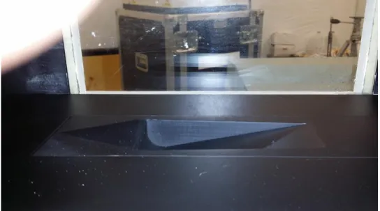
Test Article #1, Figure 32, had a pyramid like structure to generate vorticity just upstream of the cavity. This structure was designed to concentrate the vorticity in the center of the cavity. The cavity was slightly wider in the upstream than in the

downstream and the bottom of the forward edge of the cavity had a radius of 0.5 inches and the bottom of the cavity tapered to the trailing edge. The bottom of the cavity had three ports for high frequency pressure measurements. At the base of the pyramid were

40

three ports for blowing downstream with the direction of flow. These ports were

designed to change the shear layer location with respect to the cavity. There was also one port on each wall just down-stream of the cavity leading edge. These ports simulated injection ports that should enhance fuel mixing with the vortex structures coming into the cavity. This should enhance flame holding in the cavity and increase fuel penetration into the mean-flow downstream of the cavity. In this test article, the cavity was designed, with a tapered floor and rear cavity wall, to passively reduce the acoustic response.

Test Article #2, Figure 33, has a trapezoid ramp vortex generation device upstream of the cavity. The trapezoid is wider upstream and is the same width as the cavity at the trailing edge. This shape was chosen to concentrate vorticity near the cavity side walls. The cavity was nearly a square planform and is constant in depth. The cavity had an L/D of 4. There were 3 static pressure ports in the bottom of the cavity.

Like test article #1, at the base of the trapezoid ramp were three ports for blowing downstream with the direction of flow. These ports were designed to change the shear layer location with respect to the cavity. There was also one port on each wall just down-stream of the cavity leading edge. These ports simulated injection ports that should dampen the acoustics and enhance fuel mixing with the vortex structures coming into the cavity. This should enhance flame holding in the cavity and increase fuel penetration into the mean-flow downstream of the cavity.

41

42

43

The two test articles were constructed by a 3d printing process at the UTSI Gas Dynamics Laboratory. The parts were printed in sections and bolted together as can be seen in Figure 34. The parts were then shaped with filler and sanded to provide the proper surface finish. They were then painted and installed into the removable floorplate of the supersonic tunnel test section, Figure 35. Tubing was attached to the blowing and transducer ports in the cavity. The air supply for blowing was plumbed to the five tubes on the left side in Figure 36. The transducers were connected to the three tubing ports that are along the base of the cavity, shown on the right side in Figure 36. The test articles were then installed into the tunnel along with the floorplate, Figures 37 and 38

44

Figure 35. Test article assembled into the tunnel floorplate.

Figure 36. Tubing added to the bottom of the test article for blowing and dynamic pressure measurement.

45

Figure 37. Test article #1 mounted inside the test section.

46

Chapter 4: Results and Discussion

Introduction

In this chapter, the analysis of the data taken will be presented. The testing was conducted over a period of more than a year. Delays were caused by a number of higher priority tests, forcing interruptions in the availability of the wind tunnel. These

interruptions caused additional delays in the test program by requiring reinstallation and recalibration of test articles and data systems.

While there were compromises in the data systems and optics, the results are clear enough to generate conclusions concerning the flow control techniques in question. The Schlieren data was quantitatively analyzed to make quick assessments of blowing effectiveness. The PIV data was reduced and velocity, vorticity, turbulence, and

Reynolds Stress were calculated. Pressure data were analyzed to obtain spectra to help better understand the effects of the injected flow into the cavity on the flow field. The results will be discussed in the following sections.

Testing was completed with simulated fuel injection by blowing pressurized air through orifices in the cavity walls. In the following discussion the label “No Jets” indicates that none of the flow orifices in the cavity had flow, the label “Axial Jets” refers to blowing flow through the 3 jets at the forward face of the cavity, the label “Side Jets” indicates that blowing is occurring through the orifices in the side of the cavity near the front face, and “all Jets” refers to flow through both the axial and side orifices.

47

Sources of Error and Uncertainty Analysis

Typical sources of error include the equipment, equipment calibration, sampling, and processing algorithms. The facility and measurement systems were effectively the same as those used in previous experiments in the same UTSI supersonic wind tunnel. A full description of the statistical error analysis is provided in references [Fowler 2010, Thiemann 2013, Loewen 2008, and Wolfe 1995]. In the following paragraphs, some additional factors contributing to the uncertainty of the results are described.

Initial testing was completed with a Schlieren system. The Schlieren system was compromised in two ways. The first was the lack of adequate spacing for optimum mirror and screen spacing. The second compromise was inadequate light source intensity. The low intensity of the light source provided, resulted in low contrast and weak gradients, making the Schlieren images difficult to read and analyze. Another contributing factor was the presence of Mach waves in the test section of the tunnel test section.

PIV measurements were taken along the test unit centerline and along the side edge of the cavity. One difficulty in taking PIV measurements off of the test cell centerline is the ability to get adequate seeding of the flow off centerline. The seeding device is located in the plenum chamber on the cell centerline. This device consists of two concentric rods with an orifice on one side. The inner tube supplies the seed and the outer tube supplies blast air to atomize the seeding fluid. But since this rod is inserted at the tunnel centerline in the plenum, most of the seed is along the test section centerline.

48

To compensate for this fact the rod that supplied the seed was turned at an angle to the flow in an attempt to get additional seeding at the cavity edge. This technique had limited effect on the quality of seeding along cavity edge.

The camera used to acquire the PIV images was compromised due to the presence of a bad pixel. The inoperative pixel resulted in a line across the screen from the top to the bottom behind the cavity. This created a discontinuity in the data which can be seen in all of the PIV images and the results. Care must be taken to not mistake an artifact of this bad pixel for an actual flow phenomenon.

A number of different factors can contribute to increasing uncertainties and errors in pressures, Schlieren, and PIV measured data for calculating and generating flow field information. They can be broadly classified into errors associated with hardware and setup.These types of errors are related to the sensors, equipment component setup, acquisition and data analysis for the measured variables.

The Schlieren images obtained in this study were utilized as qualitative information and are used to detect relative changes in the flow field due to changes in model geometry and jets flow.

Pressure measurements are affected by details of pressure transducer’s

specifications such as accuracy and linearity; error band determined via calibration can be taken into account to estimate the overall order of accuracy for the measurement.

For the PIV data, the measurement system is composed of the laser beams with Gaussian profile in Transverse Electro Magnetic mode 00, which translate into laser light

49

sheets uniformity and alignment, CCD camera resolution, synchronizer for timing

between different frames, optical magnification is calibrated. Aberrations inherent in the optics govern the overall uncertainty in the PIV data. Even though most of these are carefully set up and selected for about one percent accuracy, the combined effects of the various factors increase the uncertainty to about 5%-10%, with the higher accuracy applicable to the higher speed ranges. In the PIV setup used for our measurements, there was a damaged pixel in the CCD chip. This resulted in a vertical line loss of data

corresponding to the bad pixel, in each image matrix, and resulted in contamination of the calculated data in the proximity of the line. Due to the averaging and interrogation sub window size of 32x32 pixels, this effect is evident in most processed data and images containing velocities, vorticity and stresses. Since the affected area is in the downstream of the cavity its effect is not detrimental to the understanding of the flow field. For this reason, the local patterns are generally not affecting the results and conclusions.

Electronics, including timing synchronization circuits are highly accurate. Therefore, the error in the timing is normally ignored for the flow speeds in this study. For a given flow field, using a camera with highest density CCD with a nominal dT, (or Del t), improves the accuracy of calculated particle displacements. Normally, a larger separation time is recommended, within the maximum feasible dT for a particular flow measurement equipment setup and a chosen interrogation window size.

Estimating errors in PIV measurements are affected by components resolutions, optical set up and data analysis methodology. The interrogation sub window size in this

50

study was 32 x 32 pixels including a 70 % overlap to increase the number of calculated vectors. Usually a 50% overlap related to the Nyquist criterion is used. Using a higher overlap only increases the number of vectors and not the scales that could be truly resolved. Finer resolution of velocity vectors help to improve calculations of vorticity and turbulence properties. The dynamic spatial range is basically fixed by the image size and interrogation spot size. The interrogation process is repeated to cover the entire image for each pairs of images. Detailed studies have shown that cross-correlation methods, Figure 39, perform much better than any other method in terms of signal-to-noise ratio and flexibility of choosing parameters for PIV imaging [Meganathan 2005].

Figure 39. A schematic of the cross-correlation process is shown [Meganathan 2005].

PIV is typically set up to provide a required spatial resolution, which is balanced between the size of the flow structures to be resolved with the interrogation spot size and image magnification. The setup used in this study was to resolve the shear layer and the flow near the boundary including its effects into the main flow.

51

The recorded size of particles on the image is usually larger than the particle size due to magnification. This increase in size comes from different parameters including diffraction limit of the recording optics and the experiment specific intensity of image [Adrian 1997]. This is only the optical effect and the actual image size is substantially larger than what is calculated (possibly up to an order of magnitude larger). For good spatial resolution displacement of particles due to the maximum gradient should be less than 5% of the interrogation spot size. Selecting the best dT between images and the best spot size (interrogation) is ideal for the expected upper flow velocities. Best practices established by various investigators limit the displacement due to the highest velocity be less than or equal to 25% of interrogation spot size.

Post processing of the raw vector field involves removal of the outliers using range, local median, standard deviation and mean filters, built into the PIV software. The eliminated vectors were filled through interpolation using Gaussian smoothing with exponent 1.3 [Meganathan 2005].

With the above considerations, all images were processed with an interrogation spot size of 32 x 32 pixels. The distance between any two adjacent vectors was 10 pixels. The calibration of the images was about 50 µm/pixel. The resolution of the vector map is 0.5 mm. In order to determine what minimum size vortex structures can be visualized, we have to decide how many data points are needed to determine a structure. When

measuring flow turbulence, to characterize mixing effects, the dynamic spatial range and the dynamic velocity range are more important than the spatial resolution [Adrian 1997].

52

These set the smallest size of the structures and the velocity fluctuations that would be resolved in a setup. The dynamic spatial range (DSR) is defined as the field-of view in the object space divided by the smallest resolvable spatial variation. [Adrian 1997]. The smallest resolvable scale is the smallest resolved particle displacement, which is due to with the maximum velocity.

The dynamic velocity range (DVR) is defined as the ratio of maximum velocity to the minimum resolvable velocity. Westerwheel [Westerwheel 1994, Westerwheel et.al 1997] estimates that usually the error in resolving the location of a correlation peak is in the order of 0.1 pixels. The capability of a PIV system to have both a large dynamic velocity range and a large spatial range is determined by the product of DSR and DVR, which is a constant for a given experimental setup. PIV systems having a large constant are best suited for turbulence research, and measurements in higher Reynolds number flows. [Abraham 2005, Adrian 1997] calculated the constant for a nearly similar set up as used in this study obtained approximate values of DSR = 200 and DVR = 40, resulting in a constant of about 8000, which would resolve velocities between 10 m/s - 300 m/s. This was for an assumed upper limit of image diameter of 10%, which will be improved to 1 m/s – 300 m/s, if 1% is used. This is important to be aware of for flows with a wide range of velocities [Meganathan 2005].

Experimental setup errors include calibration errors, non-optimal choice of tracer particles and laser sheet alignment [Meganathan 2005]. The need to choose ideal seeding materials and seeding dispersion system has already been discussed.

53

“Computational errors include truncation errors, detection errors, and precision errors. Truncation errors are very similar to truncation error in numerical analysis caused by approximations using numerical discretization. Most PIV algorithms use a simple forward differencing interrogation scheme in which the velocity at time t is calculated using particle images recorded at time t and t+del t. This approximation is accurate to the order of del t, and second order in space increments” [Meganathan 2005]. These errors are systemic and cannot be completely eliminated due to the inherent nature of image correlations. There also exist certain small errors due to correlations between random particles that are not the same pair which influence the peak-searching algorithm. Various data processing smoothing operations, including sub pixel interpolations introduce certain amount of errors. Particularly of importance is the higher % errors introduced into the lower speeds regions are in the flow field in the cavity or near the boundaries, from the high-speed regions of the flow.

Vorticity and stresses components are obtained by