NBER WORKING PAPER SERIES
CROSS-SECTIONAL TOBIN'S Q
Frederico Belo
Chen Xue
Lu Zhang
Working Paper 16336
http://www.nber.org/papers/w16336
NATIONAL BUREAU OF ECONOMIC RESEARCH
1050 Massachusetts Avenue
Cambridge, MA 02138
September 2010
For helpful comments, we thank Andrew Abel, Kerry Back, Gurdip Bakshi, Jonathan Berk, Mark
Flannery, Vito Gala, Eric Ghysels, Bob Goldstein, Rick Green, Burton Hollifield (UBC discussant),
Urban Jermann, Pete Kyle, Mark Loewenstein, Stavros Panageas, Jay Ritter, Paulo Rodrigues (EFA
discussant), Neng Wang, Toni Whited, and seminar participants at the 2010 CEPR/Studienzentrum
Gerzensee European Summer Symposium in Financial Markets, Duke University, the 2010 European
Finance Association Annual Meetings, Federal Reserve Bank of New York, McGill University, Michigan
State University, Rice University, Shanghai University of Finance and Economics, Tsinghua University,
the 2010 University of British Columbia Phillips, Hager and North Centre for Financial Research Summer
Finance Conference, University of Florida, University of Maryland, and University of Minnesota.
The portfolio data and the SAS and Matlab programs for the construction of the portfolio data and
GMM estimation and tests are available upon request. We are responsible for all the remaining errors.
The views expressed herein are those of the authors and do not necessarily reflect the views of the
National Bureau of Economic Research.
NBER working papers are circulated for discussion and comment purposes. They have not been
peer-reviewed or been subject to the review by the NBER Board of Directors that accompanies official
NBER publications.
Cross-sectional Tobin's Q
Frederico Belo, Chen Xue, and Lu Zhang
NBER Working Paper No. 16336
September 2010, Revised July 2011
JEL No. E22,G12,G14,G31
ABSTRACT
The neoclassical investment model matches cross-sectional asset prices both in first differences and
in levels. With ten book-to-market deciles as the testing portfolios, the investment model largely matches
the Tobin’s Q spread and the average return spread across the extreme deciles. The parameter estimates
imply low adjustment costs around 1.7% of sales. The model’s fit results from three aspects of our
econometric strategy: (i) We test the model at the portfolio level to alleviate the impact of measurement
errors; (ii) we match the first moment to mitigate the impact of temporal misalignment between asset
prices and investment; and (iii) we allow for nonlinear marginal costs of investment. Our evidence
suggests that any differences between the intrinsic value of equity and the market value of equity tend
to dissipate in the long run.
Frederico Belo
Carlson School of Management
University of Minnesota
3-137 CarlSMgmt
321 19th Avenue South
Minneapolis MN 55455
Chen Xue
Stephen M. Ross School of Business
University of Michigan
701 Tappan Street
Ann Arbor MI 48109
Lu Zhang
Fisher College of Business
The Ohio State University
760A Fisher Hall
2100 Neil Avenue
Columbus, OH 43210
and NBER
1
Introduction
What determines equity valuation? This economic question has immense practical importance. A vast literature in accounting has built on the dividend discounting model and the residual income model to tackle the valuation question (e.g., Ohlson (1995), Dechow, Hutton, and Sloan (1999), and Frankel and Lee (1998)). Widely practiced in the financial services industry, equity valuation is at the core of standard business school curriculum around the world, with many textbook treatments (e.g., Palepu and Healy (2008), Koller, Goedhart, and Wessles (2010), and Penman (2010)). Al-though the accounting models are conceptually sound, their implementation often involves ad hoc (and unrealistic) assumptions that seem to leave at least some room for an alternative approach.
In asset pricing, unlike the cross section of returns, the cross section of equity valuation is vir-tually a virgin territory. In particular, following the major breakthroughs of Cochrane (1991, 1996) and Berk, Green, and Naik (1999), investment-based asset pricing has experienced a period of rapid growth. However, the literature has so far focused exclusively on cross-sectional returns. Reflecting on the severe (and surprising) lack of valuation research in asset pricing, Cochrane (2011) writes:
“We have to answer the central question, what is the source ofprice variation?” “When did our field stop being ‘asset pricing’ and become ‘asset expected returning’ ? Why are betas exogenous? A lot of price variation comes from discount-factor news. What sense does it make to ‘explain’ expected returns by the covariation of expected return shocks with market market return shocks? Market-to-book ratios should be ourleft-hand vari-able, the thing we are trying toexplain, not a sorting characteristic for expected returns (p. 23, original emphasis).”
As a fundamental departure from the existing literature on cross-sectional asset pricing, we take a first stab at the important valuation question. Specifically, we develop the neoclassical investment theory as a valuation tool to understand the levels (Tobin’sQ) of cross-sectional asset prices, while maintaining a good fit for the first differences (stock returns). We incorporate corporate taxes,
leverage, and nonlinear marginal costs of investment into the baseline investment model of Cochrane (1991). The key valuation equation emerges under constant returns to scale: Tobin’s Q equals marginalq, which can be inferred from the investment data via a specified adjustment costs function. The model also predicts that stock returns equal (levered) investment returns, defined as the next-period’s marginal benefit of investment divided by the current-next-period’s marginal cost of investment. We use generalized methods of moments (GMM) to evaluate the model’s fit in matching the cross section of average Tobin’sQand the cross section of average stock returnssimultaneously across the book-to-market deciles. We use the book-to-market deciles because these portfolios exhibit a large spread in Tobin’sQ(the value spread) and a large spread in average returns (the value premium). We see at least three advantages of the investment-based structural approach to valuation over the traditional accounting-based approaches. First, the only input that the investment approach re-quires is the current-period’s investment-to-capital. As such, the investment approach relieves us of the burden of forecasting earnings or cash flows many years in the future, a task that is challenging but is necessary for the accounting models to work. Second, by equating Tobin’s Qdirectly to the marginal cost of investment, we do not need to take a stand on the discount rate. It is well known that the valuation estimates from the standard accounting models can be extremely sensitive to the assumed discount rate.1
Third, at least in principle, the parameter estimates from the structural ap-proach are technology-driven “deep” parameters, which should be invariant to changes in optimizing behavior and economic policy per Lucas (1976). As such, the structural parameters should be more stable than the non-structural parameters such as the discount rate in traditional valuation models. Our key finding is that the neoclassical investment model can match both the levels and the
1
For example, Lundholm and Sloan (2007, p. 193) lament: “None of the standard finance models provide estimates that describe the actual data very well. The discount rate that you use in your valuation has a large impact on the result, yet you will rarely feel very confident that the rate you have assumed in the right one. The best we can hope for is a good understanding of what the cost of capital represents and some ballpark range for what a reasonable estimate might be.” Alas, a reasonable discount rate estimate is elusive. Penman (2010, p. 666) write: “Compound the error in beta and the error in the risk premium and you have a considerable problem. The CAPM, even if true, is quite imprecise when applied. Let’s be honest with ourselves: No one knows what the market risk premium is. And adopting multifactor pricing models adds more risk premiums and betas to estimate. These models contain a strong element of smoke and mirrors.”
first differences of cross-sectional asset prices. When we use the investment model to match theQ
moments only, the model predicts a value spread of 2.83, which is about 94% of the value spread observed in the data, 3.01. Across the book-to-market deciles, the average magnitude of the model errors is 0.17, which is less than 11% of the average Tobin’s Q across the deciles, 1.58. A scatter plot of average predicted average Tobin’s Qin the model against average realized Tobin’sQin the data across the testing portfolios is largely aligned with the 45-degree line. Also, the model fits the value spread with low adjustment costs that amount to 1.61% of sales.
Adding expected return moments in the GMM does not affect the model’s fit on theQmoments. This fit on the levels is achieved without sacrificing a good fit on expected returns. The alpha of the high-minus-low decile is only−1.08% per annum, which is substantially smaller than the alphas from
the CAPM (14.61%), the Fama-French (1993) three-factor model (6.71%), and the Carhart (1997) four-factor model (6.82%). However, the average magnitude of the alphas across the book-to-market deciles in the investment model is 1.96%, which is smaller than that from the CAPM (4.53%), but larger than those from the Fama-French model (1.46%) and the Carhart model (1.50%).
The investment model also does a good job in matching theQlevels at the industry level. With the book-to-market quintiles within each industry as the testing portfolios, the average magnitude of theQerrors is 0.20, which is less than 11% of the Tobin’sQaveraged across the industries, 1.85. The model predicts a value spread of 1.69, which is about 85% of the value spread of 1.99 averaged across the industries. Because average Q is estimated more precisely than average returns, using the Q moments facilitates greatly the identification of the model’s parameters, and increases the power of the tests. These benefits are especially important at the more disaggregated industry level, in which expected returns are noisy. As such, we argue that cross-sectional valuation should be taken seriously as a new dimension of the data to discipline asset pricing models.
The neoclassical investment framework is originally developed to understand investment behav-ior, both at the aggregate level and at the firm level.2 The failure of this framework in matching
2
levels is well known in the literature on standard investment regressions, which in effect test the model in levels (e.g., Chirinko (1993)). Our key finding that the model matches the cross section of Tobin’s Q and the cross section of stock returns simultaneously might be somewhat surpris-ing. The crux lies in three aspects of our econometric approach. First, we conduct the estimation at the portfolio level, which mitigates the impact of measurement errors in Tobin’s Q and other characteristics, errors that are likely responsible for the empirical failure of investment regressions. Second, we explore whether investment is a sufficient statistic for average Tobin’s Q. Focus-ing only on the first moment alleviates the impact of any temporal misalignment between asset prices and investment that can arise from, for example, investment lags. Third, while investment regressions are derived under the standard assumption of quadratic adjustment costs, we allow the marginal cost of investment to be nonlinear. We show that this nonlinearity is crucial for the model’s fit. With standard quadratic adjustment costs, the model implied value spread is only 0.57, which is less than 19% of the value spread in the data. Intuitively, Tobin’sQ is only propor-tional to investment-to-capital in the quadratic model. With the nonlinearity, Tobin’sQ is convex in investment-to-capital. As such, for a given magnitude of spread in investment-to-capital, the convexity magnifies the investment spread so as to produce a larger spread in Tobin’sQ.3
Our central finding has important implications. Shiller (1989, 2000) argues that measurement errors in Tobin’s Q that are likely responsible for the failure of investment regressions can arise from the differences between the intrinsic value and the market value of equity (see also Bond and Cummins (2000)). Consistent with this view, alternativeQmeasures that do not rely on the market value of equity appear to perform better in investment regressions than market-basedQmeasures.4 Our evidence that the neoclassical investment model matches the cross section of average Tobin’s (1982), and Abel (1983), and applied by, among others, Summers (1981), Abel and Blanchard (1986), Fazzari, Hubbard, and Petersen (1988), Whited (1992), Erickson and Whited (2000), Abel and Eberly (2001), and Hall (2004).
3
Prior studies have shown that the nonlinearity in the marginal cost of investment is important for understanding quantity data and stock market data (e.g., Abel and Eberly (2001), Israelsen (2010), and Jermann (2010)). We add to this body of evidence using data on cross-sectional asset prices.
4
The alternativeQmeasures include estimates based on cash-flow forecasts (e.g., Abel and Blanchard (1986) and Gilchrist and Himmelberg (1995)), analyst forecasts of earnings growth (e.g., Cumins, Hassett, and Oliner (2006)), and bond prices (e.g., Philippon (2009)).
Q suggests that the market value of equity and investment data are well aligned on average, and that, at the minimum, the differences between the intrinsic value and the market value of equity are short lived and tend to dissipate in the long run.
The rest of the paper unfolds as follows. We present the investment model and derive its im-plications for cross-sectional Tobin’sQand stock returns in Section 2. We discuss econometric and data issues in Section 3, present the estimation results in 4, and conclude in Section 5.
2
The Model of the Firms
We specify a neoclassical model of investment to derive testable predictions for both Tobin’sQand expected stock returns in the cross section. Time is discrete and the horizon infinite. Firms choose costlessly adjustable inputs each period, while taking their prices as given, to maximize operating profits (revenues minus expenditures on these inputs). Taking the operating profits as given, firms optimally choose investment and debt to maximize the market value of equity.
The operating profits function for firm i at time t is Π(Kit, Xit), in which Kit is
capi-tal and Xit is a vector of exogenous aggregate and firm-specific shocks. We assume that the
firm has a Cobb-Douglas production function with constant returns to scale. This assump-tion implies that Π(Kit, Xit) = Kit∂Π(Kit, Xit)/∂Kit, and that the marginal product of capital,
∂Π(Kit, Xit)/∂Kit=κYit/Kit, in which κ is the capital’s share and Yit is sales.
Capital depreciates at an exogenous rate ofδit. We allowδitto be firm-specific and time-varying:
Kit+1 =Iit+ (1−δit)Kit, (1)
in which Iit is investment. Firms incur adjustment costs when investing. The adjustment costs
function, denoted Φ(Iit, Kit), is increasing and convex inIit, is decreasing in Kit, and has constant
returns to scale in Iit and Kit. We allow the marginal costs of investment to be nonlinear:
Φit≡Φ(Iit, Kit) = 1 ν η Iit Kit ν Kit, (2)
in which η >0 is the slope adjustment cost parameter and ν >1 is the curvature adjustment cost parameter. The case withν = 2 reduces to the standard quadratic functional form.5
We allow firms to finance investment with one-period debt. At the beginning of time t, firm
i issues an amount of debt, denoted Bit+1, which must be repaid at the beginning of time t+ 1. Let rB
it denote the gross corporate bond return onBit. We can write taxable corporate profits as
operating profits minus depreciation, adjustment costs, and interest expense: Π(Kit, Xit)−δitKit−
Φ(Iit, Kit)−(ritB−1)Bit. Letτt be the corporate tax rate. We define the payout of firmias:
Dit≡(1−τt)[Π(Kit, Xit)−Φ(Kit, Kit)]−Iit+Bit+1−ritBBit+τ δitKit+τt(ritB−1)Bit, (3)
in which τtδitKit is the depreciation tax shield andτt(ritB−1)Bit is the interest tax shield.
LetMt+1be the stochastic discount factor fromttot+1, which is correlated with the aggregate component of the productivity shock Xit. The firm chooses optimal capital investment and debt
to maximize the cum-dividend market value of equity:
Vit ≡ max {Iit+△t,Kit+△t+1,Bit+△t+1}∞△t=0 Et ∞ X △t=0 Mt+△tDit+△t , (4)
subject to a transversality condition given by limT→∞Et[Mt+TBit+T+1] = 0.
To express firm i’s equilibrium market value of equity and stock return as a function of ob-servable firm characteristics, we let Pit ≡Vit−Dit be the ex-dividend equity value and the firm’s
valuation ratio or Tobin’sQasQit ≡(Pit+Bit+1)/Kit+1. The first-order condition of maximizing equation (4) with respect toIit implies that:
Qit= 1 + (1−τt)ην Iit Kit ν−1 . (5) 5
We place the slope adjustment cost parameter η inside the parentheses of equation (2) to make the unit of η
independent of the curvature parameter. With a free curvature parameter, the mean of (Iit/Kit) ν
varies substantially with the curvature. The mean is very small when the curvature is high, and large whenν is low. As such, whenηis placed outside the parentheses as in Merz and Yashiv (2007), the point estimate ofηis affected by the large change in mean of (Iit/Kit)
ν
. In particular, its point estimate can vary substantially between zero and, when the curvature parameter is high, values greater than 10,000, causing stability problems in the estimation.
As such, Tobin’sQ is a nonlinear function of investment-to-capital, Iit/Kit.
In addition, combining the first-order conditions of maximizing equation (4) with respect toIit
and Kit+△t+1 implies thatEt[Mt+1rIit+1] = 1, in whichritI+1 is the investment return, defined as:
ritI+1 ≡ (1−τt+1) h κYit+1 Kit+1 + ν−1 ν ηIit+1 Kit+1 νi +δit+1τt+1+ (1−δit+1) 1 + (1−τt+1)ην Iit+1 Kit+1 ν−1 1 + (1−τt)ην Iit Kit ν−1 . (6) The first-order condition of maximizing equation (4) with respect to Bit+△t+1 implies that Et[Mt+1rBait+1] = 1, in which rBait+1 ≡ ritB+1 −(ritB+1 −1)τt+1 is the after-tax corporate bond re-turn. Let ritS+1 ≡ (Pit+1+Dit+1)/Pit be the stock return and wit ≡ Bit+1/(Pit+Bit+1) be the market leverage. Under constant returns to scale, the investment return is the weighted average of the stock return and the after-tax corporate bond return (see Liu, Whited, and Zhang (2009)):
rIit+1 =witrBait+1+ (1−wit)ritS+1. (7)
Equivalently, the stock return equals the levered investment return:
rSit+1= rI
it+1−witritBa+1 1−wit
. (8)
Equations (5) and (8) express firmi’s Tobin’sQand stock return as functions of firm characteristics, providing the key predictions that we test empirically. To a first approximation, stock returns can be viewed as the first differences of equity value. Examining equations (5) and (8) simultaneously allows us to evaluate the fit of the model in both the levels and the first differences of asset prices, providing a new cross-sectional test for the neoclassical investment model.
3
Econometric Methodology and Sample Construction
3.1 Econometric Methodology
3.1.1 Moment Conditions
We test if the average Tobin’sQobserved in the data equals the average Qpredicted in the model:
E " Qit− 1 + (1−τt)ην Iit Kit ν−1!# = 0. (9)
In addition, we test whether the average stock return equals the average levered investment return:
E " rSit+1− rIit+1−witritBa+1 1−wit # = 0. (10)
To construct a formal test, define the model errors from their empirical moments as:
eQi ≡ ET " Qit− 1 + (1−τt)ην Iit Kit ν−1!# , (11) eRi ≡ ET " ritS+1− ritI+1−witrBait+1 1−wit # , (12)
in whichET [·] is the sample mean of the series in brackets. We calleQi the averageQerror andeRi
the average return error. The key identification assumption for estimation and testing is that both model errors have a mean of zero, an assumption standard in most Euler equation tests.
To see where the model errors come from, we note that although equations (5) and (8) are exact relations, measurement errors in variables are likely to invalidate them in practice. For equation (5), measurement errors can arise from mismeasured components ofQthat are better observed by firms than by econometricians, such as the market value of debt and the replacement value of the capital stock. In addition, the intrinsic value of equity can diverge from the market value of equity (e.g., Erickson and Whited (2000) and Eberly, Rebelo, and Vincent (2011)). For equation (8), the model errors can arise because of measurement or specification errors: Marginal product of capital might not be proportional to sales-to-capital, and adjustment costs might not be given by equation (2).
3.1.2 Estimation Method
We estimate the model parameters,κ,η andν using one-stage GMM to minimize a weighted aver-age ofeQi , a weighted average ofeRi ,or a weighted average of botheQi andeRi . When the stock return and Tobin’sQmoments are estimated separately, we use the identity weighting matrix in one-stage GMM to preserve the economic structure of the testing portfolios, following Cochrane (1996). How-ever, eQi can often be larger than eRi by an order of magnitude. As such, when we estimate the expected return and Tobin’sQmoments simultaneously, we adjust the weighting matrix such that the weights for different sets of moments make their errors comparable in magnitude. Specifically, we multiply the Q moments by a factor of PiceR
i /Pi ecQi
, in which ecQi is portfolio i’s Q error
from estimating only theQmoments, and ecR
i is portfolioi’s expected return error from estimating
only the expected return moments. In most of our applications,PiceR i /Pi ecQi is about 0.10. Following the standard GMM procedure, we estimate the parameters, b ≡ (κ, η, ν), by
min-imizing a weighted combination of the sample moments, denoted by gT. The GMM objective
function is a weighted sum of squares of the model errors, g′TWgT, in which W is the
ad-justed identity matrix. Let D = ∂gT/∂b. We estimate S, a consistent estimate of the
variance-covariance matrix of the sample errors gT, with a standard Bartlett kernel with a window length
of three. The estimate of b, denoted ˆb, is asymptotically normal with variance-covariance ma-trix: var(bˆ) = 1
T(D′WD)−
1
D′WSWD(D′WD)−1
. To construct standard errors for individual model errors, we use var(gT) = T1
I−D(D′WD)−1D′WSI−D(D′WD)−1D′W′,which is the
variance-covariance matrix for gT. We follow Hansen (1982, lemma 4.1) to form a χ2 test that all
or a subset of the model errors are jointly zero: g′T[var(gT)]
+
gT ∼χ2(# moments−# parameters),
in which χ2
denotes the chi-square distribution, and the superscript + denotes pseudo-inversion. We conduct the estimation at the portfolio level, for several reasons. First, the use of portfolio level data significantly reduces the impact of the measurement errors in firm-level data that have plagued the empirical performance of the investment model in investment regressions. By
aggregating the firm-level data to the portfolio level, the impact of measurement errors, such as those related to unobserved firm-level fixed effects, is reduced. Second, because forming portfolios helps diversify residual variances, the expected return and Tobin’sQspreads are more reliable statistically across portfolios than across individual stocks. Finally, investment data at the portfolio level are smoother than firm-level data, consistent with the smooth adjustment costs function in equation (2).
3.1.3 Comparison with Prior Tests on the Neoclassical Investment Model
Cross-sectional Tobin’s Qis a new dimension of the data not explored in the prior literature. Al-though the Tobin’sQmoments in equation (9) are related to the investment Euler equation tested in, for example, Whited (1992) and Hall (2004), our test design exploits the information contained in stock valuation data. In contrast, investment Euler equation tests use only investment and cash flow data, but ignore stock prices. The expected return moments in equation (10) have been ex-plored in Liu, Whited, and Zhang (2009). We instead focus on the Tobin’sQmoments. As noted, understanding valuation in the cross section is an important economic question on its own. In addition, theQ moments help identify the adjustment cost parameters that are otherwise hard to pin down from noisy expected return moments, as we show later in Section 4.
Merz and Yashiv (2007) use the neoclassical investment model to study stock market valuation (see also Israelsen (2010)). We ask a different question: What accounts for the largecross-sectional difference in Tobin’s Q between value stocks and growth stocks? The cross section also contains more valuation information to provide more powerful tests. In addition, our valuation test has sev-eral advantages over the Merz-Yashiv test. Merz and Yashiv derive and test a valuation equation from combining the first-order conditions of maximizing the market value of equity with respect to
Iit and Kit+1. Using our notations, we can write their valuation equation as:
Qit = Et Mt+1 (1−τt+1) ∂Πit+1 ∂Kit+1 − ∂Φit+1 ∂Kit+1 +δit+1τt+1+ (1−δit+1) 1 + (1−τt+1) ∂Φit+1 ∂Iit+1 . (13)
To implement this valuation equation, Merz and Yashiv must parameterize the marginal product of capital and the stochastic discount factor, Mt+1 (as the inverse of the firm’s weighted average cost of capital). In contrast, we implement directly the Tobin’s Q equation (5), which is immune to the specification errors in the marginal product of capital and as well as those inMt+1.
The investment regression literature tests whether Tobin’s Q is a sufficient statistic of invest-ment. The investment regressions are often performed on Tobin’s Q with cash flow or lagged in-vestment as controls (e.g., Fazzari, Hubbard, and Petersen (1988) and Eberly, Rebelo, and Vincent (2011)). As surveyed by Chirinko (1993), the neoclassical investment model is typically rejected because the investment regressions produce very low goodness-of-fit coefficients. In addition, cash flow and lagged investment are often significant, even when Tobin’s Q is controlled for, whereas Tobin’s Qis insignificant, even when it is used alone.
Our econometric approach differs from the standard investment regressions in three aspects. First, as noted, we conduct the estimation at the portfolio level, which mitigates the impact of mea-surement errors in both Tobin’sQand other characteristics. Second, we test whether investment is a sufficient statistic foraverage Tobin’sQ. Focusing on the first moment only alleviates greatly the impact of year-fixed effects as well as the impact of any temporal misalignment between asset prices and investment. The temporal misalignment can arise because investment lags prevent high and medium frequency movements in asset prices to be reflected immediately in the investment data (e.g., Lettau and Ludvigson (2002)). Also, Tobin’sQdepends on both existing capital and available technologies yet to be installed, but investment depends only on currently installed technology. As a result, Tobin’s Q is too forward-looking relative to investment, causing investment to be more responsive toQat long horizons than at short horizons (e.g., Abel and Eberly (2002)). Third, we al-low the marginal cost of investment to be nonlinear in the estimation, while the standard investment regressions can be derived only under the assumption that the marginal cost of investment is linear.
3.2 Data
Our sample consists of all common stocks on NYSE, Amex, and Nasdaq from 1965 to 2008. The firm-level data are from the Center for Research in Security Prices (CRSP) monthly stock file and the annual Standard and Poor’s Compustat files. We delete firm-year observations with missing data or for which total assets, gross capital stock, or sales are either zero or negative. We include only firms with fiscal year ending in the second half of the calendar year. We also exclude firms with primary standard industrial classifications between 4900 and 4999 and between 6000 and 6999 because the neoclassical investment theory is unlikely to apply to regulated or financial firms.
3.2.1 Portfolio Definitions
We use ten book-to-market deciles from Fama and French (1993) as the main testing portfolios. We focus on these portfolios because book-to-market predicts cross-sectional returns and because these portfolios generate a large cross-sectional spread in Tobin’s Q. Following Fama and French, we sort all stocks on book-to-market equity at the end of June of year t into ten deciles based on the NYSE breakpoints for the fiscal year ending in the calendar yeart−1. Book-to-market equity
is book equity for the fiscal year ending int−1 divided by the market equity for December of year t−1.6 Firm-year observations with negative book equity are excluded. We calculate equal-weighted
annual returns from July of year t to June of year t+ 1 for the portfolios, which are rebalanced at the end of each June. We use equal-weighted portfolio returns because these returns present a higher hurdle for asset pricing models to pass than value-weighted returns.
The construction of the book-to-market deciles includes firms from different sectors of the econ-omy. As such, the construction ignores the fact that technologies (in particular, the capital’s shareκ
6
Following Fama and French (1993), we measure book equity as stockholder equity plus balance sheet deferred taxes (Compustat annual item TXDB if available) and investment tax credit (item ITCB if available) plus post-retirement benefit liabilities (item PRBA if available) minus the book value of preferred stock. Depending on data availability, we use redemption (item PSTKRV), liquidation (item PSTKL), or par value (item PSTK), to represent the book value of preferred stock. Stockholder equity is equal to Moody’s book equity (from Kenneth French’s Web site), the book value of common equity (item CEQ) plus the par value of preferred stock, or the book value of assets (item AT) minus total liabilities (item LT). The market value of common equity is the closing price per share (item PRCC F) times the number of common shares outstanding (item CSHO).
and the adjustment cost parametersηandν) might vary across industries. To alleviate this concern, we also perform an industry-level analysis by constructing five book-to-market quintiles within each industry. We examine quintiles instead of deciles in each industry to guarantee that each portfolio contains a sufficient number of firms to alleviate the impact of measurement errors in firm-level data. We construct the book-to-market quintiles within each industry following the Fama-French (1993) procedure. The only difference is that we use all firms within a given industry (not just NYSE firms) to construct the breakpoints because the number of NYSE firms in some industries is too small.
3.2.2 Variable Measurement and Timing Alignment
We largely follow Liu, Whited, and Zhang (2009) in measuring accounting variables and in aligning their timing with the timing of stock returns at the portfolio level. We make two adjustments. First, we equal-weight corporate bond returns for the testing portfolios to make the weighting scheme of bond returns consistent with that of stock returns. In contrast, Liu et al. value-weight bond returns. Second, we include in the sample all the firms with fiscal year ending in the second half of the calendar year. In contrast, Liu et al. only include firms with fiscal year ending in December. Our procedural change substantially enlarges the sample.
The capital stock, Kit, is gross property, plant, and equipment (Compustat annual item
PPEGT), and investment, Iit, is capital expenditures (item CAPX) minus sales of property, plant,
and equipment (item SPPE if available). The capital depreciation rate,δit, is the amount of
depre-ciation (item DP) divided by the capital stock. Output,Yit, is sales (item SALE). Total debt,Bit+1, is long-term debt (item DLTT) plus short term debt (item DLC). Market leverage, wit, is the ratio
of total debt to the sum of total debt and the market value of equity. We measure the tax rate,τt,
as the statutory corporate income tax (from the Commerce Clearing House, annual publications). The after-tax corporate bond returns, rBa
it+1, are computed from rBit+1 using the average of tax rates in year tandt+ 1. For the pre-tax corporate bond returns,rBit+1, we follow Blume, Lim, and Mackinlay (1998) to impute the credit ratings for firms with no rating data from Compustat (item
SPLTICRM), and then assign the corporate bond returns for a given credit rating (from Ibbotson Associates) to all the firms with the same credit ratings. Specifically, we first estimate an ordered probit model that relates credit ratings to observed explanatory variables using all the firms that have credit ratings data. We then use the fitted value to calculate the cutoff value for each credit rating. For firms without credit ratings we estimate their credit scores using the coefficients esti-mated from the ordered probit model and impute credit ratings by applying the cutoff values of different credit ratings. Finally, we assign the corporate bond returns for a given credit rating from Ibbotson Associates to all the firms with the same credit rating.7
The Compustat dateset records both stock and flow variables at the end of yeart. In the model, however, stock variables datedt are measured at the beginning of yeart, and flow variables dated
t are realized over the course of year t. To capture this timing difference, we take, for example, for the year 2003 any beginning-of-year stock variable (such asBi2003) from the 2002 balance sheet and any flow variable over the year (such asIi2003) from the 2003 income or cash flow statement.
We aggregate firm-level characteristics to portfolio-level characteristics as in Fama and French (1995). For example, Yit+1/Kit+1 is the sum of sales in year t+ 1 for all the firms in portfolio i formed in June of yeartdivided by the sum of capital stocks at the beginning of year t+ 1 for the same set of firms. Iit+1/Kit+1in the numerator of ritI+1 is the sum of investment in yeart+ 1 for all the firms in portfolioiformed in June of yeartdivided by the sum of capital stocks at the beginning of yeart+1 for the same set of firms. Iit/Kitin the denominator ofrIit+1is the sum of investment in yeartfor all the firms in portfolioiformed in June of yeartdivided by the sum of capital stocks at the beginning of yeartfor the same set of firms. Because the firm composition of portfolioichanges
7
The ordered probit model contains the following explanatory variables: interest coverage, the ratio of operating income after depreciation (Compustat annual item OIADP) plus interest expense (item XINT) to interest expense; the operating margin, the ratio of operating income before depreciation (item OIBDP) to sales (item SALE), long-term leverage, the ratio of long-term debt (item DLTT) to assets (item AT); total leverage, the ratio of long-term debt plus debt in current liabilities (item DLC) plus short-term borrowing (item BAST) to assets; the natural logarithm of the market value of equity (item PRCC C times item CSHO) deflated to 1973 by the consumer price index; and the market beta and residual volatility from the market regression. We estimate the beta and residual volatility for each firm in each calendar year with at least 200 daily returns from CRSP. We adjust for nonsynchronous trading with one leading and one lagged values of the market return.
from year to year due to annual rebalancing,Iit+1/Kit+1 in the numerator of ritI+1 is different from Iit+1/Kit+1 in the denominator ofritI+2. Other characteristics are aggregated analogously.
4
Estimation Results
We report the estimation results from the sample including all publicly traded firms in Section 4.1 and from industry-specific samples in Section 4.2.
4.1 Matching Average Tobin’s Q and Stock Returns in the Cross Section
4.1.1 Descriptive Tests
Table 1 reports the averages and standard deviations of stock returns, Tobin’s Q, and other ac-counting characteristics for each book-to-market decile as well as for the high-minus-low decile. We define the value spread as the Tobin’s Qof the low book-to-market (growth) decile minus the Tobin’s Q of the high book-to-market (value) decile.8
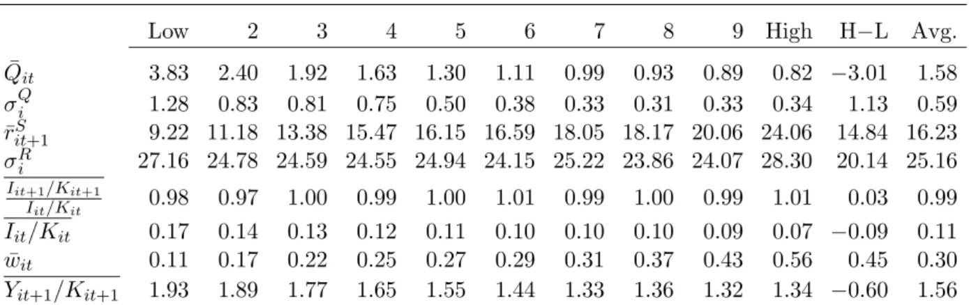
From the first row of the table, sorting on book-to-market equity produces a large value spread of 3.01 with a standard error of 1.13. We also observe a large spread of 14.84% per annum in the average equal-weighted return, which is more than 4.5 standard errors from zero. This large spread is a well established fact known as the value premium (e.g., Rosenberg, Reid, and Lanstein (1985)).
The volatility of Tobin’sQis, in relative terms, smaller than the volatility of stock returns. The annualized return volatility averaged across the deciles is 25.16%, which is more than 1.5 times the average return of 16.23% across the deciles. In contrast, the volatility of Tobin’sQaveraged across the deciles is 0.59, which is less than 40% of the average Tobin’s Q of 1.58. This evidence means that valuation moments are more precisely estimated in the data than expected return moments. As such, using the Qmoments in testing the investment model increases the power of the tests.
Equation (5) shows that Tobin’sQis an increasing function of the current investment-to-capital,
8Albeit related, our definition of the value spread differs from Cohen, Polk, and Vuolteenaho’s (2003). Cohen et
al. define the value spread as the log book-to-market equity of the value decile minus the log book-to-market equity of the growth decile. We adopt our definition based on the spread in Tobin’s Qbecause Qarises more naturally from the neoclassical investment model (see equation (5)).
Iit/Kit. Table 1 shows that consistent with the cross-sectional variation in Tobin’sQ, value firms
have lower current-period’s investment-to-capital on average than growth firms: 0.07 versus 0.17 per annum. Equations (6) and (8) provide a list of expected return components. The predicted stock re-turn in the model is increasing in the growth rate of investment-to-capital, (Iit+1/Kit+1)/(Iit/Kit),
market leverage, wit, and the next-period’s marginal product of capital, Yit+1/Kit+1, as well as decreasing in the current-period’s investment-to-capital, Iit/Kit. Table 1 also shows that value
firms have higher growth rates of investment-to-capital and higher market leverage than growth firms. These cross-sectional variations go in the right direction in accounting for the cross-sectional variation in expected stock returns. Going in the wrong direction, however, value firms also have lower next-period’s marginal product of capital than growth firms.
4.1.2 Point Estimates
Table 2 reports the point estimates and overall performance of the investment model using three sets of moments. In the Q column, we match average Tobin’s Q using moment condition (9). In ther column, we match average stock returns using moment condition (10). Finally, in theQ+r
column, we estimate the two sets of moment conditions jointly.
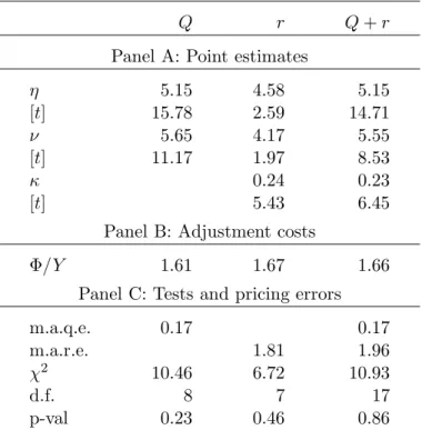
There are only three parameters in the model, the slope adjustment cost parameter, η, the curvature adjustment cost parameter,ν, and the capital’s share parameter,κ. Table 2 shows that the parameter estimates seem stable across the three sets of moments. Theη estimate ranges from 4.58 to 5.15, and is always significant. Theνestimate ranges from 4.17 to 5.65, and are significantly positive. In addition, theν estimates are significantly above two when theQmoments are used in the estimation. The evidence suggests that the adjustment costs function in the Tobin’s Q data exhibits more curvature than the standard quadratic functional form. The point estimates ofη and
ν also imply that the adjustment costs function is increasing and convex in investment-to-capital. The capital’s share parameter is estimated to be 0.24 when matching the expected return moments and 0.23 when matching both expected return and Tobin’sQmoments.
To interpret the magnitude of the adjustment costs, Table 2 reports the implied proportion of sales lost due to adjustment costs, computed as Φit/Yit= (ηIit/Kij)ν/(νYit). We calculate this
pro-portion by first computing the portfolio-level time series of realized adjustment costs-to-sales ratio and then averaging this ratio over time and across portfolios. The estimated magnitude of the ad-justment costs is small across all sets of moments. The adad-justment costs range from 1.61% (estimat-ing Tobin’sQmoments only) to 1.67% (estimating expected return moments only). These ratios are at the lower end of the empirical estimates surveyed in, for example, Hamermesh and Pfann (1996).
4.1.3 Overall Model Performance
Table 2 also reports three overall performance measures: the mean absolute Q errors (m.a.q.e.), the mean absolute return errors (m.a.r.e.), and the χ2
test. The m.a.q.e. and the m.a.r.e. are the means of the absolute errors across portfolios given by equations (11) and (12), respectively.
According to all three metrics, the investment model performs well in matching average returns and Tobin’s Q simultaneously across the testing portfolios. The m.a.q.e. is 0.17 both when we estimate the Tobin’s Qmoments only and when we estimate the expected return and Q moments jointly. These errors are small, representing less than 11% of the average Tobin’s Qof these port-folios (1.58, see Table 1). For expected returns, the m.a.r.e. ranges from 1.81% (matching expected return moments only) to 1.96% (matching expected return andQmoments jointly). These errors are also small, representing less than 12.5% of the average return of these portfolios (16.23%, see Table 1). The model is not rejected by theχ2
test across any set of moments, with p-values all above 20%.
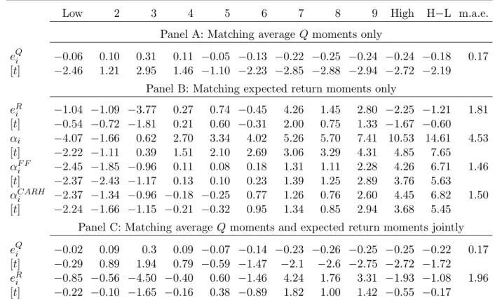
4.1.4 Individual Model Errors
The mean absolute errors and theχ2 test reported in Table 2 only indicate overall model perfor-mance. To provide a more complete picture of the fit, Table 3 reports the average Q errors from equation (11) and the expected return errors from equation (12) for all the individual portfolios, as well as their correspondingt-statistics. To put these expected return errors into perspective, we also report traditional asset pricing tests such as the CAPM, the Fama-French (1993) three-factor
model, and the Carhart (1997) four-factor model on the ten book-to-market deciles. The data for the factor returns and the risk-free rate are from Kenneth French’s Web site. We also report the mean absolute error for each model, computed as the mean of the absolute alphas across portfolios. Panel A in Table 3 reports the Q errors when we use the model to match the average Q mo-ments only. Even though the errors are economically small, with the average magnitude being less than 11% of the average Tobin’s Q across the deciles, most Q errors are more than two standard errors from zero. The significance of the model errors results from the fact that the Q moments are estimated precisely in the data. All the parameters and the moment conditions are estimated precisely. As such, even economically small errors lead to formal statistical rejections.
Panel B in Table 3 reports the expected return errors when the model is estimated to match average stock returns only. The model generates low model errors, and compares well with the performance from standard asset pricing models. Nine out of ten individual expected return errors are insignificant. The high-minus-low decile has an error of −1.21% per annum, which is
substan-tially lower in magnitude than the errors from the traditional models: 14.61% from the CAPM, 6.71% from the Fama-French model, and 6.82% from the Carhart model. The mean absolute error is 1.81% in the investment model, which is somewhat higher than 1.46% in the Fama-French model and 1.50% in the Carhart model, but lower than 4.53% in the CAPM.
Panel C in Table 3 reports the Tobin’s Q errors and the expected return errors when we use the model to match both sets of moments simultaneously. Overall, the model does a good job in matching the moments. Because of the lower precision of the stock return moments, all the moment conditions are less precisely estimated. As such, most of the individual Tobin’s Q errors are not significant. The Q error for the high-minus-low decile increases in magnitude slightly from−0.18
from Panel A to −0.22. However, the expected return error for the high-minus-low decile even
decreases somewhat in magnitude from −1.21% per annum in Panel B to −1.08%. The average
Q moments jointly with the expected return moments. The average magnitude of the expected return errors increases slightly from 1.81% when we estimate the expected return moments only to 1.96% when we estimate the expected return moments and the average Q moments jointly.
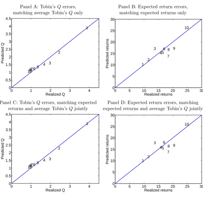
Figure 1 illustrates the investment model’s fit across different sets of moment conditions. We plot the average predicted Tobin’s Q against the average realized Tobin’sQ (Panels A and C), as well as the average levered investment returns against the average realized stock returns (Panels B and D) for the ten book-to-market deciles. If the model’s fit is perfect, all the scattered points should lie exactly on the 45-degree line. The figure shows that the scattered observations are largely aligned with the 45-degree line. In addition, comparing Panels A and C shows that the model’s fit on the average Q moments is robust to the addition of the expected return moments into the GMM estimation. Similarly, comparing Panels B and D shows that the model’s fit on the expected return moments is robust to the addition of the average Q moments into the GMM estimation. The bottomline is that the neoclassical investment model matches the data on cross-sectional asset prices not only in first-differences (stock returns), but also in levels (Tobin’s Q).
4.1.5 Parameter Stability
The model’s parameters are in principle “deep” structural parameters, describing the nature of production and capital adjustment technologies, which should be invariant to changes in optimizing behavior and economic policy per Lucas (1976). As such, any evidence of parameter instability would indicate specification and measurement errors in the model.9
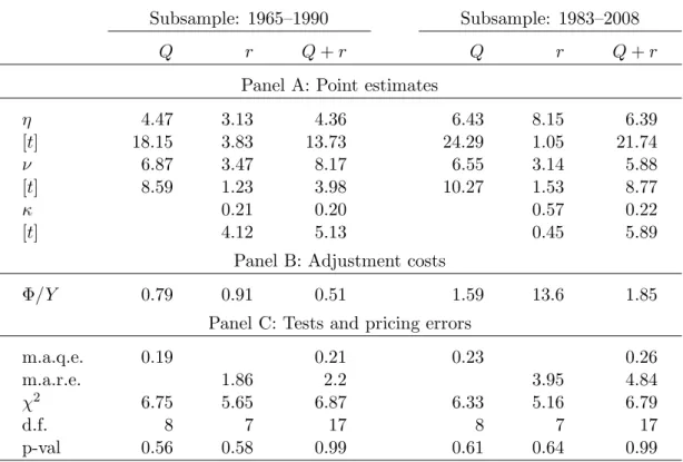
We study the stability of the parameter estimates in two ways, subsample analysis and recursive estimation. The main finding is that adding theQmoments in the estimation makes the parameter estimates more stable over time. Table 4 reports the GMM estimation and tests over two 25-year subsamples, with the testing portfolios formed annually in June based on book-to-market equity at the end of fiscal year ending
9
Although rarely discussed in the finance literature, such parameter instability in structural models is not uncommon in macroeconomics. For example, Oliner, Rudebusch, and Sichel (1996) show some parameter instability when estimating investment Euler equations. Fern´andez-Villaverde and Rubio-Ram´ırez (2007) find similar results when estimating dynamic stochastic general equilibrium models.
in calendar year from 1965 to 1989 and from 1983 to 2007. The table shows that the Tobin’s Q
moments seem important for identifying the structural parameters. The parameter estimates when we use the Tobin’sQmoments are more stable across subperiods. In particular, when only expected return moments are used, the capital’s share parameter,κ, is estimated to be 0.21 (t= 4.12) in the first subsample, but 0.57 (t= 0.45) in the second subsample. As such, the second estimate is less precise. In contrast, when we add the Tobin’sQ moments jointly with expected return moments, theκestimate varies from 0.20 to 0.22 across the two subsamples, witht-statistics both above five. Another indication of the parameter stability provided by theQmoments is the implied adjust-ment costs-to-sales ratio, Φ/Y. With only expected return moments, this implied ratio is 0.91% in the first subsample, but is 13.6% in the second subsample. Once we add the averageQmoments into the GMM estimation, the implied ratio varies only from 0.51% to 1.85% across the two subsamples. The increased stability reflects the fact that the Tobin’s Q moments are more precisely estimated than the expected return moments. In turn, this precision gives rise to the higher precision of the point estimates when we include the average Qmoments.10
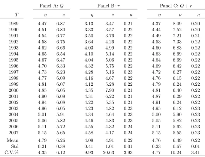
Table 5 provides further evidence on parameter stability by estimating the model recur-sively using a series of expanding windows. The expanding windows start from 1965. At year
T = 1989, . . . ,2007, we use all the accounting variables up to year T and stock returns up to year
T + 1 to estimate the model’s parameters. Table 5 reports the time series of the point estimates. From Panel A, the point estimates from matching average Q moments are stable. The slope ad-justment cost parameter, η, is on average 4.79 with a coefficient of variation (C.V., calculated as standard deviation divided by mean) of 4.35%. The curvature parameter, ν, is on average 6.26 with a C.V. of 6.12. From Panel B, estimating expected return moments only shows more time variation in the parameter estimates. In particular, the C.V. for theη parameter is 9.93%, and the
10
In untabulated results, we have experimented with halving the full sample by using the 1965–1987 and 1986–2008 subsamples. The averageQmoments play an even more important role in stabilizing the parameter estimates. With only expected return moments, theκestimate is 0.22 in the first subsample, but it hits the upper bound of one in the second subsample. Adding theQmoments brings theκestimate back to 0.24 in the second subsample.
C.V. for the ν parameter is 20.63%. Panel C shows that adding theQmoments more than halves the C.V.s of the estimates: The C.V. for theη estimate drops from 9.93% to 4.77%, and the C.V. for the ν estimate from 20.63% to 10.24%. Finally, with the terminal year of expanding windows starts from 1989, theκ estimates are stable with and without the Qmoments in the GMM.
4.1.6 The Role of Nonlinearity in the Marginal Cost of Investment
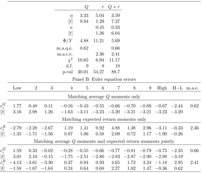
To quantify the importance of theν parameter for matching Tobin’sQ, we estimate the restricted version of the model with quadratic adjustment costs. In particular, we setν = 2 before choosing freely the η and κ parameters to minimize the GMM objective function. From Panel A of Table 6, the adjustment costs implied from the quadratic model are higher than those from the baseline model. In particular, the adjustment costs-to-sales ratio is 11.21% when estimating expected return moments only. The ratio is between 4–6% when theQmoments are included. The averageQerror is 0.62 when estimating the Q moments only and 0.66 when estimating the Q moments and the expected return moments jointly. In contrast, the averageQerror is only 0.17 in the baseline model. Panel B of Table 6 reports large errors for individual portfolios from the quadratic model. In par-ticular, when estimating theQmoments only, the model underpredicts the Tobin’sQof the growth decile by 1.77, and overpredicts that of the value decile by 0.67. As such, the model underpredicts the value spread by 2.44, which is more than 80% of the value spread (3.01) in the data! Panel A of Figure 2 confirms that the quadratic model fails miserably to match the value spread: The scatter plot is only slightly upward-sloping, deviating substantially from the 45-degree line. The fit on the
Qmoments from matching theQmoments and the expected return moments is largely similar (see Panel C of Figure 2). Finally, consistent with Liu, Whited, and Zhang (2009), the quadratic model matches well the expected return moments. The m.a.r.e. is only 2.36% per annum, and the error for the high-minus-low decile is 0.33%. Comparing Panels B and D in Figure 2 shows that including theQ moments into the estimation only deteriorates slightly the fit for the expected returns.
with quadratic adjustment costs, investment-to-capital is proportional to Tobin’s Q because the marginal cost of investment is linear in investment. With curvature, Q is a nonlinear function of investment. For a given magnitude of spread in investment-to-capital, the nonlinearity magnifies the investment-to-capital spread to produce a larger spread in Tobin’s Q.
4.2 Matching Expected Returns and Average Tobin’s Q Within Each Industry
We also ask whether the investment model can capture the value spread and the value premium at the more disaggregated industry level. Because the magnitudes of the value spread and the value premium exhibit some variation across industries, this extension provides an additional set of moments for the model to match. An additional benefit is that we allow the production and adjustment costs technologies to differ across industries.
4.2.1 Descriptive Tests
Using the Fama and French (1997) 17-industry classification, we test the investment model across the following industries: food, mines, oil, clothes, durables, chemicals, consumer, construction, steel, fabricated paper, machinery, cars, transportation, and retail. Out of the 17 industries, we exclude financials and utilities because these firms are not included in the main sample. In addition, we exclude the “other” industry because of its insufficient number of firms to form portfolios.
Table 7 reports the time series averages of selected characteristics of the book-to-market quin-tiles within each industry. We report the value premium, ¯rHS−L, the value spread, ¯QL−Q¯H, as well
as the m.a.r.e. and the high-minus-low alphas,αH−L, for the CAPM, Fama-French model and the
Carhart model for each industry. The value premium is positive across all the industries, but its magnitude shows some cross-industry variation. The value premium is high in the oil (17.34% per annum) and the chemicals (17.49%) industries, but is low in the car (2.94%) industry. The average value premium across all industries is 11.75%. The magnitude of the value spread also varies across the industries. It is high among the consumer goods industry (5.40) and low in the oil (0.77) and steel (0.86) industries. The average value spread across all industries is 1.99.
The average m.a.r.e. for the CAPM across the industries is 5.22% per annum. The CAPM alpha of the high-minus-low quintile, αH−L, is typically large (on average, 10.96%) and significant across
all but two industries. The average m.a.r.e. for the Fama-French model (4.12%) and the Carhart model (3.43%) are similar. Although smaller than the errors for the CAPM, the alphas of the high-minus-low quintile for the Fama-French and Carhart models are also large, with cross-industry averages being 6.91% and 6.53%, respectively, and are significant across many industries.
4.2.2 Point Estimates
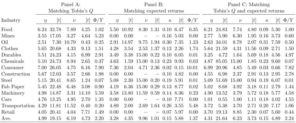
Panel A of Table 8 reports the parameter estimates and GMM tests when we use the investment model to match the averageQmoments of the book-to-market quintiles within each industry. The parameter estimates vary across industries and seem economically reasonable. The slope adjust-ment cost parameter, η, is significantly positive, and the curvature adjustment cost parameter,ν, is always above two. Confirming the results from the full cross section of firms, the importance of curvature for matching Tobin’sQis clear. The curvature parameter is estimated to be significantly above two across most industries. The implied magnitudes of adjustment costs are small across most industries. On average, the estimated adjustment costs represent about 2.20% of sales. The average adjustment costs are high in the consumer goods industry, about 7.90% of sales, and low in the steel and the oil industries, on average 0.07% and 0.25% of sales, respectively.
Panel B reports the parameter estimates and GMM tests when we match average stock returns of the book-to-market quintiles within each industry. In contrast with the results for the Tobin’sQ
moments, the parameter estimates are in general imprecisely estimated, and some estimates even take extreme values. The slope adjustment cost parameter, η, hits the lower bound of zero for four industries (mines, construction, cars, and retail). With η estimated to be zero, the curvature adjustment cost parameter,ν, is not identifiable from the expected return moments for these four industries. Theνestimate also hits the upper bound of 15 for four other industries (durables, chemi-cals, steel, and fabricated paper). Panel C reports the parameter estimates and GMM tests when we
use the investment model to match both average Tobin’sQ and average stock returns of the book-to-market quintiles within each industry. Because Tobin’sQmoments are included, the parameter estimates are precisely estimated. Theη parameter is estimated to be significantly positive across all but one industries. Theν parameter is estimated to be above two, except for the durables and car industries. The average adjustment costs continue to be low, on average about 2.24% of sales.
4.2.3 Overall Model Performance and Individual Model Errors
From Panel A of Table 9, the investment model produces small Q errors across all the industries when matching theQmoments. The cross-industry average m.a.q.e. is 0.20, which is slightly above 10% of the average value spread across the industries. TheQ errors for the high-minus-low quin-tile, eQH −eQL, are insignificant for all but three industries (oil, clothes, and steel). The model is
rejected by the χ2 test in only two out of the fourteen industries: oil and transportation. Given the parsimonious investment model with only one capital input, the rejection of the model across some industries is perhaps not surprising. For example, other inputs such as intangible capital or quasi-fixed labor (due to staggered labor contracts, for example) are omitted for parsimony, but these inputs can contribute to the measured Tobin’sQ. What is perhaps more surprising, at least to us, is the economically smallQerrors for many industries achieved by this parsimonious model. Figure 3 illustrates the good fit of the investment model in matching the Q moments in most industries. We plot the average predicted Tobin’sQagainst the average realized Tobin’sQfor the book-to-market quintiles. The portfolios are mostly aligned with the 45-degree line. The fit of the model is good in the clothes, durable goods, chemicals, construction, machinery and retail indus-tries, but is more modest in the mines, oil, steel, fabricated paper and transportation industries.
When the model is estimated to match the cross section of average stock returns, the model produces average model errors that are lower than those from standard asset pricing models. The average m.a.r.e. across industries is only 2.31% per annum in the investment model. This error compares favorably with the average pricing errors of the CAPM (5.22%), the Fama-French model
(4.12%), and the Carhart model (3.43%) (see Table 7). Also, all but two industries have insignificant expected return errors of the high-minus-low quintile (eRH −eRL) in the investment model.
The model produces small return and Q errors even when matching average Tobin’s Q and expected returns simultaneously. Both expected return errors and the Tobin’s Q errors increase somewhat, as expected, because the model is forced to match more moments. The m.a.r.e. increases from 2.31% (when matching return moments only) to 3.60%. These average return errors are still smaller in magnitude than the errors from the French model (4.12%), even though the Fama-French model is not required to match the Q moments. The average Tobin’s Q error increases somewhat, from 0.20 (when matching Tobin’s Qmoments only) to 0.25. Also, when both Tobin’s
Qand return moments are included, theχ2
test does not reject the model in any of the industries. Taken together, the industry level analysis provides robust evidence that the cross section of Tobin’s Q is a useful dimension of the data that should be taken seriously in estimating the neo-classical investment model. The cross section of average returns provides a set of moments that is imprecisely estimated. The imprecision is more severe when the tests are performed at the more disaggregated industry level, at which industry-specific idiosyncratic variance is not diversi-fied away. As a result, the statistical tests have lower power, and the moment conditions are not precise enough to identify the parameters. The low precision can also lead to extreme parameter estimates occasionally. Adding the Tobin’sQmoments in the estimation significantly increases the model’s ability to identify the structural parameters and the statistical power of the tests.
5
Conclusion
The neoclassical investment model matches cross-sectional asset prices both in first differences and inlevels simultaneously. When confronted with average Tobin’s Q and average stock returns mo-ments across the book-to-market deciles, the model predicts a Tobin’s Q spread of 2.79 and an average return spread of 15.92% per annum. The valuation error of 0.22 is about 7% of the Tobin’s
magnitude of the value premium (14.84%) observed in the data. The model matches these key mo-ments with reasonable parameter estimates for the production and capital adjustment technologies. In particular, the implied adjustment costs are low, about 1.66% of sales.
By providing the technological underpinnings of asset prices, our work has some implications on the popular view that the market value of equity often deviates from the intrinsic value of equity. In an endowment economy, because quantities are fixed, investor irrationality will fully impact on asset prices. At the other extreme, in a linear technologies economy without adjustment costs, investor irrationality will only impact on quantities through the optimal investment behavior of firms, leaving no trace in asset prices. The adjustment costs economy, which is what we model, lies somewhere in between the two extremes. Investor irrationality could put a short term dent on asset prices, but rational firms will eventually enter the economy, pay up adjustment costs, and flood any “fire” of asset pricing bubble with the “water” of investment. In the long run, the “water” extinguishes any impact of irrationality on asset prices. Our evidence seems consistent with this interpretation.
We view our work as a first step toward integrating asset pricing with the equity valuation and fundamental analysis literature in accounting. The quantitative results from the first step are en-couraging! Ultimately, valuation should be done at the firm level. Additional productive inputs such as labor and intangible assets should be incorporated into the neoclassical model. Nonconvex adjust-ment technologies that are likely relevant at the firm level should be incorporated as in, for example, Abel and Eberly (1994). More generally, a deep unification between asset pricing and the standard valuation framework in accounting (e.g., Koller, Goedhart, and Wessles (2010)) should be pursued.
References
Abel, Andrew B., 1983, Optimal investment under uncertainty, American Economic Review 73, 228–233.
Abel, Andrew B., and Olivier J. Blanchard, 1986, The present value of profits and cyclical movements in investment, Econometrica 54, 249–273.
Abel, Andrew B., and Janice C. Eberly, 1994, A unified model of investment under uncertainty, American Economic Review 84, 1369–1384.
Abel, Andrew B., and Janice C. Eberly, 2001, Investment and q with fixed costs: An empirical analysis, working paper, Northwestern University and University of Pennsylvania.
Abel, Andrew B., and Janice C. Eberly, 2002, Q for the long run, working paper, Northwestern University and University of Pennsylvania.
Berk, Jonathan B., Richard C. Green, and Vasant Naik, 1999, Optimal investment, growth options, and security returns,Journal of Finance 54, 1153–1607.
Blume, Marshall E., Felix Lim, and A. Craig MacKinlay, 1998, The declining credit quality of U.S. corporate debt: Myth or reality? Journal of Finance 53, 1389–1413.
Bond, Stephen R., and Jason G. Cummins, 2000, The stock market and investment in the new economy: Some tangible facts and intangible fictions,Brookings Papers on Economic Activity 1, 61–108.
Carhart, Mark M., 1997, On persistence in mutual fund performance, Journal of Finance 52, 57–82.
Chirinko, Robert S., 1993, Business fixed investment spending: Modeling strategies, empirical results, and policy implications, Journal of Economic Perspectives 31, 1875–1911.
Cochrane, John H., 1991, Production-based asset pricing and the link between stock returns and economic fluctuations, Journal of Finance 46, 209–237.
Cochrane, John H., 1996, A cross sectional test of an investment-based asset pricing model,Journal of Political Economy 104, 572–621.
Cochrane, John H., 2011, Discount rates, forthcoming,Journal of Finance.
Cohen, Randolph B., Christopher Polk, and Tuomo Vuolteenaho, 2003, The value spread,Journal of Finance 58, 609–641.
Cummins, Jason G., Kevin A. Hassett, and Stephen D. Oliner, 2006, Investment behavior, observable expectations, and internal funds,American Economic Review 96, 796–810. Dechow, Patricia M., Amy P. Hutton, and Richard G. Sloan, 1999, An empirical assessment of
the residual income valuation model,Journal of Accounting and Economics 26, 1–34. Eberly, Janice, Sergio Rebelo, and Nicolas Vincent, 2011, Investment and value: A neoclassical
Erickson, Timothy, and Toni M. Whited, 2000, Measurement error and the relationship between investment and q, Journal of Political Economy 108, 1027–1057.
Fama, Eugene F., and Kenneth R. French, 1993, Common risk factors in the returns on stocks and bonds,Journal of Financial Economics 33, 3–56.
Fama, Eugene F. and Kenneth R. French, 1995, Size and book-to-market factors in earnings and returns,Journal of Finance 50, 131–155.
Fama, Eugene F., and Kenneth R. French, 1997, Industry costs of equity, Journal of Financial Economics 43, 153–193.
Fazzari, Steven M., R. Glenn Hubbard, and Bruce C. Petersen, 1988, Financing constraints and corporate investment, Brookings Papers on Economic Activity 1, 141–195.
Fern´andez-Villaverde, Jes´us, and Juan F. Rubio-Ram´ırez, 2007, How structural are structural parameters? NBER Macroeconomic Annual 83–137.
Frankel, Richard, and Charles M. C. Lee, 1998, Accounting valuation, market expectation, and cross-sectional stock returns,Journal of Accounting and Economics 25, 283–319.
Gebhardt, William R., Charles M. C. Lee, and Bhaskaram Swaminathan, 2001, Toward an implied cost of capital,Journal of Accounting Research 39, 135–176.
Gilchrist, Simon, and Charles P. Himmelberg, 1995, Evidence on the role of cash flow for investment,Journal of Monetary Economics 36, 541–572.
Hall, Robert E., 2004, Measuring factor adjustment costs, Quarterly Journal of Economics 119, 899–927.
Hamermesh, Daniel S., and Gerard Pfann, 1996, Adjustment costs in factor demand, Journal of Economic Literature 34, 1264–1292.
Hansen, Lars Peter, 1982, Large sample properties of generalized method of moments estimators, Econometrica 40, 1029–1054.
Hayashi, Fumio, 1982, Tobin’s marginal q and average q: A neoclassical interpretation, Econometrica 50, 213–224.
Israelsen, Ryan D., 2010, Investment based valuation, working paper, Indiana University.
Jermann, Urban J., 2010, The equity premium implied by production, Journal of Financial Economics 98, 279–296.
Jorgenson, Dale W., 1963, Capital theory and investment behavior, American Economic Review 53, 247–259.
Koller, Tim, Marc Goedhart, and David Wessels, 2010, Valuation: Measuring and Managing the Value of Companies, 5th edition, John Wiley & Sons, Inc.
Lettau, Martin, and Sydney C. Ludvigson, 2002, Time-varying risk premia and the cost of capital: An alternative implication of the Q theory of investment, Journal of Monetary Economics 49, 31–66.
Liu, Laura Xiaolei, Toni M. Whited, and Lu Zhang, 2009, Investment-based expected stock returns,Journal of Political Economy 117, 1105–1139.
Lucas, Robert E. Jr., 1976, Econometric policy evaluation: A critique, Carnegie Rochester Conference Series on Public Policy 1, 19–46.
Lundholm, Russell J., and Rochard G. Sloan, 2007, Equity Valuation and Analysis, 2nd ed., McGraw-Hill Irwin.
Merz, Monika, and Eran Yashiv, 2007, Labor and the market value of the firm,American Economic Review 97, 1419–1431.
Ohlson, James A., 1995, Earnings, book values, and dividends in equity valuation,Contemporary Accounting Research 11, 661–687.
Oliner, Stephen D., Glenn D. Rudebusch, and Daniel Sichel, 1996, The Lucas critique revisited: Assessing the stability of empirical Euler equations for investment, Journal of Econometrics 70, 291–316.
Palepu, Krishna G., and Paul M. Healy, 2008, Business Analysis and Valuation: Using Financial Statements, 4th edition, South-Western.
Penman, Stephen H., 2010, Financial Statement Analysis and Security Valuation, 4th ed., McGraw-Hill Irwin.
Philippon, Thomas, 2009, The bond market’sq,Quarterly Journal of Economics 124, 1011–1056. Rosenberg, Barr, Kenneth Reid, and Ronald Lanstein, 1985, Persuasive evidence of market
inefficiency,Journal of Portfolio Management 11, 9–17.
Shiller, Robert J., 1989, Market volatility, Cambridge, Massachusetts: MIT Press.
Shiller, Robert J., 2000,Irrational exuberance, Princeton, New Jersey: Princeton University Press. Summers, Lawrence H., 1981, Taxation and corporate investment: Aq-theory approach,Brookings
Papers on Economic Activity 1, 67–127.
Tobin, James, 1969, A general equilibrium approach to monetary theory,Journal of Money, Credit, and Banking 1, 15–29.
Whited, Toni M., 1992, Debt, liquidity constraints, and corporate investment: Evidence from panel data,Journal of Finance 47, 1425–1460.
Table 1 : Descriptive Statistics of Ten Book-to-Market Deciles
For each book-to-market decile, we report the following statistics: the time series average, ¯Qit,
and the annualized standard deviation, σQi , of Tobin’s Q; the average stock return in annualized percent, ¯rS
it+1; the annualized volatility in percent of stock return, σRi ; the average growth rate
of investment-to-capital from time t and t+ 1, Iit+1/Kit+1
Iit/Kit ; the average investment-to-capital at t, Iit/Kit; the average market leverage, ¯wi; and the average sales-to-capital over t+ 1, Yit+1/Kit+1. The H−L is the high-minus-low book-to-market decile, and Avg. is the averages across deciles.
Low 2 3 4 5 6 7 8 9 High H−L Avg.
¯ Qit 3.83 2.40 1.92 1.63 1.30 1.11 0.99 0.93 0.89 0.82 −3.01 1.58 σQi 1.28 0.83 0.81 0.75 0.50 0.38 0.33 0.31 0.33 0.34 1.13 0.59 ¯ ritS+1 9.22 11.18 13.38 15.47 16.15 16.59 18.05 18.17 20.06 24.06 14.84 16.23 σRi 27.16 24.78 24.59 24.55 24.94 24.15 25.22 23.86 24.07 28.30 20.14 25.16 Iit+1/Kit+1 Iit/Kit 0.98 0.97 1.00 0.99 1.00 1.01 0.99 1.00 0.99 1.01 0.03 0.99 Iit/Kit 0.17 0.14 0.13 0.12 0.11 0.10 0.10 0.10 0.09 0.07 −0.09 0.11 ¯ wit 0.11 0.17 0.22 0.25 0.27 0.29 0.31 0.37 0.43 0.56 0.45 0.30 Yit+1/Kit+1 1.93 1.89 1.77 1.65 1.55 1.44 1.33 1.36 1.32 1.34 −0.60 1.56
Table 2 : Parameter Estimates and Tests of Overidentification
The table reports the estimation results via GMM on the Tobin’s Q moments and the expected return moments given by equations (9) and (10), respectively, using ten book-to-market deciles as the testing portfolios. κ is the capital’s share, η is the slope adjustment cost parameter, and ν is the curvature adjustment cost parameter. The t-statistics, denoted [t], test that a given estimate equals zero. Φ/Y is the ratio (in percent) of the implied capital adjustment costs-to-sales ratio. m.a.r.e. is the mean absolute return error in percent, and m.a.q.e. is the mean absolute valuation error. χ2
, d.f., and p-val are the statistic, the degrees of freedom, and the p-value testing that all the errors are jointly zero. TheQ column is for estimating the Qmoments only, ther column for estimating the expected return moments only, and theQ+rcolumn for estimating theQmoments and expected return moments jointly.
Q r Q+r
Panel A: Point estimates
η 5.15 4.58 5.15 [t] 15.78 2.59 14.71 ν 5.65 4.17 5.55 [t] 11.17 1.97 8.53 κ 0.24 0.23 [t] 5.43 6.45
Panel B: Adjustment costs
Φ/Y 1.61 1.67 1.66
Panel C: Tests and pricing errors