Ensemble Models for Spoofing Detection in Automatic Speaker Verification
Bhusan Chettri
1, Daniel Stoller
1, Veronica Morfi
1, Marco A. Mart´ınez Ram´ırez
1,
Emmanouil Benetos
1, Bob L. Sturm
21
School of EECS, Queen Mary University of London, United Kingdom
2School of EECS, KTH Royal Institute of Engineering, Stockholm, Sweden
Abstract
Detecting spoofing attempts of automatic speaker verification (ASV) systems is challenging, especially when using only one modelling approach. For robustness, we use both deep neural networks and traditional machine learning models and combine them as ensemble models through logistic regression. They are trained to detect logical access (LA) and physical access (PA) attacks on the dataset released as part of the ASV Spoofing and Countermeasures Challenge 2019. We propose dataset parti-tions that ensure different attack types are present during train-ing and validation to improve system robustness. Our ensemble model outperforms all our single models and the baselines from the challenge for both attack types. We investigate why some models on the PA dataset strongly outperform others and find that spoofed recordings in the dataset tend to have longer si-lences at the end than genuine ones. By removing them, the PA task becomes much more challenging, with the tandem detec-tion cost funcdetec-tion (t-DCF) of our best single model rising from 0.1672 to 0.5018 and equal error rate (EER) increasing from 5.98% to 19.8% on the development set.
Index Terms: ASVspoof 2019, logical access attack, physical access attack, countermeasures, anti-spoofing, model ensemble.
1. Introduction
An automatic speaker verification (ASV) [1] system aims at ver-ifying the claimed identity of a speaker and is widely used for person authentication. Though the technology has matured im-mensely over the past few years, studies [2, 3] have confirmed its vulnerability in the face of spoofing, also known as a presen-tation attack [4]. Mimicry [5], replay [6], text-to-speech (TTS) [3] and voice-conversion (VC) [2] technology are commonly used to perform logical access (LA) or physical access (PA) spoofing attacks in ASV systems [7]. While LA attacks (TTS and VC) are mounted by injecting synthetic/converted speech directly into the ASV pipeline bypassing its microphone, PA attacks (replay and mimicry), on the contrary, involve physical transmission of impersonated or playback speech through the systems’ microphone.
Spoofing countermeasures for reliable speaker verification are therefore of paramount interest. To this end, the ASV com-munity has released standard spoofing datasets [8, 9, 7] as part of the automatic speaker verification spoofing and countermea-sures challenges (ASVspoof), promoting research in this direc-tion. The ASVspoof 2019 challenge [10, 7] combines both LA and PA (excluding mimicry) attacks using the latest state-of-the-art TTS and VC methods and controlled-simulation setup EB is supported by RAEng Research Fellowship RF/128 and a Tur-ing Fellowship. DS is funded by EPSRC grant EP/L01632X/1. This research was supported by an NVIDIA GPU Grant.
for replay attacks, in contrast to the 2015 and 2017 spoofing datasets.
Designing a single model to robustly detect unseen spoofing attacks can be challenging, as demonstrated at the ASVspoof 2015 and 2017 challenges, where the best performing systems [11, 12, 13, 14, 15, 16] made use of an ensemble model com-bining features or scores. In this paper, we investigate LA and PA spoofing detection on the ASVspoof 2019 dataset using en-semble models. Below we summarise our contributions.
• We build our models by discarding data points (Sec-tion 2) ensuring non-overlap in spoofing condi(Sec-tions be-tween training and validation for better generalisation. • We demonstrate that combining information from deep
and traditional machine learning approaches along with our dataset partition can improve model generalisation. • We find that spoofed audio recordings for the PA task
tend to have more silence at the end than bonafide recordings. We perform three different interventions proving that models exploit this fault in the dataset and achieve lower performance without these cues.
• We make our dataset partition details and silence re-moval scripts available online1.
Our results suggest that performance metrics reported on the current PA dataset may be overestimating the actual per-formance of the models, which might become somewhat of a “horse” [17] that trivially sidesteps the actual problem, thus raising concerns about model validity as well as performance results. Prior work has addressed a similar issue of silence on the ASVspoof 2017 PA dataset [18], which calls for careful de-sign and validation of the 2019 PA spoofing dataset2.
2. Task description and dataset
Given a speech recording the task is to build a spoofing coun-termeasure, a model, to automatically determine whether it is a bonafide (genuine) or spoofed, either generated through TTS, VC or a replayed recording.The ASVspoof 2019 LA and PA datasets were released as part of this year’s challenge [10]. Both consist of8male and
12female speakers in the training and development subsets. In LA, there are2,580bonafide and22,800spoofed utterances in the training set and2,548bonafide and22,296spoofed ut-terances in the development set. In PA, both the training and development sets has5,400bonafide utterances, and48,600
and24,300spoofed utterances in the training and development sets, respectively. The evaluation set has around80,000and
135,000test utterances in the LA and PA datasets [7, 10].
1https://github.com/BhusanChettri/ASVspoof2019/ 2We have reported the “silence” issue to the challenge organisers.
The training and development subsets have similar spoofing algorithms/conditions in both the LA and PA datasets. We argue that using the same types of spoofing attacks during training and validation might lead to overfitting and poor generalisation on unseen attack conditions. Thus, we further partition the original training and development datasets for both LA and PA, ensur-ing non-overlap in spoofensur-ing attack conditions. We use a subset train trof the training set for model training and take a sub-set of the development (dev) sub-set and partition it intodev esfor model validation and early stopping anddev lrto build model ensembles through logistic regression. Although taking these subsets requires discarding many samples, it allows us to test how well a model generalises to previously unseen attack con-ditions: The spoofing attack conditions and speakers intrain tr anddev esare non-overlapping. Indev lr, we use all spoofing conditions of the dev set but discard speakers that have been used indev es.
3. Models in the Proposed Ensembles
In this section, we describe the approach used to design coun-termeasures for the LA and PA tasks of the ASVspoof 2019 challenge. A model ensemble is used in order to combine infor-mation from different countermeasure models employing vari-ous features and training procedures. This diversity leads to a powerful ensemble with good generalisation.3.1. Deep models
We train five deep models using raw audio or time-frequency representations as input to minimise a binary cross-entropy (CE) loss with an Adam optimiser and early stopping with a patience ofP epochs. As the dataset has more spoofed examples, we replicate the bonafide examples to ensure each batch contains an equal number of bonafide and spoofed exam-ples, which helps stabilise the training. At inference time, we use the output layer sigmoid activation as a score. We provide model-specific training details below.
3.1.1. Convolutional Neural Network (CNN)
We use the CNN architecture from [19], featuring 50% dropout in the fully connected layers, a batch size of32, and a learning rate of10−4
. We train the model for100epochs with an early stopping patience ofP = 5andP = 2for the LA and PA tasks, respectively. We use an utterance-level mean-variance normal-ized log spectrogram3, computed using a 1024-point FFT with
a hop size of 160 samples, as the input. For each task, we train two such CNN models, model A and B, on the first and last 4 seconds of each audio sample. We truncate or loop the spectro-gram time frames to obtain a unified time representation. 3.1.2. Convolutional Recurrent Neural Network (CRNN) We use a modified version of the CRNN architecture from our prior work [20] (model C). We train the model for500epochs with early stopping patience ofP = 10for both the LA and PA tasks. As input, we use a mean-variance (computed ontrain tr
set) normalized log-Mel spectrogram of 40Mel bands, com-puted on the first 5 seconds of truncated or looped audio sam-ples, using a 1024-point FFT with a hop size of 256 samples. During training, we use a batch size of8and32for the LA and PA tasks, respectively, with an initial learning rate of10−5that
3Power-spectrogram for the LA task and Mel-spectrogram with 80
mel bands (for computational reasons) for the PA task.
is halved on validation loss plateau with a patience ofP = 5
epochs, until10−8.
3.1.3. 1D-Convolutional Neural Network
We use the network architecture from the sample-level 1D CNN [21] (model D). In total, the model consists of9ReSE-2blocks [22]. These blocks are a combination of ResNets [23] and SENets[24]. We use the multi-level feature aggregation, where the outputs of the last three blocks are concatenated and fol-lowed by a fully connected layer of1024units, batch normal-ization and ReLU layers, a 50% dropout layer and a fully con-nected layer of1unit with sigmoid activation. Each convolu-tional layer has filters of size3,L2weight regularizer of0.0005
and all strides are of unit value. The raw audio input is3.7 sec-onds in duration and randomly sampled segments of this size are selected from the recordings. We loop shorter samples to obtain a unified time representation. We train the model using a batch size of16, learning rate of10−4and an early stopping patience ofP= 25epochs.
3.1.4. Wave-U-Net
We use a modified version of the Wave-U-Net [25], with five layers of stride four, and without upsampling blocks (model E). The outputs of the last convolution are max-pooled across time, reducing the parameter count and incorporating the in-tuition that the important features in the tasks are temporally local. Finally, we apply a fully connected layer with a single output to yield a classification probability. We train the model using a batch size of64, a learning rate of 10−5 and early stopping patience ofP = 10for both the LA and PA tasks, where an epoch is defined as 500 update steps. To ensure the audio inputs have the same length, we pad all recordings with silence to196608audio samples (= 12.23seconds). For the PA task, we also match real samples to their spoofed versions based on the speaker identity and utterance. We train on pairs of audio samples (discarding samples without any matches) and balanced batches, in order to stabilise the training process and improve generalisation by preventing the network from using speaker identity and utterance content for discrimination.
3.2. Shallow models
Additional to deep models, we use two different shallow [26] models: Gaussian Mixture Models (GMMs) and Support Vector Machines (SVMs).
3.2.1. GMM
We train three GMM models using60-dimensional static, delta and acceleration (SDA) mel frequency cepstral coefficients (MFCCs) [27] (model F), inverted mel frequency cepstral coef-ficients (IMFCCs) [28] (model G), and sub-band centroid mag-nitude coefficients (SCMC) [29] (model H), due to their per-formance on the ASVspoof 2015 and 2017 spoofing datasets [30, 18]. We use128 and 256mixture components for the LA and PA tasks respectively and train one GMM each for bonafide and spoof class. At test time, the score of each test ut-terance is obtained as the average log-likelihood ratio between the bonafide and spoof GMMs. We use the feature configuration from [30].
3.2.2. SVM
We train two SVMs using i-vectors (model I) and the long-term-average-spectrum (LTAS) feature (model J) since they have shown good performance on prior spoofing datasets [30, 31, 32]. Inspired from [12] we fuse multiple i-vectors in our approach, each based on complimentary hand-engineered fea-tures, and manage to improve performance over a single i-vector based SVM. We train four different i-vector extractors using60 -dimensional SDA MFCC, IMFCC, constant Q cepstral coeffi-cients (CQCC) [33] and SCMC features. We train the T matrix with100total factors on both tasks and universal background model (UBM) with128and256mixtures on the LA and PA tasks, respectively and extract 4different100-dimensional i-vectors for every utterance. We use400-dimensional fused i-vectors for LA and300for PA task. We perform mean-variance normalisation on the fused i-vectors and LTAS feature and train SVMs with a linear kernel and the default parameters of the Scikit-Learn [34] library. We train the UBM and T matrix using the MSR-Identity toolkit [35].
3.3. Ensemble models
We define three ensemble models E1, E2 and E3 using the lo-gistic regression implementation of the Bosaris [36] toolkit. On the LA task, E1 combines models A, C through G and I, while E2 consists of A, B and G. On the PA task, E1 fuses all single models except D, and E2 combines models A through E. Fi-nally, E3 combines models A and B on both LA and PA tasks.
4. Experiments
4.1. Experimental setup
We train our models (single and ensemble) described in Sec-tion 3 using thetrain tranddev lr sets respectively. We use dev esfor model validation, early stopping and hyper-parameter optimisation. We compare our models’ performance with the baseline LFCC (model B1) and CQCC (model B2) feature based GMM models provided by the ASVspoof 2019 challenge organisers.
We evaluate our models using the minimum normalized tandem detection cost function (t-DCF) [37] metric, that takes both the ASV system and spoofing countermeasure errors into consideration, and is used as the primary evaluation metric in the ASVspoof 2019 challenge. We also evaluate our model per-formance independently with the equal error rate (EER) metric. Please refer [7, 37] for details.
4.2. Results
4.2.1. Development set
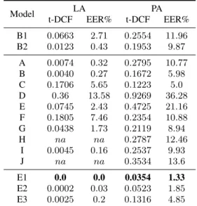
Table 1 presents the results on the original development set for both LA and PA tasks. In general, the results suggest that PA task is harder than LA. For the PA task, our CNN performs no-ticeably better when operating on the last 4 seconds of audio (model B) instead of the first 4 seconds (model A), suggesting the presence of discriminative cues at the end of each audio sig-nal which we confirm in Section 5. Furthermore, we observe a poor performance for models D and E. Apart from having to learn features directly from the raw audio, another reason could be that they involve zero-padding all signals or using a randomly selected audio segment for prediction, respectively, and thus might not be able to exploit such cues at the end of audio signals.
Table 1:Results on the LA and PA development set. Bold: best performance, na: not applicable.
Model LA PA t-DCF EER% t-DCF EER% B1 0.0663 2.71 0.2554 11.96 B2 0.0123 0.43 0.1953 9.87 A 0.0074 0.32 0.2795 10.77 B 0.0040 0.27 0.1672 5.98 C 0.1706 5.65 0.1223 5.0 D 0.36 13.58 0.9269 36.28 E 0.0745 2.43 0.4725 21.16 F 0.1805 7.46 0.2354 10.88 G 0.0438 1.73 0.2119 8.94 H na na 0.2787 12.46 I 0.0045 0.16 0.2537 9.93 J na na 0.3534 13.6 E1 0.0 0.0 0.0354 1.33 E2 0.0002 0.03 0.0523 1.85 E3 0.0025 0.2 0.1316 4.85
Table 2: Results on the LA and PA evaluation set. Bold, na: same as in Table 1. Model LA PA t-DCF EER% t-DCF EER% B1 0.2116 8.09 0.3017 13.54 B2 0.2366 9.57 0.2454 11.04 A 0.1790 7.66 na na B na na 0.1577 5.75 E1 0.0755 2.64 0.1492 6.11 E2 0.2136 9.57 0.2913 14.12 E3 0.2952 10.63 0.1465 5.43
Our i-vector feature fusion approach (model I) shows im-pressive performance on the LA task but relatively poor perfor-mance on the PA task. One reason for this could be that the i-vectors extracted using hand-crafted features are not able to cap-ture characteristics of unseen replay attack conditions. On both the LA and PA tasks, model G (IMFCC) outperforms model F (MFCC), suggesting that a focus on higher frequency informa-tion is beneficial as it might not be perfectly generated by the TTS and VC algorithms. Likewise, on the PA task, the playback device properties may impact high-frequency content. Finally, the poor performance of models H and J suggest that SCMC and LTAS features are not suitable for this task.
As expected, our ensemble model appears to benefit from combining different models for both tasks, as indicated by the strong reduction in t-DCF and EER compared to all individual models. On both tasks, E1 performs better than E2 which in turn performs better than E3.
4.2.2. Evaluation set
Table 2 shows the results on the evaluation set4. On the LA
task, model E1 has an EER of2.64% and a t-DCF of0.0755, outperforming the baselines by a large margin and securing the third rank in the ASVspoof 2019 challenge. The superior per-formance of E1 over E2 and E3 suggests that fusing multiple
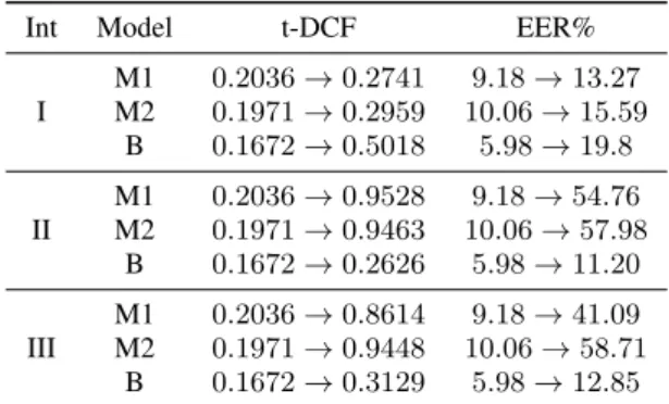
Table 3:Intervention (Int) results on the development set ofPA tasks. Numbers to the left of arrow indicates performance with-out any intervention.
Int Model t-DCF EER%
I M1 0.2036→0.2741 9.18→13.27 M2 0.1971→0.2959 10.06→15.59 B 0.1672→0.5018 5.98→19.8 II M1 0.2036→0.9528 9.18→54.76 M2 0.1971→0.9463 10.06→57.98 B 0.1672→0.2626 5.98→11.20 III M1 0.2036→0.8614 9.18→41.09 M2 0.1971→0.9448 10.06→58.71 B 0.1672→0.3129 5.98→12.85
models employing different features does provide complemen-tary information useful for spoofing detection.
However, on the PA tasks our single model B outperforms ensemble models E1 (on the EER) and E2 (both metrics). Fur-thermore, our two model ensemble E2 (A+B) outperforms the five deep model ensemble E2 and nine model ensemble E1 reaching the lowest t-DCF of 0.1465and an EER of5.43%. While these results suggest good model generalisation, it raises questions about the relevance of the cues used by model B as it is only trained on the last 4 seconds of each recording. Besides the poor performance of models D and E, the inferior perfor-mance of ensemble models on the evaluation set compared to the development set (Table 1) could be explained by model C making random predictions on the evaluation data (due to a bug we found after the challenge submission), but not on the de-velopment set – which is corroborated by the fact that model C receives the second highest weight by logistic regression in both E1 and E2.
5. Interventions on the PA task
In Table 1 we find that for the PA task, the same CNN performs much better when trained on the last4seconds of audio (model B) than on the first4seconds (model A). We thus analyse a set of audio recordings for the PA task that were confidently classi-fied by model B and find that spoofed audio tend to have more silence (zero-valued samples) at the end than bonafide exam-ples. In comparison, silence at the beginning of the recordings is often shorter and does not appear to follow this pattern. There-fore, we hypothesize that any model (deep or shallow) trained on the PA dataset that does not specifically discard this infor-mation could exploit the duration of silence as a discriminative cue. This leads to countermeasure models that are easily manip-ulated, simply by removing silence from the spoofed signals to make the model misclassify them as a bonafide signal, and vice versa. To demonstrate this effect in practice, we perform three interventions on model B and the adapted5 baselines M1 and M2 by manipulating the silence at the end of the audio signal.5.1. Intervention I
In this intervention we train the models on the original record-ings with the silence but remove them during testing6. In
Ta-5We use128mixtures to train the LFCC (M1) and CQCC (M2)
GMMs in contrast to512mixtures used in the baselines B1 and B2.
6We use a naive approach of counting the first consecutive zeros as
silence and remove them.
ble 3, a strong increase can be noticed in both EER and t-DCF for all models, suggesting that they indeed rely on the silence parts for prediction. We find that model B is most sensitive to this intervention, with t-DCF and EER rising by0.3346and an absolute13.82%, respectively. This could be due to deep mod-els focusing more strongly on silences than the GMM modmod-els, which are trained on individual spectral frames and aggregate the score through averaging frame-wise likelihoods.
5.2. Intervention II
Here, we train the model with silence parts removed, but test on the original test recordings (with silence). The stable per-formance of the CNN (model B) over the GMMs in Table 3 suggests that the former is more robust against variations in si-lence duration. On the other hand, we find a dramatic increase in error rates for M1 and M2. One interpretation for this is that bonafide and spoof GMM may assign a low likelihood to si-lence frames as they have not seen them during training. Thus, silence frames do not make large contributions to the final score making the task much harder.
5.3. Intervention III
In this intervention, we remove silence during training and test-ing to ensure that the audio samples do not share an easily ex-ploitable cue. This forces the models to learn about the actually relevant factors of interest and thus provides more realistic per-formance estimates (Table 3). As in intervention II, model B shows a stable performance indicating good generalisation and discrimination capabilities. Models M1 and M2 on the other hand achieve a poor performance, possibly since their bonafide GMM models assign a high likelihood to spoofed frames as they are very similar to bonafide ones when only considering the speech frames.
6. Discussion and conclusion
In this paper, we approach the logical access (TTS and VC) and physical access (replay) spoofing detection problem on the ASVspoof 2019 dataset using ensemble models, demonstrating that combining models trained on different feature representa-tions can be effective in detecting unseen spoofing attacks. We achieve good performance on the PA and3rd ranking on the LA tasks of the challenge. The PA task seems generally more difficult and should thus be the primary focus of future work.
Our intervention experiments in Section 5 suggests that many models trained on the PA dataset can become somewhat of a “horse”, where solving the actual problem is unintention-ally avoided by exploiting silence as trivial cues. As the evalua-tion set also contains such silences, the reported performance metrics in this task currently overestimate the actual perfor-mance. In addition to removing silence from the end of record-ings, we also removed it from the beginning, but found that it has much less impact on performance and therefore do not re-port the results in this paper. However, due to our simple ap-proach at silence removal, near-silent segments and silences be-tween words within the recording might remain and could also serve as an undesirable discriminative cue and so should be in-vestigated in future work.
We aim to perform further analysis on our deep models once the test set labels are released to the public, including the impact of the faulty deep model that produced random predic-tions on the evaluation set.
7. References
[1] D. A. Reynolds, “Speaker identification and verification us-ing gaussian mixture speaker models,”Speech Communication, vol. 17, no. 1, pp. 91–108, 1995.
[2] Z. Wu and H. Li, “Voice conversion and spoofing attack on speaker verification systems,” inAPSIPA. IEEE, 2013, pp. 1– 9.
[3] Z. Wu, N. Evans, T. Kinnunen, J. Yamagishi, F. Alegre, and H. Li, “Spoofing and countermeasures for speaker verification: A sur-vey,”Speech Communication, vol. 66, pp. 130 – 153, 2015. [4] ISO/IEC 30107-1:2016, “Information technology - Biometric
presentation attack detection - part 1: Framework,” 2016. [Online]. Available: https://www.iso.org/obp/ui/#iso:std:iso-iec: 30107:-1:ed-1:v1:en.
[5] Y. W. Lau, M. Wagner, and D. Tran, “Vulnerability of speaker verification to voice mimicking,” inProceedings of 2004 Inter-national Symposium on Intelligent Multimedia, Video and Speech Processing, 2004, pp. 145–148.
[6] Z. Wu, S. Gao, E. S. Cling, and H. Li, “A study on replay attack and anti-spoofing for text-dependent speaker verification,” in Sig-nal and Information Processing Association Annual Summit and Conference (APSIPA), 2014 Asia-Pacific, pp. 1–5.
[7] M. Todisco, X. Wang, V. Vestman, M. Sahidullah, H. Delgado, A. Nautsh, J. Yamagishi, N. Evans, T. Kinnunen, and K. A. Lee, “ASVspoof 2019: Future Horizons in Spoofed and Fake Audio Detection,” inProc. Interspeech, 2019.
[8] Z. Wu, T. Kinnunen, N. Evans, J. Yamagishi, C. Hanilci, M. Sahidullah, and A. Sizov, “ASVspoof 2015: the First Auto-matic Speaker Verification Spoofing and Countermeasures Chal-lenge,” inProc. Interspeech, 2015.
[9] T. Kinnunen, M. Sahidullah, H. Delgado, M. Todisco, N. Evans, J. Yamagishi, and K. A. Lee, “The ASVspoof 2017 challenge: Assessing the limits of audio replay attack detection in the wild,” inProc. Interspeech, 2017.
[10] ASVspoof 2019: the Automatic Speaker Verification Spoofing and Countermeasures Challenge Evaluation Plan. [Online]. Available: http://www.asvspoof.org/asvspoof2019/ asvspoof2019 evaluation plan.pdf
[11] T. B. Patel and H. A. Patil, “Combining evidences from mel cep-stral, cochlear filter cepstral and instantaneous frequency features for detection of natural vs. spoofed speech,” inProc. Interspeech, 2015.
[12] S. Novoselov, A. Kozlov, G. Lavrentyeva, K. Simonchik, and V. Shchemelinin, “STC Anti-spoofing Systems for the ASVspoof 2015 Challenge,” in 2016 IEEE International Conference on Acoustics, Speech and Signal Processing (ICASSP), 2016, pp. 5475–5479.
[13] G. Lavrentyeva, S. Novoselov, E. Malykh, A. Kozlov, K. Oleg, and V. Shchemelinin, “Audio replay attack detection with deep learning frameworks,” inProc. Interspeech, 2017, pp. 82–86. [14] P. Nagarsheth, E. Khoury, K. Patil, and M. Garland, “Replay
at-tack detection using DNN for channel discrimination,”Proc. In-terspeech, pp. 97–101, 2017.
[15] Z. Ji, Z.-Y. Li, P. Li, M. An, S. Gao, D. Wu, and F. Zhao, “Ensem-ble learning for countermeasure of audio replay spoofing attack in asvspoof2017,” inProc. Interspeech, 2017, pp. 87–91.
[16] Z. Chen, Z. Xie, W. Zhang, and X. Xu, “Resnet and model fusion for automatic spoofing detection,” inProc. Interspeech, 2017, pp. 102–106.
[17] B. L. Sturm, “A simple method to determine if a music informa-tion retrieval system is a “horse”,”IEEE Transactions on Multi-media, vol. 16, no. 6, pp. 1636–1644, 2014.
[18] B. Chettri and B. L. Sturm, “A Deeper Look at Gaussian Mix-ture Model Based Anti-Spoofing Systems,” in2018 IEEE Inter-national Conference on Acoustics, Speech and Signal Processing (ICASSP), pp. 5159–5163.
[19] B. Chettri, S. Mishra, B. L. Sturm, and E. Benetos, “Analysing the predictions of a cnn-based replay spoofing detection system,” in2018 IEEE Spoken Language Technology Workshop (SLT), pp. 92–97.
[20] V. Morfi and D. Stowell, “Deep learning for audio event detection and tagging on low-resource datasets,” Applied Sciences, vol. 8, no. 8, p. 1397, 2018. [Online]. Available: http://dx.doi.org/10.3390/app8081397
[21] J. Leeet al., “Sample-level deep convolutional neural networks for music auto-tagging using raw waveforms,” in14th Interna-tional Conference on Sound and Music Computing (SMC), 2017. [22] T. Kim, J. Lee, and J. Nam, “Sample-level cnn architectures for music auto-tagging using raw waveforms,” in2018 IEEE Inter-national Conference on Acoustics, Speech and Signal Processing (ICASSP).
[23] K. Heet al., “Deep residual learning for image recognition,” in
Proceedings of the IEEE conference on computer vision and pat-tern recognition, 2016.
[24] J. Hu, L. Shen, and G. Sun, “Squeeze-and-excitation networks,” inProceedings of the IEEE conference on computer vision and pattern recognition, 2018.
[25] D. Stoller, S. Ewert, and S. Dixon, “Wave-U-Net: A multi-scale neural network for end-to-end source separation,” inProceedings of the International Society for Music Information Retrieval Con-ference (ISMIR), vol. 19, 2018, pp. 334–340.
[26] J. Salamon, J. P. Bello, A. Farnsworth, and S. Kelling, “Fus-ing shallow and deep learn“Fus-ing for bioacoustic bird species clas-sification,” in2017 IEEE International Conference on Acoustics, Speech and Signal Processing (ICASSP), 2017, pp. 141–145. [27] S. Davis and P. Mermelstein, “Comparison of parametric
repre-sentations for monosyllabic word recognition in continuously spo-ken sentences,”IEEE Transactions on Acoustics, Speech, and Sig-nal Processing, vol. 28, no. 4, pp. 357–366, Aug 1980.
[28] S. Chakroborty et al., “Improved closed set text-independent speaker identification by combining mfcc with evidence from flipped filter banks,”IJSP, vol. 4, no. 2, pp. 114–122, 2007. [29] J. M. K. Kua, T. Thiruvaran, M. Nosratighods, E. Ambikairajah,
and J. Epps, “Investigation of spectral centroid magnitude and fre-quency for speaker recognition,” inProc. Odyssey Speaker and Language Recognition Workshop, 2010, pp. 34–39.
[30] M. Sahidullah, T. Kinnunen, and C. Hanilc¸i, “A comparison of features for synthetic speech detection,” in Proc. Interspeech, 2015.
[31] H. Muckenhirn, P. Korshunov, M. Magimai-Doss, and S. Marcel, “Long-term spectral statistics for voice presentation attack detec-tion,”IEEE/ACM Transactions on Audio, Speech, and Language Processing, vol. 25, no. 11, pp. 2098–2111, 2017.
[32] B. Chettri, B. L. Sturm, and E. Benetos, “Analysing replay spoof-ing countermeasure performance under varied conditions,” in
2018 IEEE International Workshop on Machine Learning for Sig-nal Processing (MLSP).
[33] M. Todisco, H. Delgado, and N. W. D. Evans, “A New Feature for Automatic Speaker Verification Anti-Spoofing: Constant Q Cepstral Coefficients,” inOdyssey, 2016.
[34] F. Pedregosaet al., “Scikit-learn: Machine learning in Python,”
Journal of Machine Learning Research, vol. 12, pp. 2825–2830, 2011.
[35] S. O. Sadjadiet al., “MSR Identity Toolbox v1.0: A matlab tool-box for speaker recognition research,”Speech and Language Pro-cessing Technical Committee Newsletter, 2013.
[36] N. Br¨ummer and E. D. Villiers, “The bosaris toolkit: Theory, algorithms and code for surviving the new dcf,”arXiv preprint arXiv:1304.2865, 2013.
[37] T. Kinnunen, K. Lee, H. Delgado, N. Evans, M. Todisco, M. Sahidullah, J. Yamagishi, D.A, and Reynolds, “t-DCF: a Detection Cost Function for the Tandem Assessment of Spoof-ing Countermeasures and Automatic Speaker Verification,” in