single-channel blind audio source
separation
Tobias Stokes
Submitted for the Degree of Doctor of Philosophy
Institute of Sound Recording Faculty of Arts and Human Sciences
This thesis and the work to which it refers are the results of my own efforts. Any ideas, data, images, or text resulting from the work of others (whether published or unpublished) are fully identified as such within the work and attributed to their originator in the text, bibliography, or in footnotes. This thesis has not been submitted in whole or in part for any other academic degree or professional qualification. I agree that the University has the right to submit my work to the plagiarism detection service TurnitinUK for originality checks. Whether or not drafts have been so-assessed, the University reserves the right to require an electronic version of the final document (as submitted) for assessment as above.
Given a mixture of audio sources, a blind audio source separation (BASS) tool is required to extract audio relating to one specific source whilst attenuating that related to all others. This thesis answers the question “How can the perceptual quality of BASS be improved for broadcasting applications?”
The most common source separation scenario, particularly in the field of broadcasting, is single channel, and this is particularly challenging as a limited set of cues are available. Broadcasting also requires that a source separator is automated, capable of handling non-stationary, reverberant mixtures and able to separate an unknown number of sources. In the single-channel case, the time-frequency mask is common as a method of separation. However, this process produces artefacts in the separated audio.
The perceptual evaluation for audio source separation (PEASS) toolkit represents an efficient way to generate a multi-dimensional measure of perceptual quality. Initial experimental work, using ideal target and interferer estimates, uses PEASS to test variations on the ideal binary mask and shows continuous masks are perceptually better than binary while identifying a trade-off between artefacts and interferer suppression.
To explore the optimisation of this trade-off, a series of sigmoidal functions are used to map target-to-mixture ratios to mask coefficients. This leads to a mask, with less target-to-mixture based discrimination than those typically found in literature, being identified as the optimum. Further experiments applying offsets, hysteresis, smoothing and frequency-dependency to the mask do not show any benefit in audio quality.
The optimal sigmoidal mask is demonstrated to also be superior under non-ideal conditions using a non-negative matrix factorisation algorithm to produce the estimates. A final listening test compares the outputs of binary, ratio and optimal
My foremost thanks belong with my supervisors: Tim Brookes and Chris Hummersone. They have both played a vital role throughout the completion of this project and the preparation of my thesis. I am immensely grateful for their time, wisdom and guidance.
The input of the BBC into this work has made it so much more than an academic research project. I’m particularly grateful to Andrew Mason for his supervision of the industrial side of this work. Early on, conversations with Chris Baume and Dave Marston played an important part in shaping the direction of this research. Further thanks belong with the many BBC sound supervisors and studio managers who either allowed me to observe their work or took time out of their busy schedules to discuss my work and listen to some of the audio produced.
Before commencing my PhD, I was warned that the existence of a PhD student can be incredibly lonely. However, I have been fortunate to be a part of an incredible cohort of PhD students during my time in the Institute of Sound Recording. My thanks to: Andy Pearce, Cleo Pike, Daisuke Koya, Jon Francombe, Khan Baykaner, Kirsten Hermes, Marek Olik, Phil Coleman and Tommy Ashby.
Finally, I’d like to thank my wife, Rhiannon, for her love, encouragement, patience and belief in me throughout this process.
The work in this thesis was supported by funding from the Engineering & Physical Sciences Research Council (EPSRC) and the British Broadcasting Corporation Research & Development Department (BBC R&D) by way of an Industrial Cooperative Award in Science & Technology (iCASE).
List of figures vii
List of tables ix
List of equations x
Publications arising from this thesis xiii
Chapter 1: Introduction 1
1.1 What is blind audio source separation? . . . 2
1.2 What is time-frequency masking? . . . 2
1.3 Applications of blind audio source separation . . . 3
1.4 Thesis aim . . . 3
1.5 Thesis structure . . . 4
Chapter 2: Blind audio source separation 7 2.1 Classification of BASS problems . . . 7
2.1.1 Classification of the mixtures to be separated . . . 8
2.1.2 Classification of un-mixing tasks . . . 12
2.1.3 Summary . . . 15
2.2 Methods for BASS . . . 16
2.2.1 Computational auditory scene analysis . . . 16
2.2.2 Independent component analysis . . . 31
2.2.3 Non-negative matrix factorisation . . . 36
2.2.4 Discussion . . . 39
2.2.5 Summary . . . 42
2.3 Chapter summary . . . 44 Chapter 3: Evaluating audio source separation 45
3.1.3 Vincent et al.’s method . . . 47
3.2 Subjective assessment of separation quality . . . 51
3.2.1 Stubbs & Summerfield’s test . . . 51
3.2.2 Kornycky et al.’s test . . . 51
3.2.3 Emiya et al.’s test . . . 52
3.3 Objective modelling of subjective metrics . . . 52
3.3.1 PEMO-Q . . . 53
3.3.2 The PEASS system . . . 56
3.4 Discussion . . . 58
3.5 Chapter summary . . . 59
Chapter 4: The requirements of the broadcasting industry 61 4.1 The observations . . . 62 4.1.1 Live broadcasting . . . 62 4.1.2 Event recording . . . 63 4.1.3 Programme editing . . . 65 4.2 Noise control . . . 65 4.2.1 Intellimix . . . 66
4.2.2 Dialogue noise suppressor . . . 66
4.3 Implications for an un-mixing tool . . . 67
4.3.1 The interface with the engineer . . . 67
4.3.2 Inputs and outputs . . . 67
4.4 Opinions of the sound supervisors . . . 68
4.4.1 Data compression . . . 68
4.4.2 The art of mixing . . . 69
4.5 Chapter summary . . . 69
Chapter 5: Developing source separation for the broadcasting industry 71 5.1 The TF mask for broadcasting . . . 72
5.1.1 The case for the TF mask . . . 72
5.1.2 The binary mask . . . 73
5.2.1 Representation . . . 76
5.2.2 Feature extraction . . . 76
5.2.3 Masking . . . 77
5.3 How can the binary mask be improved? . . . 78
5.3.1 Alternatives to the binary switching function . . . 78
5.3.2 Smoothing of the binary mask . . . 80
5.4 Chapter summary . . . 81
Chapter 6: Perceptual quality improvement of time-frequency masks 82 6.1 Method . . . 83
6.1.1 Audio material . . . 83
6.1.2 PEASS . . . 84
6.2 The experimental masks . . . 85
6.2.1 TF representation . . . 85
6.2.2 The ideal binary mask . . . 87
6.2.3 The dithered binary mask . . . 87
6.2.4 The noisy binary mask . . . 88
6.2.5 The cepstrally-smoothed binary mask . . . 89
6.2.6 The segmented binary mask . . . 95
6.3 Comparison . . . 95
6.3.1 Discussion . . . 95
6.4 Chapter summary . . . 97
Chapter 7: Ideal sigmoidal masking 99 7.1 Background . . . 100
7.2 Method . . . 101
7.2.1 Audio mixtures and overlap calculation . . . 102
7.2.2 Estimates . . . 103
7.3 Results . . . 104
7.4 Resolution . . . 107
7.5 Chapter summary . . . 108
Chapter 8: Non-ideal sigmoidal masking 110 8.1 Gao & Woo’s algorithm . . . 111
8.2 Experimental procedure . . . 112
8.3 Results . . . 113
8.3.1 PEASS results . . . 113
8.3.2 BSS Eval results . . . 115
8.4 Chapter summary . . . 115
Chapter 9: Optimised sigmoidal masking 116 9.1 Offset sigmoidal masking . . . 117
9.1.1 Method . . . 117 9.1.2 Results . . . 118 9.1.3 Discussion . . . 119 9.2 Hysteresis . . . 119 9.2.1 Results . . . 121 9.2.2 Discussion . . . 121 9.3 Smoothing . . . 121 9.3.1 Method . . . 123 9.3.2 Results . . . 123 9.3.3 Discussion . . . 123
9.4 Frequency dependent masking . . . 125
9.4.1 Results . . . 125
9.4.2 Discussion . . . 127
9.5 Chapter summary . . . 127
Chapter 10: Subjective assessment of separated audio quality 129 10.1 Method . . . 130
10.1.1 Assessors . . . 130
10.1.2 Test environment and set up . . . 130
10.2.1 Post-screening of assessors . . . 135
10.2.2 Data pre-processing . . . 138
10.2.3 Initial analysis . . . 138
10.2.4 Model creation . . . 142
10.2.5 Post hoc tests . . . 143
10.3 Paired comparison test . . . 145
10.3.1 Method . . . 145
10.3.2 Results . . . 146
10.4 Discussion . . . 146
10.5 Chapter summary . . . 149
Chapter 11: Conclusions and further work 150 11.1 Thesis summary . . . 150 11.1.1 Main aim . . . 150 11.1.2 Chapter 1 . . . 151 11.1.3 Chapter 2 . . . 151 11.1.4 Chapter 3 . . . 152 11.1.5 Chapter 4 . . . 152 11.1.6 Chapter 5 . . . 153 11.1.7 Chapter 6 . . . 153 11.1.8 Chapter 7 . . . 153 11.1.9 Chapter 8 . . . 153 11.1.10 Chapter 9 . . . 154 11.1.11 Chapter 10 . . . 154 11.2 Contributions to knowledge . . . 154
11.2.1 The sigmoidal continuum between the flat and binary masks 155 11.2.2 Sigmoidal optimisation of artefact-interferer trade-off . . . . 155
11.2.3 Perceptual preference for ratio mask over a binary mask . . 155
11.2.4 Negative findings . . . 155
11.3.2 An improved perceptual model . . . 156 11.3.3 The optimal TF basis . . . 157 11.3.4 Sample level mask smoothing . . . 157
List of acronyms 158
List of symbols 161
1.1 Thesis question structure . . . 6
2.1 A mixture of two sound sources being recorded at one microphone . 10 2.2 A mixture of two sound sources being recorded at one microphone in a reverberant environment . . . 11
2.3 The spectrogram of a viola playing the note A3 . . . 18
2.4 The time domain waveform of the viola playing A3 . . . 19
2.5 The spectrum of a viola playing the note A3 . . . 20
2.6 The histogram produced by a pattern matching algorithm . . . 21
2.7 The ACF of the viola playing A3 . . . 22
2.8 The SACF of a bank of 128 gammatone filters . . . 24
2.9 The absolute analytic signal of an amplitude modulated sine wave . 25 2.10 Gaussian smoothing for onset and offset detection in drum music . 26 2.11 Cross correlation to detect the ITD . . . 28
2.12 Plots of the Laplacian and Gaussian distributions both with zero mean and unity standard deviation. . . 32
2.13 Plot of entropy approximations . . . 35
2.14 The bases and coding matrices produced by an NMF algorithm . . 37
2.15 Overview of an NMF algorithm that separates spatial information . 39 3.1 A block diagram of the PEMO-Q system . . . 54
3.2 A block diagram of the PEASS system . . . 57
5.1 Overview of a typical under-determined BASS system. A TF representation is calculated before the target and interferer are estimated. Based on these estimates, the mixture is masked allowing the target estimate to be resynthesised. . . 75
6.2 Optimisation of the dithered binary mask . . . 88
6.3 Optimisation of the noisy binary mask . . . 90
6.4 CBM optimisations . . . 92
6.5 CBM optimisations . . . 93
6.6 CBM optimisations . . . 94
6.7 Results of the initial experiment . . . 96
7.1 Sigmoidal switching functions spaced on powers of two scale . . . . 101
7.2 Perceptual results for ideal sigmoidal masking . . . 104
7.3 Physical results for ideal sigmoidal masking . . . 105
7.4 Analysis of the relationship between peak OPS and TF overlap . . . 106
7.5 OPS scores for sigmoids using different TF resolutions . . . 109
8.1 PEASS results for sigmoidal masking using Gao & Woo’s algorithm 113 8.2 Physical metrics for non-ideal sigmoidal masking . . . 114
9.1 Offset sigmoidal curves . . . 118
9.2 The effect of adding hysteresis to a sigmoidal mask . . . 122
9.3 The results of the smoothing experiment . . . 124
9.4 OPS results calculated using frequency-dependent sigmoidal masking126 10.1 The MUSHRA testing interface . . . 132
10.2 eGauge analysis of assessor reliability . . . 136
10.3 eGauge analysis of assessor discrimination . . . 137
10.4 Box plots for each programme items . . . 139
10.5 Histograms of normalised assessor responses . . . 141
10.6 Bootstrapped confidence intervals for ratings of each TF mask . . . 142
10.7 The UI from the AB test . . . 146
2.1 A summary of the mixing matrix properties that classify the nature of a mixture. . . 9 2.2 The various classes of BASS tasks and their end goals . . . 13 2.3 Summary of CASA’s extraction of spectral, spatial and temporal
features. . . 29 2.4 A comparison of the processing of spectral, temporal, spatial and
statistical data by the ICA, NMF and CASA approaches. . . 41 2.5 The number of mixtures required to separate audio using different
BASS methods. . . 43 3.1 A comparison of BASS evaluation techniques. . . 60 5.1 Perceptual quality results for the TF mask from Araki et al. (2012) 75 9.1 The results of the offset sigmoidal experiment . . . 119 10.1 The programme items to be used for the listening test, their
measured overlap and the optimal OPS scores observed when separating each mixture in Chapter 7. . . 133 10.2 Mauchly’s test output table from the R console. The output shows
significant violations of sphericity for the mask and programme factors.143 10.3 The output of the analysis of variance (ANOVA) process showing
significant effects for the mask, programme and the interaction between them. . . 143 10.4 Results of the Bonferroni post hoc tests conducted between each
pairing of mask and programme item . . . 144 10.5 Showing significant differences between the ratings given to audio
from each of the masks. . . 145 10.6 Rank order comparisons of the three masks using four metrics:
1.1 The general form of an un-mixing problem . . . 2
2.1 Jutten & Hérault’s (1988) model of the un-mixing problem . . . 8
2.2 Delayed mixing . . . 11
2.3 Convolutive mixing model . . . 11
2.4 The auto-correlation function . . . 22
2.5 The first derivative of the Gaussian Function . . . 25
2.6 The cross-correlation for ITD detection. . . 27
2.7 ITD at different frequencies. . . 28
2.8 Calculation of the IID . . . 28
2.9 Calculation of kurtosis using moments . . . 32
2.10 Calculation of entropy from PDF . . . 33
2.11 Negentropy in terms of entropy . . . 33
2.12 Generalised negentropy approximation . . . 34
2.13 Hyvärinen’s first negentropy approximation . . . 34
2.14 Hyvärinen’s second negentropy approximation . . . 34
2.17 Maximum a posteriori expression of ICA in TF domain. . . 36
2.18 The first NMF update rule for the bases matrix W . . . 38
2.19 The second NMF update rule for the bases matrix W . . . 38
2.20 The NMF update rule for the bases matrix H . . . 38
3.1 Schobben et al.’s distortion calculation . . . 46
3.2 Schobben et al.’s separation quality calculation . . . 46
3.3 The ideal binary mask ratio (IBMR) . . . 47
3.6 Vincent et al.’s decomposition of a separation into error terms . . . 47
3.7 The general form of an orthogonal projector . . . 48
3.8 Vincent et al.’s calculation of the target source in an estimate . . . 48
3.9 Vincent et al.’s calculation of interference in an estimate . . . 48
3.10 Vincent et al.’s calculation of error due to noise in an estimate . . . 48 3.11 Vincent et al.’s calculation of error due to artefacts in an estimate . 48
3.12 Calculation of error due to interference . . . 49
3.13 Calculation of error due to noise . . . 49
3.14 Vincent et al.’s simplified calculation of error due to noise in an estimate . . . 49
3.15 Calculation of source to distortion ratio . . . 50
3.16 Calculation of source to interferer ratio . . . 50
3.17 Calculation of sources to noise ratio . . . 50
3.18 Calculation of sources to artefact ratio . . . 50
3.19 Calculation of the ISR . . . 50
3.20 The PEMO-Q assimilation . . . 55
3.21 The cross-correlation coefficient . . . 55
3.22 PEMO-Q’s measure of the overall error . . . 56
3.23 PEMO-Q’s measure of the target error . . . 56
3.24 PEMO-Q’s measure of the interference error . . . 56
3.25 PEMO-Q’s measure of the artefacts error . . . 56
3.26 The non-linear processing of the perceptual saliences . . . 56
5.1 The ideal binary mask . . . 73
6.1 The ideal binary mask . . . 87
6.2 The dithered binary mask . . . 87
6.3 The noisy binary mask . . . 89
6.4 The cepstral transform applied to the ideal binary mask (IBM). . . 90
6.5 The cepstrally-smoothed binary mask. . . 90
6.6 The inverse cepstral transform of a TF mask. . . 91
8.1 The conventional non-negative matrix factorisation model . . . 111
8.2 The 2D non-negative matrix factorisation model . . . 111
9.1 The modified optimal sigmoidal mask for offsetting . . . 117
9.2 The constraints applied to the offset sigmoidal masking functions . 117 9.3 The behaviour of a Preisach hysteron . . . 120
9.5 The 𝛽 curve used for hysteresis . . . 120 10.1 The eGauge reliability calculation for the 𝑗th subject . . . 135
10.2 The eGauge discrimination calculation for the 𝑗th subject . . . 136 10.3 The multimodality test specified in ITU-R BS.2300-0 (2014) . . . . 140
Conference papers
Stokes, T., Hummersone, C., Brookes, T. & Mason, A. (2014), Perceptual quality of audio separated using sigmoidal masks, in Proceedings of the 137th Audio
Engineering Society Convention, Los Angeles(Based on results in Chapter 7)
Stokes, T., Hummersone, C. & Brookes, T. (2013), Reducing binary masking artefacts in blind audio source separation, in Proceedings of the 134th Audio
Engineering Society Convention, Rome (Based on results in Chapter 6)
Book chapter
Hummersone, C., Stokes, T. & Brookes, T. (2014), On the ideal ratio mask as the goal of computational auditory scene analysis, in Naik, G. R. & Wang, W. (eds.) Blind Source Separation, Springer Berlin Heidelberg, pp. 349–368 (Inspired by results in Chapter 6)
Data Archive
1
Introduction
A key property of sound waves is that they are linearly superposable; two or more sounds can be united, either in the air or electronically, to become a sum of their parts (Howard & Angus 1996). This property has been exploited for centuries by composers scoring great chorales or symphonies combining the sounds of hundreds of sources. More recently, it has been used in the production of audio for electronic media, mixing together the signals from microphones on different parts of a band, or capturing ambient sound along with a presenter’s speech to give a location recording a sense of realism.
Not every combination of sounds is desirable and a recording may require elements to be removed. Currently, if a desired sound and an undesired sound noticeably coincide on single channel, that channel is no longer of use to a mixing engineer. While creating a sound mixture from individual sources is a straightforward process, extracting one or more sources for individual playback from a mixture is a much greater challenge, particularly when nothing is known about the original sources. This is because while a forward problem, in this case mixing, allows analysis of a system’s inputs and parameters to generate a specific output, unmixing involves using observations of a system’s output to predict a system’s input and parameters, and is an inverse problem with no unique solution (Tarantola 2005).
Academia has named this challenge blind audio source separation (BASS) (Vincent et al. 2006). Alternative names include: audio un-mixing, audio separation (Srinivasan & Kankanhalli 2003) and blind source separation (BSS) (Chan
et al. 1995). This thesis details research undertaken to improve BASS for the broadcasting industry. This opening chapter will introduce the themes of BASS and time-frequency (TF) masking and outline the research questions and structure of the thesis.
1.1
What is blind audio source separation?
BASS describes the problem of separating acoustic energy related to one sound source from a multi-source recording. The mixed sources can be assumed to overlap in frequency as well as time meaning that they can not be separated by a single filter. The problem is often formulated mathematically as
x(𝑡) =As(𝑡) (1.1)
where x(𝑡) represents the signal that is a mixture of the sources, s(𝑡), mixed according to the process A (Jutten & Hérault 1988). The aim is to uncover the inverse of A allowing the sources to be separated. In real world applications A
can not be calculated directly.
It is often convenient to classify a specific signal being separated as the target,
𝑠𝑗, and all other signals present, 𝑠𝑗′, as the interferer. Even in the case where
separation of all the signals is required this designation enables the separation of each target to be described. This is also referred to as the “one versus all” scenario (Vincent et al. 2003).
1.2
What is time-frequency masking?
In the context of BASS, TF masking refers to applying a weighting to each part of a spectro-temporal representation of an audio waveform (Yilmaz & Rickard 2004).
the interferer signal. Having applied the weighting to the TF representation, the TF transform is inverted returning the separated signal.
A specific case of a TF mask is the binary mask where elements are weighted either one or zero, meaning they are either entirely included or excluded from the separated signal (Wang 2005). While binary masking allows the separation of audio it can introduce unwanted artefacts to the audio. These artefacts are sometimes referred to as musical noise as it results from “isolated noise energies” at specific frequencies (Wang 2008).
1.3
Applications of blind audio source separation
BASS has many potential applications beyond academic research. The field of broadcasting will be considered in this work as the British Broadcasting Corporation (BBC) is a stakeholder in this project. Within broadcasting there are many potential applications. These include: advanced denoising tools for recordings; separation of content, mixed in legacy formats, so that it can be remixed for a modern surround format; removal of music, for which no licence is available, from a programme; and, providing the audience with a speech-background balance tool.
Away from broadcasting there are further applications available for semantic audio tools such as automated music transcription (O’Hanlon & Plumbley 2014) and speech recognition systems (Raj et al. 2010). Hearing prosthesis could also benefit from being able to identify sounds and decide how useful they are to the impaired listener (Wang 2008).
1.4
Thesis aim
This research in this thesis is framed in the context of the broadcasting industry, where the quality of audio must be good enough that it does not distract from the content of the broadcast being listened to. As future chapters will show, BASS
algorithms do not produce separated audio that is of a high enough perceptual quality for consumption by an audience. The main aim of this thesis is to answer the question: “How can the perceptual quality of BASS be improved for broadcasting applications?”
1.5
Thesis structure
To address the main aim of this thesis nine further questions are answered. These questions are enumerated in Figure 1.1. Some of the enumerated questions are further sub-divided within the chapters in which they are answered. The remainder of this thesis is structured as follows:
∙ The goal and practice of BASS need to be established in order to give this project a starting point and direction. Chapter 2 therefore establishes what BASS is and how it can be achieved (Question 1).
∙ In order to assess how successfully an algorithm has separated audio it is necessary to have a way of measuring the quality of the separation. Chapter 3 therefore determines how BASS techniques can be evaluated (Question 2).
∙ The BBC is a major stakeholder in this project and presents an opportunity for any resulting technologies to be applied. To allow the BBC’s needs to steer the project Chapter 4 establishes the BASS needs of the broadcasting industry (Question 3).
∙ Studies of literature and industrial practice presented in earlier chapters need to inform further investigation. Chapter 5 determines the subject of experimental investigation (Question 4).
∙ The quality of audio separated by binary masking needs to be improved before it can be applied in a practical system. Chapter 6 investigates whether binary masking performance can be improved (Question 5).
sigmoidal mask which gives optimum quality separated audio (Question 6).
∙ As real-world unmixing systems do not have access to known target and interferer signals, Chapter 8 identifies the sigmoidal mask which provides optimum quality under non-ideal conditions (Question 7).
∙ Further processing of the optimal sigmoidal mask may provide even greater quality improvements. Chapter 9 determines if further improvements to the sigmoidal mask are possible (Question 8).
∙ While PEASS provides a good model of perceptual audio quality, separated audio may ultimately be consumed by real listeners; their opinions are important. Chapter 10 establishes which TF mask real listeners prefer (Question 9).
∙ The work in this thesis gives a number of insights into how the perceptual quality of separated audio may be improved and also prompts further questions. Chapter 11 describes how the perceptual quality of BASS can be improved for broadcasting applications, summarises the thesis and proposes further work.
How can the perceptual quality of BASS be improved for broadcasting applications?
1. What is BASS and how can it be achieved? How are BASS problems classified?
How can sounds from different sources be separated? 2. How can BASS techniques be evaluated?
3. What are the BASS requirements of the broadcasting industry? What is the role of the sound supervisor?
How is noise controlled?
What are the implications for an un-mixing tool? What are the opinions of the sound supervisors? 4. What should be the subject of further investigation?
For broadcasting applications, which area of investigation looks most promising? What are the current problems in this area?
How might these problems be addressed? 5. Can binary masking performance be improved?
6. Which sigmoidal TF mask provides optimal separated audio quality?
2
Blind audio source separation
The opening chapter introduced this thesis’ goal: answering the question, “How can the perceptual quality of BASS be improved for broadcasting applications?”. Before discussions about the possibility of improving the quality of audio separated by BASS can begin, an understanding of the current state of the art is required. Specifically, the goal and practice of BASS need to be established to give the project a starting point and a direction. The aim of this chapter is to answer this thesis’ first question: “1. What is BASS and how can it be achieved?”. This aim will be achieved by a literature survey answering two sub-questions:
1.1 How are BASS problems classified?
1.2 How can sounds from different sources be separated?
These questions are answered in sections 2.1 and 2.2 respectively. Section 2.1 will provide a black-box understanding by describing BASS systems in terms of their inputs and outputs. Section 2.2 will explore a select group of systems in more depth by detailing how an audio mixture can be processed to reach a desired output.
2.1
Classification of BASS problems
Before attempting BASS it is necessary to define the exact nature of the problem that is to be solved. Authors define the BASS problem in different ways and with differing end goals. This section will answer the first sub-question of this chapter:
“1.1 How are BASS problems classified?”. This will be divided into two areas asking:
∙ “How are mixtures classified?” in Subsection 2.1.1; and,
∙ “How are the desired outcomes classified?” in Subsection 2.1.2.
The nature of the mixture determines how it might be separated. A mixture will contain signals produced by multiple sound sources. The assumption is made here that signals are overlapping both in time and frequency; otherwise they may be separated by splicing or filtering. Beyond this assumption the classification of the mixture is considered in three ways: the number of observations available, whether it is time variant and whether it is instantaneous or convolutive. The end result of BASS determines how successful a technique might be considered. At the minimum, a BASS technique must extract at least some information from a source which is contained in a mixture. At full scope, BASS is required to extract multiple sources from a single-channel mixture with complete attenuation of all other components.
2.1.1 Classification of the mixtures to be separated
The BASS problem is modelled in terms of sources, mixtures and a mixing process. Jutten & Hérault (1988) model the problem as
x(𝑡) =As(𝑡) (2.1)
where x(𝑡) is one or more mixtures of the signals s(𝑡) according to the mixing processA. With onlyx(𝑡)known, the system is required to determine information about Aands(𝑡). As this section classifies different un-mixing problems it defines forms for these three variables. The general form of the BASS problem given in Equation 2.1 is a basis for specific classification. This section will focus particularly on the nature of the mixing matrix A and the audio implications of its various
Property Expression Implications
Shape Number of rows, 𝑚, equal
to number of columns, 𝑛
Problem is determined;
A−1 can be calculated Stationarity A(𝑡) = A(𝑡+ 1) A is immutable. All data
can be used in its calculation.
Instantaneous or Convolutive A 2 or 3 dimensional Each mixture contains multiple copies of each source at multiple delays and amplitudes.
Table 2.1: A summary of the mixing matrix properties that classify the nature of a mixture.
convolutive. A summary of this section is provided in Table 2.1.
The shape of the mixing matrix
BASS is an inverse problem. Given the outcome of a mixing process the input of that process must be sought. The shape of the mixing matrix A determines how a solution to this problem may be sought. If the matrix, A, is square and non-singular then it has an inverse, A−1, which, if it can be calculated, can then be used to extract s from x. When the number of sources exceeds the number of mixtures the mixing matrix is not square and the problem is said to be over-complete or under-determined and no inverse of the mixing matrix exists. The implication of a square matrix for the BASS problem is that there must be exactly as many mixtures as sources. For techniques which rely on being able to find an inverse of the mixing matrix this is a significant constraint. Audio processing often takes many sources and mixes them to give a mono or stereo mixture.
Mixture stationarity
The model for BASS given by Equation 2.1 defines the mixing process, A, as time invariant. Assuming mixture stationarity assumes that throughout the recording there is no variation in the level, direction or positioning of any of the sources
Figure 2.1: A mixture of two sound sources being recorded at one microphone. 𝑡1 and 𝑡2 are the propagation times. Assuming 𝑡1 =𝑡2 ≈0 the mixture is instantaneous.
(Hyvärinen et al. 2001). Under circumstances where the audio is not constrained in this way the audio data only remain relevant to the un-mixing problem for a short window. Stationary mixtures have an advantage; all the data (often millions of samples in the case of audio) can be used to calculate the mixing matrix. In the case of an non-stationary mixture, the mixture signal must be windowed and recalculations made regularly to minimise errors due to non-stationarity. The mixture stationarity assumption is rarely valid for anything but the most synthetic of problems.
Instantaneous or convolutive
An important distinction is made between instantaneous and convolutive mixing. Under an instantaneous mixing model, sounds are recorded electronically at generation. In convolutive situations, delays are introduced between the creation of the sound and its recording at a microphone. In a reverberant environment, reflections then arrive at further delays. Pedersen et al. (2008) highlight the
Figure 2.2: A mixture of two sound sources being recorded at one microphone in a reverberant environment. This mixture is convolutive. Figure 2.1 will be instantaneous if the propagation times, 𝑡1 and 𝑡2, are equal to each other and close to zero. In the case where 𝑡1 ̸= 𝑡2 the mixture is no longer instantaneous as the mixing of the signals now contains a lag. Instead of the mixing model given in Equation 2.1, each mixture, 𝑥𝑗, is now a combination of
time shifted source signals
𝑥𝑗(𝑡) =
∑︁
𝑖
𝑎𝑖𝑗𝑠𝑖(𝑡−𝜏𝑖𝑗) (2.2)
where𝜏𝑖𝑗 represents the lag on each signal,𝑖is the source index and𝑗 is the mixture
index. Allowing each signal to arrive at a delay introduces an additional variable to each mixture: the delay on each signal, 𝜏. This becomes further complicated by the introduction of a reverberant environment. As shown in Figure 2.2, rather than each signal arriving at one delay and amplitude it arrives at many delays and amplitudes. 𝑥𝑗(𝑡) = ∑︁ 𝑖 ∑︁ 𝜏 𝑎𝑖𝑗(𝜏)𝑠𝑖(𝑡−𝜏) (2.3)
2.1.2 Classification of un-mixing tasks
As well as classifying the nature of the input, it is of interest to specify different required outputs. Different authors pursue differing goals for BASS and clarification of the end goal will be useful as a descriptor of each BASS problem and in choosing a metric with which to assess experimental work. This section classifies un-mixing tasks using a similar structure to that of Vincent et al. (2003). When comparing tasks an important initial distinction is whether or not the end result is to be listened to (Vincent et al. 2003). In this section two scenarios are listed which have listenability as a requirement: extraction and scene modification. Databasing tasks are also described; these are not required to return audio which is to be listened to. A summary is provided in Table 2.2.
Extraction of individual components
The most prevalent goal of BASS is the extraction of individual components (Vincent et al. 2003). In this context, a successful algorithm will return one audio stream for each source in the mixture. In each stream, the ratio of the target source to other signals will be maximised. Using extraction as an aim does cause problems as any imperfections in the separation may be obvious when the separated signal is played in isolation.
Noise Removal
Noise removal can be an important task in the production of high quality audio. While many tools exist to remove spectrally stationary sources, some of which are detailed in Chapter 4 of this thesis, there may be interfering background sounds which do not fit this spectral or temporal profile. Noise removal in this context can be seen as a subset of extraction as the extracted noise is generally discarded and does not need to retain listenable quality but this process must not damage
Task Separation quality required
Applications
Extraction The audio separated must be of the highest possible quality as it could be reused in any circumstance.
Complete remixing of a recording.
Scene Rebalancing The process should not damage the quality of the overall audio but light distortion of individual sources are likely to be masked in the mix.
Automated or audience controlled intelligent balancing of a mixture.
Databasing Sources must be recognisable by the
databasing process but do not need to be listened to.
Archive management. Source Classification. Music Information Retrieval
De-noising Target audio must not be damaged but sounds being removed do not need to be retained.
Next generation noise control tools capable of dealing with more than white noise sources Table 2.2: The various classes of BASS tasks and their end goals
for each signal, extracting the source to sound as if it was on its own in the room, or the algorithm may be required to also perform deconvolution and leave only direct sound in the resulting separation. Whichever decision is made, it should be made explicitly as evaluation techniques described later in this thesis will need to assess for either criterion.
Modification of an audio scene
There are many situations where BASS does not need to fully extract sources but to simply allow the scene which they are in to be modified. This could involve changing the spectral characteristics, spatial positioning or relative levels of individual sources. This would be useful in a number of cases, for example, in a mix where the speech intelligibility is decreased by background sound an increase
modification or rebalancing has been identified as a separate task by Vincent et al. (2003).
The point at which a scene modification becomes an extraction needs to be quantified for these two terms to provide a distinction. While extraction will allow complete scene rebuilding, there are a number of potential advantages to pursuing scene modification instead of the extraction approach. If an iterative extraction is attempted then it may be that iterations increasingly damage the remaining signals meaning increased distortion of signals extracted later in the process. The rebalancing approach allows artefacts of the process to be masked in the audio scene. This masking means perceived degradation due to artefacts is reduced. As well as the distortion advantages the rebalancing approach may also be a better approach for non-expert end users. While total extraction provides a tool for skilled restructuring of a soundtrack a rebalancing tool may provide an audience member with a way of altering the ratio of speech to background music in the mix they listen to at home. This can be controlled so the mix quality can not be impaired beyond what is necessary to provide improved speech intelligibility. The amount of flexibility provided by a BASS tool must be appropriately matched to the intended user. Rebalancing is advantageous over extraction when full control of the sources is not required but control over the balance of the mix is. If this tool is well designed it may be usable by audience members within defined constraints.
Databasing tasks
Some audio tasks are focused on extracting information from the audio rather than presenting it to an end listener. These tasks can be collectively referred to as databasing tasks and cover a number of possible scenarios.
Systems that aim to produce a score for a piece of music (Goto & Hayamizu 1999) are an example of a range of music information retrieval (MIR) tasks as described by Typke et al. (2005). Speaker identification as described by Sailaja et al. (2010)
being separated needs to be preserved the listenability does not. This approach does not seek to change the audio mixture in any way; the only aim is to extract information.
2.1.3 Summary
This section has answered the question “How are BASS problems classified?”. This has been done by classifying different mixtures and outcomes for BASS systems.
The simplest BASS systems are instantaneous, determined and stationary. There is no delay between sound generation and recording, for every source in the mixture there is an observation of the mixture to aid separation and the proportions of each sound in the mixture are time invariant. The reality is that systems are rarely this simple. Real world mixtures are convolutive. Reflections from the recording environment cause additional multiple delayed portions to become part of the signal. Mixing systems are also generally under-determined. Many sources are mixed to one or two channels. This stops a simple matrix inversion being sought to provide the separation. Stationarity is not normally a realistic constraint. The mix is altered by the movement of sources and changes made to electronic mixing equipment.
Classifying outcomes used four high level problems: source extraction, scene re-balancing, databasing and denoising. Source extraction is the most common goal of BASS but is also the most demanding as the resulting signal must be of good enough quality to listen to in isolation. Rebalancing still aims for audio that is listenable but the separation can be less perfect as some artefacts will be masked in the mixture. Databasing tasks focus on the significance of audio features and while not requiring perfect extraction may require more in depth identification of audio elements.
2.2
Methods for BASS
Separating audio from a mixture has been a research interest since Cherry (1953) described the “cocktail party problem”, the human listener’s ability to “recognise what one person is saying when others are speaking at the same time”. This section will answer this chapter’s second question: “1.2 How can sounds from different sources be separated?”. This section will focus on distinguishing sounds from different sources within a mixture. Four key criteria for distinguishing sources are presented: spectral similarity, temporal continuity, spatial distinction and statistical independence. These are described in the context of computational auditory scene analysis (CASA), independent component analysis (ICA) and non-negative matrix factorisation (NMF). At the end of the chapter a comparison of methods is provided in terms of the cues used for separation.
2.2.1 Computational auditory scene analysis
CASA is a technique inspired by Bregman’s (1990) work on source separation by the human auditory system. Bregman’s studies of auditory scene analysis (ASA) detail observations of the human auditory system’s ability to separate sounds from an audio scene. Wang & Brown (2006) bring together a number of key ideas in producing a computational model of ASA.
While the goal of early CASA research was to model the ASA process in humans (Brown 1992; Ellis 1996), researchers have used CASA principles for source separation. When trying to perform CASA inspired source separation, the computational goal is widely believed to be the ideal binary mask (IBM) (Wang 2005). From a TF representation of the mixture audio—which is often obtained using a gammatone filterbank (Patterson et al. 1987)—the IBM designates each TF cell with either a one or a zero depending on whether that element is primarily part of the target source’s energy or not. The processes described in this section
is calculated from a signal using three stages:
1. the audio is processed to form a perceptually-relevant TF representation; 2. spectral, temporal and spatial features are extracted and used to segment
the auditory scene; and
3. the segments are grouped by source.
This section will focus on features that can be used for separation, how they are extracted by a separation algorithm and how sounds can be subsequently separated. Spectral cues are discussed first, followed by temporal cues (page 23) and finally spatial cues (page 26). A summary is given at the end of the section on page 30.
Fundamental frequency detection
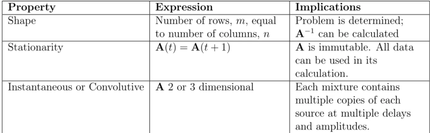
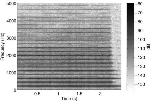
In harmonic sounds, for example pitched musical instruments or voiced speech, the frequency-spacing of the resonances is related by an integer-multiple relationship. The lowest frequency is the fundamental, 𝑓0, and all its harmonics are related by integer multiples. Figure 2.3 shows the harmonics of a note played by a viola. The detection of fundamental frequencies provides a method of grouping parts of a TF audio representation. Having established which peaks in the frequency spectrum are fundamentals, peaks at integer multiples of the fundamentals can be grouped. There are both spectral and temporal methods for 𝑓0 detection. This section details 𝑓0 detection using three approaches: spectral, temporal and spectro-temporal. Each approach is demonstrated using a monophonic example to establish its principles. Polyphonic problems are then described as an extension of the monophonic techniques. Throughout this section the example of a viola playing the note A3 (𝑓0 ≈ 220 Hz) is used. The recording is taken from the University of Iowa’s sample library of anechoic instrument recordings1. A section
of the waveform from this signal is shown in Figure 2.4, in which the periodicity of the waveform is clear.
0.5 1 1.5 2 0 1000 2000 3000 4000 5000 Time (s) Frequecy (Hz) dB −150 −140 −130 −120 −110 −100 −90 −80 −70 −60
Figure 2.3: The spectrogram of a viola playing the note A3. The harmonics are visible as lines running across the image. 𝑓0 is the lowest of the harmonics.
Spectral 𝑓0 detection There are a number of approaches to extracting the fundamental frequency from a spectrum; some are more generally applicable than others. The example spectrum shown in Figure 2.5 shows the fundamental is both the lowest and the largest peak. However this is not always the case and neither of these factors definitely indicate that a peak represents the fundamental. The fundamental can still be calculated in cases where it is entirely missing. The prevailing technique for calculation of 𝑓0 from the spectrum was first applied to speech by Schroeder (1968) and is called pattern matching. This technique involves dividing the frequency of each peak in the spectrum by an incremental series of integers and plotting the results on a histogram. Figure 2.6 shows the
0 2 4 6 8 10 12 −1 −0.5 0 0.5 1 Time (ms) Amplitude
Figure 2.4: A short segment of the time domain waveform of a viola playing the note A3.
detailed an algorithm that found the first 𝑓0 and then removed it along with all peaks harmonically related to it. The residual spectrum was then searched for a further 𝑓0 with the detect-and-remove process being iterated as many times as necessary. This technique is flawed in cases where the multiple voices are harmonically related as they will share harmonics at certain peaks. Removal of peaks belonging to more than one source will deprive the algorithm of information to find fundamentals on later iterations.
Temporal 𝑓0 detection Calculation of the fundamental frequency is also possible working in the time-domain. While techniques such as measuring the distance between peaks and counting zero-crossings work for a subset of periodic waveforms, a better estimate is obtained by the use of the auto-correlation function (ACF) (Licklider 1951). The ACF measures the correlation of a waveform, 𝑥(𝑛), to
time-500 1000 1500 2000 2500 3000 3500 4000 0 50 100 150 200 250 300 350 Frequency (Hz) Amplitude
Figure 2.5: The spectrum of a viola playing the note A3. The harmonic structure is shown by the peaks.
0 500 1000 1500 2000 0 1 2 3 4 Frequency (Hz) Count
Figure 2.6: Pattern matching performed to find a missing fundamental of 220 Hz. To produce the histogram, locations of the peaks in the spectogram: 440, 660, 880 and 1760 Hz, were each divided by the integers 1 to 10. The most frequently occuring value in the histogram is 220 Hz.
shifted versions of itself. The discrete form of the ACF is given by ACF(𝜏) = 1 𝑊 𝑛=𝑡+𝑊 ∑︁ 𝑛=𝑡+1 𝑥(𝑛)𝑥(𝑛+𝜏) (2.4)
where 𝑡 is the time index, 𝜏 the time lag and 𝑊 is the window of summation. The ACF produces peaks spaced by 𝑓1
0, the fundamental time period. The ACF of the example viola note is shown in Figure 2.7. The time-domain approach has
200 400 600 800 1000 1200 1400 1600 −3 −2 −1 0 1 2 3 4 5 6 Lag time τ ACF(y)
Figure 2.7: The ACF of the viola playing the note A3. The peaks are clearly spaced by 200 samples. This is the time period of the fundamental frequency in samples. Division of 44.1 kHz by 200 samples recovers the frequency.
been used to solve multiple𝑓0 problems. Like the spectral technique the aim is to remove the first 𝑓0 detected and then repeat the algorithm to detect the second
described previously for spectral techniques can be implemented.
Spectro-temporal𝑓0detection Inspired by Licklider’s (1951) duplex theory of pitch perception, modern CASA systems tend to use spectro-temporal methods to detect
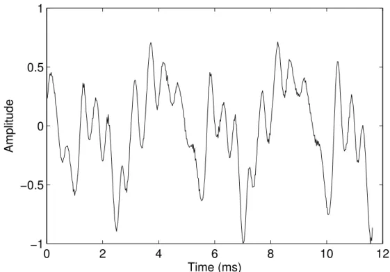
𝑓0. Licklider states, “That frequency and period are reciprocally related is not sufficient reason for throwing one away and examining only the other” and then goes on to demonstrate analysis of both within the human auditory system. To realise this in a system the original signal is passed through a filterbank and then an ACF performed on each frequency band (Wang & Brown 2006). The ACFs are then summed across all frequency bands at each lag. The resulting measure is often called the SACF. As with the single ACF approach discussed previously the distance between the peaks gives the period of the fundamental. The SACF is shown in Figure 2.8.
Envelope, onset and offset detection
There are a number of interesting temporal features of audio which can aid BASS. Detection of onset and offset and then full envelope calculation will be detailed here. Onset and offset information is useful to derive as it gives end points which should have common frequency content between them. Detection of the overall envelope of a sound may aid separation as changes in energy can easily be observed. Amplitude information helps identify temporal features of each source. The start and end point of sound events aid segmentation of the audio scene. Onsets and offsets allow the temporal characteristics of segments to be detected even when they occur in the presence of other sounds.
Envelope Calculation The envelope or amplitude modulation of the signal is a measure of how the amount of energy in a signal changes over time. A common representation of a signal’s envelope is the absolute analytic signal. This can be calculated in four fast Fourier transform (FFT) based steps as demonstrated by Hartmann (1998):
Centre Frequency (Hz) 240 510 920 1570 2570 4150 ACF −1 −0.5 0 0.5 1 100 200 300 400 500 600 0 10 20 Lag time τ SACF(y)
Figure 2.8: Top: the ACF of each output of a bank of 128 gammatone filters (using code from Jin (2007)). Bottom: The SACF taken by summing across the top plot at each lag time. The audio is the same viola sample as used previously.
1. take the FFT of the signal;
2. set the negative frequency components to zero; 3. take the inverse FFT; and
4. calculate the absolute value and multiply it by two.
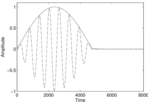
This technique will provide the absolute analytic signal as shown by the example in Figure 2.9.
0 2000 4000 6000 8000 −1 −0.5 0 0.5 1 Amplitude Time
Figure 2.9: The absolute analytic signal of an amplitude modulated sine wave. The dashed line shows the modulated sine wave.
not all be interpreted as onsets. It is common to apply smoothing by means of convolution of the signal envelope with the first derivative of a Gaussian function (Wang & Brown 2006),
𝐺′(𝑡, 𝜎) = −𝑡 𝜎3√2𝜋exp (︂ − 𝑡 2 2𝜎2 )︂ (2.5) where𝜎 is the Gaussian width. This convolution with the first derivative provides a smoothed and differentiated signal. From this point, the processed signal’s peaks and troughs above a certain threshold are identified. Peaks are taken as onsets and troughs as offsets (Wang & Brown 2006). The effect of applying this process to some djembe music shown in Figure 2.10.
−1 −0.5 0 0.5 1 Magnitude 0 2 4 6 8 10 x 104 −2 0 2 4 Magnitude Time (samples)
Figure 2.10: Gaussian smoothing of djembe music. Top: The original waveform. Bottom: The signal envelope convolved with the differentiated Gaussian function given in Equation 2.5
Analysis of spatial information
The human auditory system is binaural; we each perceive our surroundings using two ears. Binaural hearing provides the ability to determine spatial information about sound sources. Commercial audio is often produced in stereo, allowing spatial information to be conveyed and the listener to detect sound sources’ positions in recordings. Two fundamental binaural cues form the basis for analysis of spatial information: the aural intensity difference (IID) and the inter-aural time difference (ITD). The human auditory system is capable of localisation under reverberant conditions aided by the suppression of delayed signal portions
beamforming and multiple signal classification (MUSIC) (Schmidt 1986) rely on large microphone arrays to perform location based separation. In contrast, the techniques focused on here will aim to locate sources from a two-channel recording. The methods described here relate specifically to a recording made with a binaural head but similar techniques can be applied to a two-channel stereo recording. For two-channel stereo recordings created with a spaced pair of microphones there is no model of the human head between the microphones; time and level differences between the channels will be a function of the distance between the microphones and the speed and attenuation of sound in air. As a result, the time and level differences are likely to be smaller with a spaced pair of microphones than a binaural recording head.
The inter-aural time difference The ITD is the difference in time of arrival of a sound at each ear. The speed of sound in air is approximately 340 m/s and sound will arrive at each ear at different times when the source is not anywhere in the median plane of the listener. This difference allows azimuth to be calculated. When working with sine tones, it is common to refer to the inter-aural phase difference (IPD) as a time difference is a phase shift for a pure tone (Wang & Brown 2006). The ITD can be calculated using a cross-correlation of the two signals. Each filter bank channel can be cross correlated with its equivalent in the opposite ear. The cross correlation function (CCF) is calculated as
ccf(𝑛, 𝑐, 𝜏) = 𝑀−1
∑︁
𝑘=0
𝑎𝐿(𝑛−𝑘, 𝑐)𝑎𝑅(𝑛−𝑘−𝜏, 𝑐)ℎ(𝑘) (2.6)
using 𝑀 samples and a windowing function ℎ, 𝑛 and 𝑐 index the time steps and filter bank channels respectively. The use of the CCF is shown by the plots in Figure 2.11. The lag which gives the maximum cross correlation, 𝜏, can be equated to 𝜃, the azimuth using
𝜏 =
{︃
(𝑟/𝑐)2 sin𝜃 𝑓 ≤500Hz
Centre Frequency (Hz) 240 510 920 1570 2570 4150 −8 −6 −4 −2 0 2 4 6 8 x 10⁻⁵ −50 0 50 100 −50 5 10 15 x 10−4 Lag time τ SCCF
Figure 2.11: Cross correlation to detect an ITD of 453 𝜇s. Top: the CCF of each filter bank channel. Bottom: The SCCF calculated by summing the CCFs at each value of 𝜏.
where 𝑟 is the radius of the head (which is assumed to be spherical) and 𝑐 is the speed of sound (Wang & Brown 2006).
The inter-aural intensity difference The IID, sometimes also referred to as the inter-aural level difference (ILD), is caused by the head attenuating the sound reaching the far ear. The IID can be expressed in dB as
IID= 20 log(𝐿/𝑅) (2.8)
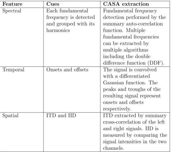
Feature Cues CASA extraction Spectral Each fundamental
frequency is detected and grouped with its harmonics
Fundamental frequency detection performed by the summary auto-correlation function. Multiple
fundamental frequencies can be extracted by multiple algorithms including the double difference function (DDF). Temporal Onsets and offsets The signal is convolved
with a differentiated Gaussian function. The peaks and troughs of the resulting signal represent onsets and offsets
respectively.
Spatial ITD and IID ITD extracted by summary cross-correlation of the left and right signals. IID is measured by comparing the signal intensities in the two channels.
Table 2.3: Summary of CASA’s extraction of spectral, spatial and temporal features.
with the work of Birchfield & Gangishetty (2005) being one of few preliminary studies.
Segmentation and grouping
Having identified key auditory features, a CASA algorithm must use the features extracted to segment the TF representation of the audio. Wang & Brown (2006) define a segment as a TF region where the “underlying acoustic energy originates primarily from the same sound source”. The segments form part of the CASA goal, the IBM, each segment is a part of the IBM for a source. To construct the
IBM for each source its segments must be grouped. Grouping is performed in two stages: simultaneous grouping and sequential grouping. Simultaneous grouping takes segments that occur simultaneously and groups them if they are part of the same source. This can be achieved using pitch tracking, for harmonic sounds, and onset and offset detection for inharmonic parts of the sound (Wang & Brown 2006).
Sequential grouping aims to group sounds from the same source across time. This is more challenging than simultaneous grouping as the characteristics of a source can change over time. Simpler algorithms perform sequential grouping using measurements of spectral similarity or pitch. Model-based grouping algorithms, such as that developed for speech by Barker et al. (2005), compare the segments with models being developed for each source and perform a maximum-likelihood estimation.
Summary
This subsection has answered the question “How does CASA separate audio?”. CASA’s separation of audio is performed by estimating the IBM. The main focus has been on feature extraction, which is necessary to perform this estimation. The key spectral feature is the fundamental frequency,𝑓0, which can be estimated using spectral, temporal or spectro-temporal techniques. Temporal features that can be extracted are the onset and offsets, or, for a more complete picture of temporal activity, the absolute analytic signal can be calculated to represent the temporal envelope. Spatial cues are extracted through calculation of time differences and intensity differences. These features are summarised in Table 2.3. Extracted features are used to group TF elements together to create a binary mask for each source in the mixture. Simultaneous grouping brings together harmonic and inharmonic segments belonging to the same source. Sequential grouping is used to group segments through time, based on the similarity of each section.
2.2.2 Independent component analysis
ICA is a technique being researched for source separation in a number of fields including BASS. Rather than looking to separate the audio in time or frequency, statistical groupings are used. To statistically separate sources, an initial assumption is required: sounds from physically independent sources will produce statistically independent signals (Stone 2004). In a mixture situation where this assumption is valid, an algorithm can then seek to separate the signals in a way that maximises their statistical independence.
ICA is a technique that seeks to separate components based on statistical independence (Jutten & Hérault 1988; Bell & Sejnowski 1995; Hyvärinen 1999). The technique aims to find the inverse mixing matrix which provides the most independent separated source signals. ICA techniques do not calculate independence directly but instead rely on simpler metrics which indicate independence.
The central limit theorem dictates that summing together independent components will lead to a variable which has a distribution that is more Gaussian than the distribution of any of the variables used to create it. From this it can be inferred that the un-mixing matrix providing the least Gaussian separated signals would most likely be the correct matrix. The rest of this section describes different measures of Gaussianity and their application in performing ICA.
There are limitations to the independence assumption: it is a poor assumption for music where multiple sources have been mixed to complement each other’s spectro-temporal content. Puigt et al. (2009) studied the independence of music and speech mixtures when measured over different excerpt sizes. Musical mixtures were shown to be highly dependent over shorter time windows. Shorter time windows are necessary when separating non-stationary mixtures.
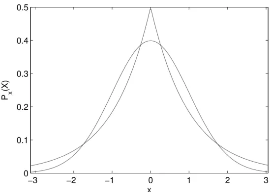
−3 −2 −1 0 1 2 3 0 0.1 0.2 0.3 0.4 0.5 x P x (X)
Figure 2.12: Plots of the Laplacian and Gaussian distributions both with zero mean and unity standard deviation.
Kurtosis
Kurtosis is a measure of how raised a distribution is at its central point in comparison with a Gaussian distribution. Figure 2.12 shows the Laplacian and Gaussian distributions and the higher kurtosis of the Laplacian is clear. The classical statistical calculation of kurtosis uses moments
𝑘(𝑥) =E{𝑥4} −3|E{𝑥2}|2 (2.9) where 𝐸{·}is the expectation of a variable.
Entropy
Entropy is a measure of the uniformity of a distribution or alternatively can be viewed as the amount of information present in a signal (Shannon 1948). A uniform distribution displays maximum entropy. The entropy of a discrete variable can be evaluated using 𝐻(𝑥) =−1 𝑁 𝑁 ∑︁ 𝑡=1 ln𝑃𝑥(𝑥𝑡), (2.10)
where𝑥is a variable with𝑁 possible values and𝑃𝑥(𝑥𝑡)is the probability that𝑥=
𝑥𝑡. Entropy is a useful feature of the signal as it can be compared with the entropy
of a Gaussian signal to determine how much more information is being given. The concept of comparing signal entropy with the entropy of a Gaussian signal is the basis for negentropy. Negentropy is defined as the difference between the entropy of a dataset and the entropy of a Gaussian distribution. This measure has two desirable characteristics: firstly, it is zero for Gaussian distributions putting the point of reference at the origin; secondly, negentropy is always non-negative. Negentropy can therefore be viewed as a robust measure of how non-Gaussian the signal is. The negentropy, 𝐽(𝑥), of a signal is defined as
𝐽(𝑥) = 𝐻(𝜐)−𝐻(𝑥), (2.11) where 𝐻(𝜐) is the entropy of a Gaussian signal with equal mean and variance to 𝑥. Negentropy is considered a more robust measure of non-Gaussianity than kurtosis. The measure provided by kurtosis is sensitive to outlying data (due to the rapid growth of the quartic term in Equation 2.9).
Approximating negentropy
Due to a lack of knowledge about the PDFs of the signals to be extracted and for computational efficiency it is necessary to approximate the entropies in Equation 2.11 to give an estimated negentropy. While Equation 2.11 gives a precise calculation of negentropy a more general difference of two functions can be taken.
With 𝐺 as any non-quadratic function negentropy can be approximated to
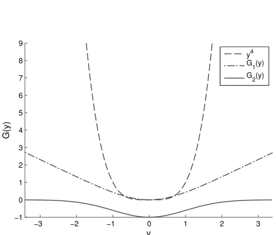
𝐽(𝑥)∝[E{𝐺(𝑥)} −E{𝐺(𝜐)}]2 (2.12) While this approximation is not always accurate, it will remain consistent with negentropy as a robust non-negative measure of how non-Gaussian a signal is. Hyvärinen (1999) suggests two functions as approximations for entropy. They are selected for their similarity in shape and less than fourth order growth characteristics. These two functions are:
𝐺1(𝑦) = 1 𝑎1
log(cosh(𝑎1𝑦)) (2.13)
𝐺2(𝑦) = −exp(−𝑦2/2) (2.14) with 1 ≤ 𝑎1 ≤ 2 but often set as one. These functions are favoured as approximations due to their similarity in shape to kurtosis. Further advantages are given by the ease with which the functions may be differentiated to obtain their gradients. A graphical representation of the negentropy approximations is shown in Figure 2.13.
Iteration
With a model for independence an un-mixing matrix must then be initialised and optimised to produce maximally independent separated signals. This optimisation is performed by use of a gradient algorithm, the most popular of which is Hyvärinen & Oja’s (1997) FastICA algorithm. The optimisation algorithm updates the un-mixing matrix so that the independence of the audio it separates is optimised towards a maximum. Assuming the independence assumption was valid, the algorithm will converge to provide an un-mixing matrix will that produce separated sources.
−3 −2 −1 0 1 2 3 −1 0 1 2 3 4 5 6 7 8 9 y G(y) y4 G1(y) G2(y)
Figure 2.13: The functions in equations 2.13 and 2.14 with the quartic term as used in kurtosis for comparison.
Extension to the TF case
Whilst it is common to explain ICA in the domain it is not purely a time-domain technique. One case of adaptation of the mixture model and cost functions to further dimensions is detailed in Naik & Kumar (2011). Redefining the sources as
𝑠=CΦ (2.15)
for coefficients Cof the TF basis Φ. The new mixture model
𝑥=ACΦ (2.16)
allows an estimate of ACto be calculated giving the weightings of the TF regions for the separated sources. These matrices are calculated using a maximum a posteriori approach expressed as
max
A,C 𝑃(A,C|𝑥)∝maxA,C 𝑃(𝑥|A,C)𝑃(C) (2.17)
2.2.3 Non-negative matrix factorisation
NMF was introduced by Lee & Seung (1999) for the learning of images by parts. The algorithm has also proved useful for BASS. The NMF approach is similar to ICA: it aims to factorise a mixture into two matrices. The constraints of NMF are different to those of ICA. The requirement for a mixture to be determined is removed and the NMF approach works with single channel audio. Extra information is gained by using a TF representation of the input signal.
NMF aims to factorise the TF representation of a mixture into two matrices, the bases, W, and the coding H. The bases matrix is formed from a set of unique spectral structures; each basis does not represent a source in the mixture but
speech into individual formants. The number of bases, usually termed 𝑟, is taken in by the algorithm as prior information. Example bases and coding matrices are shown in Figure 2.14. 0 1000 2000 3000 1 2 Frequency (Hz) Component Number W 200 400 600 1 2 H Component Number Time Window
Figure 2.14: The bases and coding matrices produced by an NMF algorithm. Two flute notes played separately and then together are shown. Their spectral information is contained in W, the left-hand matrix, while their activations are shown in H, the right-hand matrix. Produced using the NMF library available made available by Grindlay (2010).
After giving the algorithm a TF representation,V, and the number of bases,𝑟, each matrix is initialised with random non-zero values to prevent divide-by-zero errors. The algorithm then iterates update rules on W and H with the improvements in one allowing the other to be further improved. The bases or dictionary matrix
W is iterated by two update rules. The first works through time ensuring the amount of energy assigned to each frequency in each component is consistent with
activation of that component at that point in time. This is achieved by the first update equation, W𝑖𝑎 ←W𝑖𝑎 ∑︁ 𝜇 V𝑖𝜇 (WH)𝑖𝜇 H𝑎𝜇 (2.18)
where 𝑖 indexes frequency, 𝜇 indexes time steps and 𝑎 indexes bases. A ratio greater than one causes the algorithm to add energy from that frequency and less than one takes away energy. The ratio is multiplied by H for that component at that point in time. This means energy is apportioned to the component according to its level of activation at that point in time.
The second update rule for W updates the matrix to constrain each column to sum to unity. This prevents more energy being apportioned at a given frequency than was present in the original signal. This is achieved by dividing each element by the sum of its column
W𝑖𝑎 ←
W𝑖𝑎
∑︀
𝑗W𝑗𝑎
(2.19) The coding matrix H is updated by only one equation that is similar to Equation 2.18. This works through the frequency spectrum and increases the activations of components that contain more spectral energy and reduces the activation of the signals with less spectral energy. The update equation is given as, H𝑎𝜇 ←H𝑎𝜇 ∑︁ 𝑖 W𝑖𝑎 V𝑖𝜇 (WH)𝑖𝜇 (2.20) where𝑖 is used as a frequency index. For stopping conditions the algorithm either runs to a fixed number of iterations or measures the change on each update and stops when this change falls below a minimum value.
Smaragdis & Brown (2003) highlighted the issue of prior information in NMF algorithms. As this algorithm separates audio “based on the system’s accumulated experience from the presented input and not on predefined knowledge” this means that “all unique events are understood to be a new component”; simultaneous
identified the combined note as one component and the first individual note as the second. This problem can be overcome by providing the algorithm with training data. This process initialises the basis matrix with expected components rather than random values. Providing the algorithm with prior information has been shown to improve results compared to using randomly initialised matrices (Wang & Plumbley 2006).
Spatial information
The basic algorithm presented above is designed for single-channel audio and hence does not offer a method of calculation of the position of sources. An extension to the NMF algorithm presented by Parry & Essa (2006) does allow a further matrix to be added to the factorisation which details spatial positioning for a two channel mixture. This technique is built assuming spatial stationarity and may prove difficult to adapt to signals which are moved in space. The initial factorisation is demonstrated in Figure 2.15.
V
TF Representation n x m=
Spectral InformationW
n x rQ
Spatial Information r x rH
Temporal Information r x m Figure 2.15: The factorisation performed by Parry & Essa (2006). Showing the dimensions and arrangement of the spectral, spatial and temporal matrices. The algorithm’s inputs areV, the TF representation, and 𝑟 the number of sources.2.2.4 Discussion
This chapter has so far detailed different features which can be used for BASS and how they are utilised by the different techniques. This section will now briefly compare the techniques. The comparisons made in this section relate to cues and