Vol. 9 (2015) 2255–2292 ISSN: 1935-7524
DOI:10.1214/15-EJS1073
A Fisher consistent multiclass loss
function with variable margin on
positive examples
Irene Rodriguez-LujanBioCircuits Institute, University of California, San Diego, La Jolla, CA 92093-0328, USA
Machine Learning Group, Escuela Polit´ecnica Superior, Universidad Aut´onoma de Madrid,
28049 Madrid, Spain e-mail:[email protected]
and Ramon Huerta
Rady School of Management & BioCircuits Institute, University of California, San Diego,
La Jolla, CA 92093-0328, USA e-mail:[email protected]
Abstract: The concept of pointwise Fisher consistency (or classification calibration) states necessary and sufficient conditions to have Bayes consis-tency when a classifier minimizes a surrogate loss function instead of the 0-1 loss. We present a family of multiclass hinge loss functions defined by a con-tinuous control parameterλrepresenting the margin of the positive points of a given class. The parameterλallows shifting from classification uncal-ibrated to classification caluncal-ibrated loss functions. Though previous results suggest that increasing the margin of positive points has positive effects on the classification model, other approaches have failed to give increasing weight to the positive examples without losing the classification calibra-tion property. Ourλ-based loss function can give unlimited weight to the positive examples without breaking the classification calibration property. Moreover, when embedding these loss functions into the Support Vector Machine’s framework (λ-SVM), the parameterλdefines different regions for the Karush—Kuhn—Tucker conditions. A large margin on positive points also facilitates faster convergence of the Sequential Minimal Optimization algorithm, leading to lower training times than other classification cali-brated methods.λ-SVM allows easy implementation, and its practical use in different datasets not only supports our theoretical analysis, but also provides good classification performance and fast training times.
MSC 2010 subject classifications:68T10.
Keywords and phrases:Multiclass classification, classification calibra-tion, Bayes consistency, Fisher consistency, hinge loss functions, Support Vector Machine.
Received November 2014.
Contents
1 Introduction . . . 2256
2 Classification calibration for multiclass loss functions . . . 2259
3 Family of loss functions with variable margin λ . . . 2262
3.1 Connection with other multiclass loss functions . . . 2262
4 Classification calibration domain . . . 2264
5 Classification calibration for Support Vector Machines . . . 2265
6 Experimental evaluation . . . 2271
6.1 Comparison with other multiclass-SVM implementations . . . . 2275
7 Conclusions . . . 2276
A Detailed proof of Theorem2. . . 2277
Acknowledgments . . . 2288
Supplementary Material . . . 2289
References . . . 2289
1. Introduction
Many of the most used classification algorithms are based on the minimiza-tion of a surrogate convex loss funcminimiza-tion since the direct minimizaminimiza-tion of the 0-1 loss is computationally intractable. Some examples of these algorithms include Support Vector Machines (SVMs) [8,10, 34], boosting [13, 7,22], and logistic regression [14]. Conditions such as convexity, continuity, and differentiability of these surrogate loss functions are easy to analyze; however, the statistical implications of using these surrogate loss functions are not so evident [2]. The notion of classification calibration was initially defined by Bartlett et al. [2, 3] as a pointwise form of Fisher consistency for classification. It was shown to be a necessary and sufficient condition for a binary classifier to be Bayes consistent when the empirical risk Ψ of a surrogate loss function converges to the minimal possible Ψ-risk. Tewari and Bartlett [37, Theo. 2] extended this classification cal-ibration concept to multiclass problems. However, the extension of binary loss functions to multiclass classification settings is non-trivial, leading to a large body of research to better understand classification calibration in multiclass scenarios [23,26, 37,41, 42, 43,28, 40]. The main contribution of this work is the formulation of a pointwise Fisher consistent (classification calibrated) mul-ticlass loss function that can give arbitrary high weight to the margin of the positive points, which is shown to beneficial in terms of classification accuracy and training times. Our loss function overcomes some limitations of previous approaches since (i) it allows overweighting the margin of positive points while maintaining classification calibration, (ii) it yields consistent classification ac-curacies with respect to the classification calibration domain, and (iii) it can be efficiently trained when embedded in the Support Vector Machine’s framework (λ-SVM).
There exist two main strategies to extend binary learning algorithms to a multiclass setting. The first approach consists of formulating the multiclass
clas-sification problem as a combination of several binary clasclas-sification tasks. It in-cludes strategies such as one-versus-rest, one-versus-one, and pairwise coupling [1]. Though these strategies are easy to implement, having optimal solutions of those binary classifiers does not guarantee having a global optimal solution for the multiclass problem. Additionally, the multiclass loss function does not nec-essarily inherit the classification calibration properties of its binary counterpart [37, 26, 42]. For example, the hinge loss function commonly used in Support Vector Machines has shown to be classification calibrated for binary problems [25], but the one-versus-rest strategy may be inconsistent when there is no a dominating class [26]. The second approach is based on the formulation of mul-ticlass surrogate loss functions to use the same global optimization procedure as in the binary case. Though several multiclass hinge loss functions can be found in the literature [39, 9, 23, 28, 19], only two of them have been shown to be classification calibrated for every multiclass problem: Lee et al.’s loss function [23] and Liu and Yuan’s loss function1(reinforced multicategory hinge loss) [28]. However, these approaches present some limitations. On the one hand, Lee et al.’s loss function does not consider the slack of the positive points of a given class, so it overlooks valuable information for the classification algorithm as it will be shown in our experiments (Section6). On the other hand, the reinforced multicategory hinge loss considers both the margin of the positive and nega-tive points of a given class, but experimental results in [28] on two synthetic datasets show that best classification performances are obtained for values ofγ
that overweight the margin of the positive points, and make the loss function classification uncalibrated. As pointed out by the authors, this is a surprising result. However, it points out the importance of paying attention to the error of positive examples. Additionally, the reinforced multicategory hinge loss as-signs a margin of (L−1) to the positive points, with Lthe number of classes, which is justified as a natural choice to have sum-to-zero loss functions. Unfor-tunately, using this margin in the context of Support Vector Machines is not beneficial for the optimization algorithm as it represents a boundary between different Karush—Kuhn—Tucker (KKT) conditions as we show in Proposition3 (Section 5). A more detailed comparison between the different multiclass loss functions proposed in the literature can be found in Section 3.1.
The key contributions of this paper are:
• Formulation of a new family of multiclass hinge loss functions with a single control parameterλ∈Rthat represents the margin of the positive points of a given class. Our family of loss functions takes into account both the error of the positive and negative points of a given class, and it allows us to freely overweight the error associated to the positive points without losing classification calibration. A property that was attempted by Liu and Yuan [28] and Huerta et al. [19], but was not fully completed.
• Characterization of the classification calibration domain of this family of hinge loss functions. We show that its classification calibration
proper-1Liu and Yuan’s loss function is classification calibrated for certain values of a meta– parameterγ.
Fig 1. Connections between different multiclass loss functions proposed in the literature and
our family of variable margin loss functions.
ties can be fully controlled by λ. This analysis reveals that our family of loss functions is classification calibrated provided that the margin of the positive points is larger or equal than (L−2)/2 with L the number of classes in the problem. This interesting property makes it possible to define a classification calibrated hinge loss function for every multiclass classification problem while overweighting the error of positive points. In other words, as long as one choosesλ /∈[0,(L−2)/2] one can optimize the
λmeta–parameter guaranteeing the classification calibration property.
• Formulation of a common framework that allows connecting the new fam-ily of loss functions with other classification calibrated multiclass hinge loss functions studied in the literature (Figure 1). Certain values ofλ re-cover the hinge loss functions proposed by Lee et al. [23], Liu and Yuan [28] (γ = 1/2), and Huerta et al. [19], but appropriate values for λ al-low overcoming some limitations of previous approaches. Lee et al.’s loss
function does not take into account the margin of the positive points of a given class, Huerta et al.’s loss function is not classification calibrated for classification problems with more than three classes, and the reinforced multicategory hinge loss cannot give large weight to positive classes with-out losing the classification calibration property.
• New multiclass SVM algorithm, namedλ-SVM, formulated under the In-hibitory Support Vector Machine’s formalism to guarantee sum-to-zero de-cision functions [19].λ-SVM implementation is based on Sequential Mini-mal Optimization (SMO) [30,20], thede factostandard in non-linear SVM training software [6]. Our C++ and Matlab implementations ofλ-SVMs are provided as Supplementary Material.
• Theoretical and empirical analysis of theλ-SVM solutions (Karush–Kuhn– Tucker conditions) as a function of λ to show that choosing λ in [(L−
2)/2, L−1] slows down training times given the presence of different KKT conditions in the vicinity ofλ.
• Empirical proof in real-world datasets of the advantage of (i) using classifi-cation calibrated loss functions in terms of classificlassifi-cation accuracy, and (ii) overweighting the error of the positive points in terms of computational speed.
The paper is organized as follows. Section2 defines classification calibration for multiclass problems and establishes its relationship with Bayes consistency. Section3presents our family of multiclass hinge loss functions with variable mar-gin λ and characterizes the relationships between this family of loss functions and other multiclass losses existing in the literature. Section4formulates Theo-rem2that states the range of values ofλthat makes our family of loss functions classification calibrated (classification calibration domain). Section5integrates our family of loss functions into the Support Vector Machines’ framework to give rise to a new multiclass SVM model with variable marginλ(λ-SVM). Sec-tion 5 also analyzes λ-SVM solutions and KKT conditions to define a range of values forλwith good convergence properties. Section6 provides results on four publicly available datasets in terms of classification accuracy and training times as a function of the margin of positive points λ. This section also pro-vides a comparison with MSVMpack [21], a well-known package for multiclass Support Vector Machines. Finally, Section7formulates the conclusions derived from this work. A detailed proof of Theorem 2 can be found in AppendixA, and C++ and Matlab codes forλ-SVMs are provided as Supplementary Mate-rial [33].
2. Classification calibration for multiclass loss functions
Given an L-class classification problem (L≥2), the goal of a multiclass classi-fication algorithm is to find a classifier φ:X → Y such that the class label of every input pattern x∈ X is correctly estimated. In other words, our goal is to find a classifier φsuch that φ(x) =y for all (x, y)∈ X × Y. However, this goal is fully achievable only when the classification problem is separable;
oth-erwise, the objective is to correctly classify the maximum number of samples. Without loss of generality, let’s assume thatxi∈ X ⊆RM is an input vector, and yi ∈ Y = {1,2, . . . , L} is its class label. We are interested in minimizing
the expected misclassification risk that is expressed asR(f) =EX YI[φ(x)=y]
, where EX Y is the expectation with respect to the distribution of X × Y, and
IA is the indicator function taking the value 1 if A is true, and 0 otherwise.
The misclassification risk yields the probability thatφ(x) provides an incorrect prediction forx∈ X. The least possibleR(f),R∗, defines the Bayes risk. This is the risk associated with the Bayes rule, which is the optimal classification strategy consisting of predicting the majority class for x. The Bayes risk R∗ is defined as R∗ = EX[1−maxy∈YPy(x)], where Py(x) = P(Y =y|X = x)
is the probability of class y given the point x. However, in practice we do not have a whole representation of X × Y, but we have a set of N training pairs
{(xi, yi)}Ni=1. In this case, our goal is to minimize the empirical error on the
training data, which is given by
= 1 N N i=1 I[φ(xi)=yi]. (1)
Therefore, the minimum possible value of the empirical error is zero, and it corresponds to the case when all the training points are correctly classified.
In what follows, we assume that the classifierφis expressed as the combina-tion of funccombina-tionsf and pred:φ(x) = pred(f(x)); that is, φ:X −→f RL−−−→ Ypred .
Here,f is anL-vector that belongs toF, a class of vector functionsf :X →RL.
We refer tof(x)= (f1(x), f2(x), . . . , fL(x)) as thedecision function vector or
thedecision functions of pointx. Each coordinate off corresponds to the eval-uation in x of the decision function associated with each class. The function pred discretizes f(x), and it is defined as pred(x) = arg maxj{fj(x)}. Given
that maximizing argument of f is invariant with respect to the addition of a constant to all entries inf, it is advisable to impose a sum-to-zero constraint in order to simplify the analysis. Then, the class of vector functionsFis defined as
F = (f1(x), f2(x), . . . , fL(x))| L j=1fj(x) = 0∀x∈ X , and vectors f ∈ F
are known asmulticategory margin vectors [44].
According to this mathematical framework, the classification function φ is unequivocally defined by the decision functionf and, thus, the goal of the clas-sifier is to minimize Eq. (1) with respect tof. However, the direct minimization of Eq. (1) is known to be NP-hard [11, 4], so it is common to minimize in-steadsurrogate loss functions Ψy(f(x)) that approximate the 0-1 loss function
and have good computational guarantees such as differentiability and convex-ity. More precisely, Ψy(f(x)) is defined as a continuous function from RL to
R+, and it can be understood as the loss associated with predicting the label
of x using f(x) when the true label is y. Therefore, the expected risk asso-ciated with Ψy (Ψ-risk) is defined asRΨ(f) = EX Y[Ψy(f(x))], and the
em-pirical Ψ-risk corresponding to a training set ofN pairs{(xi, yi)}Ni=1 is given
by ˜RΨ(f) = (1/N)
N
from the decision functionf˜N that minimizes the empirical Ψ-risk as ˜ fN = arg min f∈F ˜ RΨ(f) = arg min f∈F 1 N N i=1 Ψyi(f(xi)). (2)
In this framework, Bartlett et al. formulate the concept of classification cali-bration as a necessary and sufficient condition to have Bayes consistency when the empirical risk of a binary loss function Ψy converges to the minimal
possi-ble Ψ-risk [3]. Tewari and Bartlett extend this classification calibration concept to multiclass problems [37, Theo. 2]. They show that multiclass classification calibration is equivalent to Bayes consistency assuming convergence of the em-pirical Ψ-risk to the minimal possible Ψ-risk, and they characterize classification calibration in terms of geometric properties of the loss function. Interestingly, Tewari and Bartlett also show that Bayes consistency of binary classifiers does not automatically imply Bayes consistency of the multiclass loss function and, thus, the classification calibration problem is more interesting in multiclass set-tings. The classification calibration definition derives from the minimization of the Ψ-risk. Writing the Ψ-risk as follows
RΨ(f) = EX Y[Ψy(f(x))] =EX EY|x[Ψy(f(x))] (3) = EX ⎡ ⎣ y∈Y Py(x)Ψy(f(x)) ⎤ ⎦,
the minimization of Eq. (3) is equivalent to the minimization of the inner con-ditional expectation for each x. Initially proposed by Tewari and Bartlett [37, Definition 1], the classification calibration property can be defined as follows Definition 1. [37,42] A surrogate functionΨy(f(x))is said to be classification
calibrated w.r.t. a margin vector f(x) = (f1(x), f2(x), . . . , fL(x))T if for all
{Py(x)}y∈Y ∈ΔL, whereΔL={P∈RL:Pj ≥0∀i= 1, . . . , L and L
i=1Pi=
1} is the probability simplex inRL, the following conditions are satisfied: 1. The risk minimization problemfˆ(x) = arg minf(x)∈Fy∈YPy(x)Ψy(f(x))
has a unique solution fˆ(x) = ( ˆf1(x),f2ˆ(x), . . . ,fˆL(x))T for all x ∈ X;
and
2. arg maxy∈Y fˆy(x) = arg maxy∈Y Py(x)for all x∈ X.
Intuitively, Definition1 states that the loss function Ψy is classification
cali-brated if its minimum allows recovering the index of the maximum probability for allx∈ X.
Finally, it is worth noting that classification calibration is closely related to the concept of proper loss functions. However, classification calibration is a weaker condition as it only focuses on classification rather than estimating probabilities as in the case of properness [31]. For a more detailed explanation of the classification calibration framework and the consequent Bayes consistency properties, the reader is referred to [3,37] and references therein.
3. Family of loss functions with variable margin λ
The analysis of Bayes consistency and classification calibration of several mul-ticlass hinge loss functions has been extensively addressed in the literature [23, 26, 37,41]. However, many existing multiclass loss functions are not clas-sification calibrated. In order to provide a clasclas-sification calibrated multiclass hinge loss function for every multiclass classification problem, we propose to use a family of loss functions regulated by a control parameter λ. Our set of loss functions for a data pointxican be expressed as
Ψy(f(xi)) = [λ−fy(xi)]++ j=y [1 +fj(xi)]+ (4) s.t. L j=1 fj(xi) = 0, (5)
where [ρ]+ takes the valueρfor ρ≥0, and 0 otherwise. Intuitively, the above
equation imposes variable marginλfor points in classyiand margin 1 for points
belonging to other classes. Eq. (4)–(5) are indeed a continuum of loss functions parametrized byλ. Finally, note that Ψy(f(·)) satisfies arg minj{Ψj(f(xi))}=
arg maxj{fj(xi)}= pred(xi).
3.1. Connection with other multiclass loss functions
The connection between our family of loss functions and some other multi-class loss functions proposed in the literature is shown in Figure 1. Certain values of the parameter λ allow us to recover some existing classification cal-ibrated loss functions. The equivalence to Lee et al.’s loss function [23] is ob-tained with λ < −1, but our family of loss functions is able to consider the slack of the positive points of a given class, which is beneficial to efficient learning (Section 6). The equivalence to the reinforced multicategory hinge loss [28] is obtained for γ = 1/2 and λ = L −1, where L is the number of classes. In fact, the authors suggest to use the reinforced multicategory hinge loss with γ = 1/2 as a good trade-off between classification accuracy and classification calibration. However, the best performance is generally ob-tained in classification uncalibrated scenarios (γ > 1/2) in which the mar-gin of the positive points dominates in the loss function. On the other hand, the reinforced multicategory hinge loss sets the margin of positive points λ
equal to (L−1) to have sum-to-zero decision functions. Beyond the math-ematical convenience, this decision restricts the classification calibration do-main of the loss function to γ ≤ 1/2. In Section 4, we show that our family of loss functions not only provides optimal decision functions different from those of the reinforced multicategory hinge loss, but it also allows us to have a classification calibrated loss function while giving arbitrarily high weight to the margin of the positive points of a given class. Furthermore, setting the
margin of positive points equal to (L−1) has negative effects on the opti-mizer since three different KKT solutions are obtained for any interval con-taining λ = L−1 (Section 5). Our loss function also becomes equivalent to that of Inhibitory Support Vector Machines (ISVMs) proposed by Huerta et al. when λ = 1 [19]. Huerta et al. show that their loss function is classi-fication uncalibrated for problems with more than three classes. This result matches with that obtained in Section 4. The introduction of the variable margin in our loss functions makes it possible to define a classification cali-brated loss function for every classification problem regardless of its number of classes.
Besides the multiclass loss functions that can be treated as special cases of our multiclass loss function, other multicategory loss functions can be also found in the literature. Guermeur and Monfrini propose a new multiclass loss function with quadratic loss instead of hinge loss (MSVM2 loss function) [18]. As stated by Guermeur and Monfrini, the main advantage of using the 2-norm loss is that the training algorithm can be expressed, after an appropriate change of kernel, as the training algorithm of a hard margin machine. Guermeur and Monfrini established a generalized radius–margin bound on the leave–one–out error of the hard margin version of their loss function. This provides them with a differentiable objective function to perform model selection for the MSVM2 loss. However, hinge loss is usually preferred for classification tasks. Additionally, though Guermeur and Monfrini state that their MSVM2 loss function can be seen as a quadratic loss variant of the multiclass SVM of Lee et al. [23], the MSVM2 consistency properties are not discussed. In Section 6, we included a comparison in terms of classification accuracy and training times between the MSVM2 loss function implemented in the MSVMpack package [21] and our loss function.
Liu and Shen’s multiclass loss function [27] is an extension of the binary ψ -learning originally proposed by Shen et al. [35].ψ-learning is as another margin-based technique that replaces the convex SVM loss function by a non-convex
ψ-loss function. Shen et al. show thatψ-learning can achieve good classification rates while maintaining the margin interpretation. They also show that their loss function converges to the Bayes decision rule. In contrast, our loss func-tion extends the hinge loss funcfunc-tion tradifunc-tionally used in SVMs while ensuring consistency for certain values of λ. As an extension of traditional SVMs, the
λ-SVM problem is convex and solvers commonly used for SVMs can be applied. However, these solvers are not suitable for theψ-loss function; a method based on a difference convex (dc) decomposition is used instead to solve the multiclass
ψ-learning optimization problem.
Finally, the L1MSVM approach is another multiclass Support Vector Ma-chine model that is based on the L1-norm [38]. L1MSVM simultaneously per-forms feature selection and classification through an L1-norm penalized sparse representation. L1MSVM is formulated to use several loss functions that can be expressed in a unified fashion. Wang and Shen conduct a detailed analysis of L1MSVM considering Lee et al.’s loss function [23], which is known to be
classification calibrated. Unlike L1MSVM, in this work we embed our loss func-tions into the Inhibitory Support Vector Machine framework with an L2-norm regularization term.
4. Classification calibration domain
According to the framework described in Section2, the analysis of classification calibration requires to minimize the inner conditional expectation for each x
in Eq. (3). In what follows, we fix x and omit dependencies on x to simplify the notation. Replacing Ψy(f) by our set of loss functions in Eq. (3) we obtain
ˆ f = arg minfLl=1Pl [λ−fl]++ j=l[1 +fj]+ . Equivalently, ˆ f = arg min f L l=1 Pl[λ−fl]++ (1−Pl)[1 +fl]+. (6)
Now, we are ready to formulate the following theorem that characterizes the classification calibration domain of our family of loss functions.
Theorem 2. Given a multiclass classification problem withLclasses, the fam-ily of loss functions defined in Eq. (4)–(5) is classification calibrated for λ ∈
(−∞,0)∪((L−2)/2,∞).
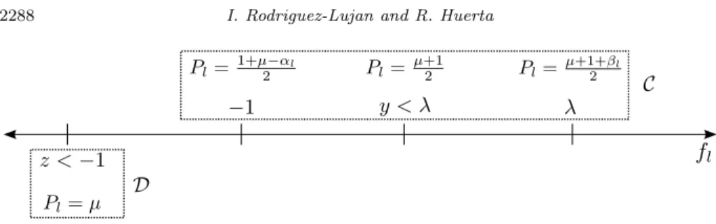
Proof. A detailed proof can be found in AppendixA. The sketch of the proof can be outlined as follows: forλ≤L−1, it is shown that the optimal decision functions are lower bounded by−1, while forλ > L−1 the decision functions are upper bounded byλ. Taking into account these bounds together with the sum-to-zero constraint, the minimization problem in Eq. (6) is formulated as an optimization problem with equality and inequality constraints. Then, the relationships between decision functions and class probabilities, which allow us to determine the classification calibration properties of our loss functions, are stated by the Karush—Kuhn—Tucker (KKT) conditions [5].
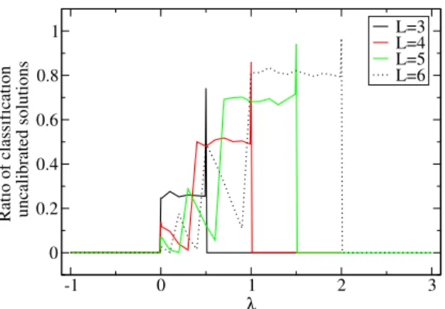
According to Theorem 2, we can define classification calibrated multiclass hinge loss functions for any multiclass classification problem by means of the scalar parameter λ. Certain values of λ enable not only to have classification calibrated loss functions, but also, unlike the other classification calibrated loss function [23], to take into account the margin of positive points. Figure2shows the ratio of classification uncalibrated solutions obtained by Monte Carlo sim-ulations for different values of the control parameter λ and the number of classes L. These results were obtained by counting the number of classifica-tion uncalibrated cases when minimizing the empirical Ψ-risk in Eq. (6) for 10,000 random probability simplex in RL. Monte Carlo simulations give ev-idence of the classification calibration domain presented in Theorem 2: λ ∈
Fig 2. Monte Carlo simulation results on the minimization of the empiricalΨ-risk associated
with our multiclass loss functions with variable marginλ. Figure shows the ratio of classifi-cation uncalibrated cases as a function of the control parameterλ and for different number of classesL. The number of simulations was set to 10,000.
5. Classification calibration for Support Vector Machines
Large-margin classifiers make tractable the minimization of the 0-1 loss by using convex surrogate loss functions. Examples of this approach are Support Vector Machines [8] and boosting [13]. The general formulation of a large-margin clas-sification algorithm with regularization is minf∈F (1/N)Ni=1Ψyi(f(xi)) + ρJ(f), where J(f) is a regularization term to penalize the model complexity, andρis the regularization parameter. Our proposed loss functions can be used in any standard regularized empirical risk minimizer. We used the Sequential Minimal Optimization (SMO) implementation of the Inhibitory Support Vector Machines (ISVMs) [19] since, as described further down in this section, they implicitly produce sum-to-zero decision functions for any example, while stan-dard SVMs do not. For example, Lee et al.’s implementation of SVMs needs to explicitly add a sum-to-zero constraint not necessary in the ISVM implementa-tion [23]. The best feature of the ISVM is the easiness of the implementaimplementa-tion that allows a quick adaptation to any variable margin framework.
ISVM is an extension of SVM to provide a simple algorithm for multiclass classification by directly integrating the concept of inhibition into the SVM formalism. The objective of the inhibition mechanism behind the ISVM algo-rithm is to find a hyperplane associated with each class, {wj}Lj=1, that exerts
downward pressure on the rest hyperplanes while trying to maximize its gener-alization capability. ISVM decision function for classjevaluated in a data point
xi has the form
fj(xi) = wj,Φ(xi) −μ
L k=1
where Φ is a mapping function from the original input space to a higher-dimensional spaceV (feature space) where the optimal hyperplane is calculated. The parameterμis a scalar number that regulates the inhibitory term, which is the key difference with respect to standard SVMs. The optimal decision vector
f is determined by following the standard SVMs’ framework. The ISVM primal problem is expressed as min w 1 2w 2+ C N L N i=1 L j=1 ηij (8) s.t. ηij≥0 (9) yijfj(xi)−1 +ηij ≥0, (10)
wherewis the concatenation of the hyperplanes of each class,w= [w1, . . . ,wL],
{ηij} are the slack variables that provide room to handle the noisy data, and
yij takes the value 1 if the patternxi belongs to class j (i.e., yi =j) and−1
otherwise. Note that now the trade-off between the regularization term and the loss function is controlled by the cost parameter C instead of the regulariza-tion parameter ρ. To simplify the notation, in what follows we assume that the cost parameter C is already normalized by the number of training points (N) and the number of classes (L). Inhibitory Support Vector Machines use an input space formed byL concatenations of the original input spaceX, and they use a feature space that is the product space VL. Then, an input vec-tor χi ∈ RM L is formed by L concatenations of the original training pattern xi∈RM. The corresponding nonlinear transformation Υ(χ)∈ VL is defined as Υ(χ) = (Φ(x),Φ(x), . . . ,Φ(x)) (Ltimes), and Υj(χ) is the composition of Υ(χ)
with the projection operator onto thej-th coordinate subspace corresponding to thej-th class; that is, Υj(χ) = (0,0, . . . ,Φ(x), . . . ,0) with all coordinates except
thej-th equal to zero. The transformations Υ and Υj inherit many properties
from the mapping function Φ(x). In particular,
Υj(χi),Υj(χi) = I[j=j]Φ(xi),Φ(xi), (11)
Υj(χi),Υ(χi) = Φ(xi),Φ(xi), (12)
Υ(χi),Υ(χi) = LΦ(xi),Φ(xi). (13) Huerta et al. show that the optimal value for μ is μ = 1/L, which can be obtained directly from the minimization of the Lagrangian of Problem (8)–(10) [19]. They also show that, in that limit, ISVMs become a tight bound to prob-abilistic exponential models. The inhibition term, therefore, is the average over the evaluation of the hyperplanes of each class. Interestingly,μis dependent on the number of classes of the problem, but independent of the training points themselves. This result is especially appealing when working with multiclass margin vectors since it yields sum-to-zero decision functions without imposing additional constraints in the optimization problem. ISVM automatically em-bodies all the zero-sum loss functions:
L j=1 fj(xi) = L j=1 wj,Φ(xi) − 1 L L k=1 wk,Φ(xi) = L j=1 wj,Φ(xi) −L 1 L L k=1 wk,Φ(xi)= 0.
The loss function in Eq. (10) corresponds toλ= 1. Therefore, it is straight-forward to integrate the family of loss functions presented in Eq. (4)–(5) into the ISVM’s framework. It can be formulated as follows
minw 1 2w 2+C N i=1 L j=1 ηij (14) s.t. ηij ≥0 (15) −1−(λ−1)yij+ 1 2 +fj(xi)yij+ηij≥0 forλ∈R. (16) To obtain the solution to Problem (14)–(16), we compute its Lagrangian as follows L(w,η, μ,ζ,α) = 1 2w 2+C N i=1 L j=1 ηij− N i=1 L j=1 ζijηij (17) − N i=1 L j=1 αij yij[w,Υj(χi) −μw,Υ(χi)] −1−(λ−1)yij+ 1 2 +ηij
where the Lagrange multipliers are αij ≥0 andζij ≥0. The decision function
associated with the j-th class for a training pointxi (Eq. 7) is now expressed as fj(xi) = w,Υj(χi) −μw,Υ(χi). We calculate the partial derivatives of
Lwith respect to the primal variablesw,η, andμto make them equal to zero. It leads to αij = C−ζij (18) w = N i=1 L j=1 αijyij[Υj(χi)−μΥ(χi)] (19) 0 = N i=1 L j=1 αijyijw,Υ(χi) (20)
Then, as in [19, Appendix B], replacing Eq. (19) in Eq. (20) yields the optimal
μasμ= 1/L. Since the partial derivatives of the Lagrangian w.r.t.μandwdo not depend on λ, this reasoning is valid for anyλ∈R, and, thus, sum-to-zero decision functions are guaranteed for all λ∈ R. This property makes ISVM’s framework advantageous for implementing multicategory margin vectors.
Now, we obtain the ISVM dual problem by applying Eq. (18)–(19) and Prop-erties (11)–(13) to the Lagrangian in Eq. (17) withμ= 1/L. It leads to the dual cost functionW that has to be maximized with respect to the Lagrange multi-pliers,αij, max α W = N i=1 L j=1 αijlij− 1 2 N i=1 L j=1 N i=1 L j=1 αijyijαijyijKii I[j=j]− 1 L , s.t. 0≤αij ≤C,
where lij = 1 + (λ−1)yij2+1 and Kii = K(xi,xi) = Φ(xi),Φ(xi). Now,
the decision function for thej-th class can be written in terms of the Lagrange multipliers and the kernel function as
fj(x) = N i=1 L j=1 αijyijK(xi,x)I[j=j]− 1 L N i=1 L j=1 αijyijK(xi,x).
We can simplify the evaluation by just computing
fj(x) = N i=1
αijyijK(xi,x) (21)
since the remaining terms simply add the same constant to all the classes. The class of the test sample xis defined as arg maxjfj(x). Following the notation
in [19], we change the double index notationαij for a new indexkrunning from
1 toN L. Assuming lexicographical order in theαijs, the dual cost functionW
can be written as max α W = N L k=1 αklk− 1 2 N L k=1 N L k=1 αkykαkykGkk (22) s.t. 0≤αk≤Cfor allk= 1, . . . , N L, (23)
whereGkk=K((k−1)/L)+1,((k−1)/L)+1I[(k modL)=(k modL)]−1/L. Then, it is easy to see that the KKT conditions for theλ-SVM training problem are
Vk≥0 forαk = 0,
Vk= 0 for 0< αk < C ,
Vk≤0 forαk =C ,
whereVk=yk(fk−lkyk) =ykfl−lk=ykfk−(1 + (λ−1)((yk+ 1)/2). Huerta
et al. provide a very easy and simple implementation of ISVM withλ= 1 based on Sequential Minimal Optimization (SMO) [30] that can be easily translated to the variable margin setting with minimal changes in the computer program. As originally proposed by Platt [30], the resolution of the proximity to the KKT condition in the optimization algorithm is controlled by a tolerance parameter
T > 0 and a numerical resolution, which depends on the machine precision. Then, the fulfillment of the KKT conditions is formulated as follows
Vk≥ −T forαk< , (24)
−T <|Vk|< T for < αk< C− , (25)
Vk< T forαk> C− . (26)
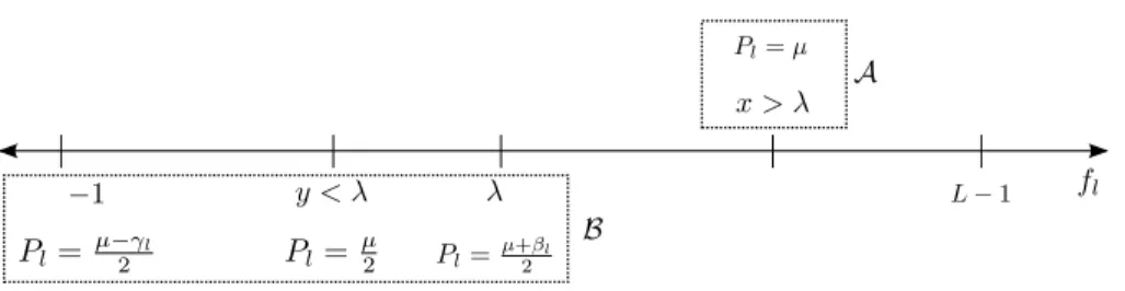
An interesting point of analysis is to determine the stability of the SMO optimization algorithm by taking into account the different regions of optimal decision functions defined by λand summarized in Figure3 (for more details, the reader is referred to Appendix A). Note that since SMO is used as opti-mization algorithm,λ-SVM optimal decision functions are defined as a function of the optimal Lagrange multipliers ˆαjs according to Eq. (21), which can be
easily obtained by means of the equality Vi = yi( ˆfi −liyi). To illustrate the
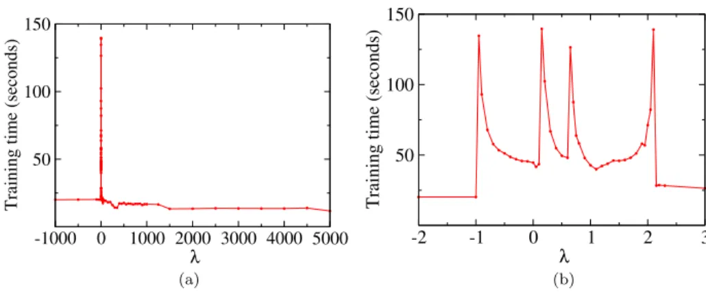
negative effect of having different KKT solutions in the proximity ofλin terms of computational cost, we measured the training times in the simplest case in which SMO is applied to single point. We set class probabilities toP1= 0.375,
P2 = 0.34, and P3 = 0.28, we created N = 264 training points, and we set
T = 10−3, = 10−6, and C = 106. The resulting training times for different λ-regions are shown in Figure3.
The different KKT conditions derived from Figure3together with the KKT numerical conditions in Eq. (24)–(26) allow us to formulate the following propo-sition.
Proposition 3. The optimal solution for the SVMs with variable margin has three possible KKT solutions in the domainλ∈(L−1−T, L−1 +T)for any resolution proximity T >0:
i) V1ˆ = 0 and 0 < α1ˆ < C ; V2ˆ ≤ 0 and α2ˆ = C; {Vˆj}Lj=3 = 0 and 0 < {αˆj}Lj=3< C.
ii) V1ˆ ≥0 andα1ˆ = 0;{Vˆj}jL=2= 0and0<{αˆj}Lj=2< C.
iii) V1ˆ = 0 and0<α1ˆ < C ;{Vˆj}Lj=2−1= 0and0<{αˆj}Lj=2−1< C ;VˆL≥0and
ˆ
αL = 0.
The resolution proximity T in the KKT conditions (Eq. (24)–(26)) implies to solve the dual problem for an effective marginλeff∈(λ−T, λ+T). That is why the SMO algorithm shows a slow convergence forλin the proximity of the boundary between different KKT solutions. It should also be noted that there may exist other points subject to KKT variations inside the same classification calibration region since the solutions forλ∈(−1,0) andλ∈((L−2)/2, L−1) depend on the class probability distribution, which in turn depends on λ. This is not the case for λ > (L−1) since the transition between the two possible solutions is only defined by the class probabilities; that is, the KKT conditions are constant given any λ >(L−1) and any point. It means that the margin
λ = (L−1) imposed by the reinforced multicategory hinge loss [28], though guaranteeing classification calibration, may slow down the convergence of the the SMO algorithm given that the optimizer is searching across different KKT
2270 I. R o driguez-Lujan and R .
Fig 3. Training times of the SMO algorithm trained with a single pointxas a function of the λ-regions defined by the classification calibration
Fig 4. Training times of SMO as a function of the margin of positive pointsλfor a single point
with class probabilitiesP1= 0.375,P2 = 0.34, andP3= 0.28. Figure4a shows the training
times forλ∈[−1000,5000]. Figure4b provides detailed training times forλ∈[−2,3].
regions. Proposition 3 and Figure 3 suggest that the margin of the positive points should be chosen somewhere in (−∞,−1)∪(L−1,+∞) with enough space with respect to the toleranceT to not incur in KKT instability problems. The caseλ∈(−∞,−1) corresponds to Lee et al.’s loss function [23]. However, values ofλ(L−1) provide the best training times as shown in Figure4. The advantage of strongly considering the margin of the positive points in terms of training times will be also confirmed in the following section.
6. Experimental evaluation
The aim of this section is to conduct an empirical evaluation in terms of classifi-cation accuracy and training times of theλ-SVM model introduced in Section5. We used four real-world datasets from the UCI data repository [24] described in Table 1. Some of these datasets involve real applications such as classification on gas sensor arrays [32]. Base error was obtained by predicting the majority class in each dataset. In Covtype dataset, a random selection of 50,000 points was performed. In the Abalone dataset, age bands were obtained dividing age by 5. These datasets were chosen because they have a large number of training points compared to the dimensionality. This favors large values of the cost pa-rameterC, which in turn can reveal differences between classification calibrated and uncalibrated loss functions since the regularization term almost vanishes. Otherwise, under appropriate regularization, all SVM models are classification calibrated [36].
We generated five different partitions of each experiment. The first 90% of samples was selected as the training set, and the remaining 10% of samples constituted the test set. The training samples were used to build the λ-SVM model. We used a function with compact support as a kernel. Kernels with non-zero tails such as the Gaussian kernel can be detrimental in scenarios with finite number of points and C very large since points that are significantly far from
Table 1
Datasets used to evaluateλ-SVMs
Dataset no. examples no. classes no. attributes Base error
Sensor 13,910 6 128 78.37%
Pendigit 10,992 10 16 89.59%
Covtype 50,000 7 54 51.24%
Abalone 4,177 6 8 51.59%
the point of interest can still have a notable contribution, especially when there are not enough points in the neighborhood of the point of interest. Specifically, we used the compactly supported kernel proposed and analyzed in [15,16,41]. The compactly supported kernel can be written as follows
KD,ν(x,x) = φD,ν(x,x)K(x,x), and, φD,ν(x,x) = 1−x−x D + ν ,
whereK(x,x) is the Gaussian kernel,D >0, and ν≥ M2+1 (M is the number of features). This kernel preserves positive definiteness as shown in [16]. The functionφD(·) induces sparsity since all entries satisfyingx−x ≥Dare set
to zero in the kernel matrix. Therefore, the constantDis called the thresholding or truncation parameter as it regulates the support size of the kernel KD,ν.
The parameterν controls the degree of smoothness or differentiability ofφD,ν.
Different choices of D and ν produce different compactly supported kernels. WhenD →0,KD,ν(x,x) evaluates as zero for every x=x, and it is equal
to 1, otherwise. WhenD→ ∞,KD,ν(x,x) recovers the Gaussian kernel. Since
the value ofν has no influence in the sparsity of the kernel, it is generally fixed at some value [41]. In this paper, we fixedν=M+1
2 in order to ensure positive
definiteness. We normalized the parameter γ, which determines the Gaussian kernel width, by the number of features:K(x,x) = exp
−γ
Mx−x
2
. We defined D as a function ofγ as followsD = (γ/M)−1 to reduce the number
of parameters to adjust by cross validation. The intuition behind the definition ofD is to maintain certain consistency between the Gaussian kernel width and the support size. The wider the Gaussian kernel, the larger support size.
The optimal cost parameterCand kernel widthγwere those with the lowest error when performing 10 cross–validation on the training set. The cost param-eter took values in the grid {10i | i= 0,1, . . . ,7}, and the kernel width γ was selected from the grid{10i|i=−3,−2, . . . ,3}. The test set was used to report a reliable estimation of the performance of the model. The algorithm used a tolerance level of T = 5·10−2 to exit. We imposed a training time limit of
2,500 seconds for the Sensor, Pendigit and Abalone datasets, and a time limit of 4,000 seconds for the Covtype dataset. We used our C++ implementation ofλ-SVMs, which is provided as Supplementary Material. The Matlab code for
Table 2
λ-SVMs classification error rates and training times.Ldenotes the number of classes in the dataset. Lee et al. [23], Huerta et al. [19] and Liu and Yuan [28]’s loss functions are indicated as Lee, ISVM, and RML (Reinforced Multicategory Loss), respectively. Loss function withλ= 0.1and ISVM loss function represent classification uncalibrated scenarios for these datasets. Classification errors and training times correspond to those values of the cost parameter (C opt.) and kernel width (γopt.) with the lowest cross-validation error. Training times marked with(∗)correspond to cases in which the cross validation runs did
not finish in the time limit for the largest values ofC λ -10,000 0.1 1 (L-1) 100 1,000 10,000 Lee ISVM RML Sensor Err.(%) 0.56 0.42 0.43 0.46 0.55 0.45 0.35 ±0.13 ±0.08 ±0.10 ±0.10 ±0.11 ±0.11 ±0.07 Time (s) 282 287 291 134 75 79 106 Copt. 3·106 1·106 3·106 3·106 8·106 2·106 1·105 γopt. 0.0600 0.0600 0.0700 0.0700 0.2700 0.9500 0.9500 Pendigit Err.(%) 0.36 0.44 0.36 0.35 0.27 0.76 0.82 ±0.10 ±0.09 ±0.06 ±0.09 ±0.07 ±0.15 ±0.13 Time (s) 1141(∗) 1180(∗) 1088(∗) 747 60 35 158 Copt. 1·107 1·107 8·106 8·106 1·107 1·107 3·105 γopt. 0.0260 0.0255 0.0260 0.0215 0.0450 0.4300 1.0000 Covtype Err.(%) 13.47 13.47 13.45 13.47 13.44 13.44 13.44 ±0.11 ±0.09 ±0.11 ±0.11 ±0.09 ±0.09 ±0.09 Time (s) 830(∗) 854(∗) 847(∗) 798 1230 1225 1227 Copt. 4·104 1·104 1·105 4·104 1·107 1·107 1·107 γopt. 2.5000 2.5000 2.5000 2.5000 2.5000 2.5000 2.5000 Abalone Err.(%) 29.43 31.15 30.43 29.23 29.86 29.81 31.24 ±1.05 ±0.76 ±1.17 ±1.01 ±1.10 ±1.03 ±0.92 Time (s) 247 350 359(∗) 221 164 30 6 Copt. 8·105 1·106 1·106 8·105 1·107 1·107 2·106 γopt. 0.0206 0.0026 0.0005 0.0023 0.0007 0.1000 2.2000
Table2shows the average classification errors and training times (in seconds) over the five test sets when different values ofλare considered in the loss func-tion. Results correspond to the optimal cost parameter C (C opt.) and kernel width γ (γ opt.) determined by cross–validation. The values of λ were chosen to have different classification calibration scenarios according to the analysis presented in Section4. Recall thatλ <−1 recovers the classification calibrated loss function originally proposed by Lee et al. [23], λ = 1 provides the ISVM loss function [19], andλ= (L−1) is equivalent to the reinforced multicategory hinge loss [28].
The minimum classification error is always achieved by a classification cal-ibrated loss function with λ ≥ (L −1). In general, classification errors for
λ ≥ (L−1) are either lower or similar to those corresponding to classifica-tion uncalibrated scenarios, while training times are usually lower. For example, given the optimal Candγ for each value ofλin the Pendigit dataset,λ-SVMs
Fig 5.λ-SVM results training times (in seconds) as a function of λfor different values of
the cost parameterC. Results for the mode of the kernel parameterγwith the lowest cross-validation error for eachλandCare shown. Lee et al. [23], Huerta et al. [19], and Liu and Yuan [28]’s loss functions are indicated as Lee, ISVM, and RML (Reinforced Multicategory Loss), respectively.
with large λ are at least 7 times faster than λ-SVMs with smaller values of
λ. Classification rates for the other classification calibrated loss corresponding to λ < −1 are competitive, but training is slower than for λ≥(L−1). This emphasizes the importance of counting the margin of positive points in the loss function in contrast to [28]. Moreover, the fact that training did not finish for the smallest values of λ in several datasets also corroborates the remarkable relevance of shifting overweight onto the margin of the positive points. It should be noted that in the Covtype dataset, the training times for λ(L−1) are the highest since the optimal cost parameter C is set to 107 in these cases; however, the lowest values ofλdid not explore the completeC grid given that they expired the training time limit. The following analysis of training times as a function ofλfor a givenγandCwill show the advantages of takingλ(L−1) in terms of computational cost.
Figure 5 shows the average training times for different values of the cost parameterCas a function ofλ. In order to have comparable training times, the mode of the optimal kernel parameterγ across all the cross validation runs is chosen for each dataset. Figure5shows that the training times forλ(L−1) are significantly lower than those corresponding to loss functions with negative
λorλin the interval ((L−2)/2,(L−1)). Differences are especially noticeable for the largest values of the cost parameterC. This result proves the advantage of strongly overweighting the margin of the positive points, and makes preferable the use of λ (L−1) instead of λ < −1 (Lee et al. loss function), λ = 1 (ISVM), or λ = (L−1) (reinforced multicategory). Finally, the long training times observed for λ in the interval ((L−2)/2,(L−1)) and in the proximity of λ= (L−1) are presumably due to the presence of different KKT regions as analyzed in Section 5. Thus, avoiding values for λin or close to the interval ((L−2)/2, L−1) is strongly recommended.
In short, our classification calibrated loss functions not only provide consis-tency guarantees that are directly reflected in the performance of the classifi-cation models, but they also provide excellent training times when the error of the positive points is significantly overweighted. A good value for λ should be large enough to strongly consider the margin of the positive points and safely keep away from the region where transitions between different families of solu-tions are possible. For example, settingλ= 100Lseems an appropriate choice in terms of classification calibration and training times according to our exper-imental results. Nevertheless, the best value forλshould ideally be determined empirically for each dataset by cross validation.
6.1. Comparison with other multiclass-SVM implementations
The aim of this section is to compare our multiclass loss function in terms of classification accuracy and computational times with other multiclass SVMs implementation and other loss functions different from those that can be treated as special cases ofλ-SVM. In this section, we compare the λ-SVM solver with the MSVMpack package [21], an open source software package that implements the generic multiclass SVM formulation proposed by Guermeur [17]. MSVMpack uses a Quadratic Programming solver based on the Frank-Wolfe method [12], and each step of the descent is obtained by solving a linear program (LP) by means of thelp solvesolver [29]. MSVMpack implements four multiclass loss functions: Weston and Watkins [39], Crammer and Singer [9], Lee et al. [23], and Guermeur and Monfrini [18]. For more details about the MSVMpack package, the reader is referred to [21].
We followed the same experimental setup described in Section6. We included the kernel with compact support in the MSVMpack implementation thanks to the flexibility of this software package to customize kernel functions. The Covtype dataset is not included in the comparison given its high computational cost. Both implementations, MSVMpack andλ-SVMs were configured to run in one single processor in order to better control the computational times. Please, note that our goal is not to compete with the excellent implementation provided by MSVMpack, but to provide insight into SVMs’ multiclass loss functions in terms of classification calibration properties and computational cost. The results for MSVMpack for the Sensors, Pendigit, and Abalone datasets and the four loss functions (Weston and Watkins, Crammer and Singer, Lee et al., and Guermeur and Monfrini) are shown in Table3.
Table 3
MSVMpack classification error rates and training times. Weston and Watkins [39], Crammer and Singer [9], Lee et al. [23], and Guermeur and Monfrini [18]’s loss functions are indicated as WW, CS, Lee, and MSVM2, respectively. Classification errors and training
times correspond to those values of the cost parameter (Copt.) and kernel width (γopt.) with the lowest cross-validation error
Loss function WW CS Lee MSVM2 Sensor Err.(%) 0.53±0.07 0.65±0.11 0.61±0.05 0.46±0.03 Time (s) 612±13 249±15 804±9 1225±16 Copt. 5·105 1·105 105 1·106 γopt. 0.0004 0.0035 0.0009 0.0001 Pendigit Err.(%) 0.27±0.08 0.36±0.09 0.31±0.07 0.29±0.08 Time (s) 2500±0 113±3 760±13 1246±5 Copt. 2·106 1·105 1·105 8·105 γopt. 0.0340 0.0170 0.0600 0.0500 Abalone Err.(%) 30.74±1.10 30.27±0.86 30.74±1.28 30.12±1.00 Time (s) 32±4 24±4 112±2 91±4 Copt. 8·103 6·104 3·105 5·104 γopt. 0.6200 0.0226 0.0040 0.0015
MSVMpack classification rates are similar to those obtained byλ-SVM. When the optimal λ is chosen in Table 2, λ-SVMs classification rates are equal or higher than those obtained by any of the loss functions implemented by MSVM-pack. This means that using our loss function only can improve the classifica-tion accuracy. Regarding the training times, in general, λ-SVMs are faster for large values of λwhile maintaining competitive classification accuracies. Since MSVMpack andλ-SVMs implement Lee et al.’s loss function, both implementa-tions can be compared. For Lee et al.’s loss function, experimental results show that (i) MSVMpack andλ-SVM provide similar results; and (ii) training times are dataset-dependent: MSVMpack implementation is faster that λ-SVM im-plementation in the Pendigit and Abalone datasets, whileλ-SVM is faster than MSVMpack in the Sensors dataset. Overall, these experimental results show the efficiency of MSVMpack implementation, but they also reveal that there is still room for improvement in the loss function itself.
7. Conclusions
In this paper, we have proposed a family of multiclass hinge loss functions regulated by a control parameter λ that controls the margin of the positive points of a given class. These surrogate loss functions, Ψy, exhibit different
classification calibration properties as a function ofλ. We have determined the values ofλfor which the proposed loss functions are classification calibrated, and we have shown that our family of loss functions allows us to define a classification calibrated hinge loss function for every multiclass classification problem. Unlike other classification calibrated hinge loss functions, we can give arbitrarily high
weight to the margin of the positive points, which is empirically shown to be positive for learning. Our family of loss functions is general enough to recover Lee et al. [23] and Liu and Yuan [28]’s classification calibrated loss functions by settingλ≤ −1 andλ= (L−1), respectively, withLthe number of classes. However, we show that other values of λallow overcoming some limitations of previous approaches while maintaining classification calibration properties.
We have embedded our family loss functions in the Support Vector Ma-chine’s formalism (λ-SVM) and implemented a Sequential Minimum Optimiza-tion (SMO) algorithm. We have shown that the optimizaOptimiza-tion algorithm has different convergence rates that can be explained in terms of the classification calibration domain and the different families of SVMs’ solutions and KKT con-ditions defined by λ. In particular, values of λ (L−1) provide the fastest convergence while guaranteeing classification calibration.
We have compared the performance of λ-SVMs in four real-world datasets to conclude that classification calibrated loss functions considering the margin of positive points only can improve classification uncalibrated loss functions in terms of classification accuracy. Additionally, λ-SVMs with large values for λ
exhibit the lowest training times, which matches with our theoretical analysis of SMO’s solutions. These results reveal the importance of strongly overweighting the positive samples in the learning process.
In conclusion, a value of λ large enough would guarantee classification cal-ibration while taking the maximum advantage of the positive examples and providing good convergence rates. Though the optimal value for λ should be determined in a validation phase, our theoretical and empirical results indicate that λ= 100L is a good choice. It not only ensures classification calibration, but it also provides good classification performance and training times. Appendix A: Detailed proof of Theorem 2
This Appendix provides a detailed proof of Theorem 2. In what follows, we assume that class probabilities {P1, P2, . . . , PL} for a point x are all different
and ordered as P1 > P2 > . . . > PL, and let f1, f2, . . . , fL be the decision
functions associated with these class probabilities. Before addressing the proof, let us formulate two properties of our loss function that make the classification calibration analysis more tractable.
Property 4. Ψy(f(·)) satisfies arg minj{Ψj(f(xi))} = arg maxj{fj(xi)} =
pred(xi).
Property 5. Given the ordered class probabilities P1 > P2 > . . . > PL, the
minimizer fˆof Eq. (6) must verify: fˆ1≥fˆ2≥. . .≥fˆL.
The proof of Theorem2 is the result of the combination of Lemmas6–8. Lemma 6. Given a multiclass classification problem with L classes, the λ -parametrized family of loss functions defined in Eq. (4)–(5) is classification cal-ibrated for λ <−1.
Proof. Firstly, we show that the minimizerfˆof Eq. (6) is lower bounded by−1 forλ <−1. The solutionf1=L−1 andf2=f3=. . .=fL=−1 is a feasible
solution lower bounded by−1, and it evaluates as (1−P1)Lin Eq. (6). Letf1
be another solution withf1
j <−1. We obtain the following chain of inequalities
for the objective function in Eq. (6)
L l=1 Pl[λ−fl1]++ (1−Pl)[1 +fl1]+ = L l=1 Pl[λ−fl1]++ l=j (1−Pl)[1 +fl1]+ ≥ l=j (1−Pl)[1 +fl1]+≥ l=j (1−P1)(1 +fl1) = (1−P1)(L−1−fj1)≥(1−P1)L .
Then, any solution withfj <−1 produces a larger value in the Ψ-risk than
the solution f1 = L−1;f2 = f3 = . . . = fL = −1, and, thus, it cannot be
minimizer. Therefore, in what follows, we only need to considerf withfj ≥ −1
for allj= 1, . . . , L. Imposing the sum-to-zero constraint,Ll=1fl= 0, we obtain
the following inequalities for allfj
−1≤fj≤L−1, (27)
and, thus, all the terms [λ−fl]+in Eq. (6) vanish, and the problem is equivalent
to that proposed by Lee et al. in which the positive examples of a class do not take part in the loss function [23]. This case has already been shown to be classification calibrated [23, 26]. We include the proof for completeness’ sake. Forλ <−1, the following equality holds
min f L l=1 Pl[λ−fl]++ (1−Pl)[1 +fl]+ = min f L l=1 (1−Pl)(1 +fl) = (L−1)−min f L l=1 Plfl.
Consequently, minimizing Eq. (6) is equivalent to maximizing Ll=1Plfl.
Then, the problem reduces to max f L l=1 Plfl, s.t. L l=1 fl= 0, fl≥ −1 for l= 1,2, . . . , L . (28)