Study on proximal support vector machine as a classifier

(1)

STUDY ON PROXIMAL

SUPPORT VECTOR MACHINE

AS A CLASSIFIER

A THESIS SUBMITTED IN PARTIAL FULFILLMENT

OF THE REQUIREMENT FOR THE DEGREE OF

Master of Technology

In

Electronics and Instrumentation

By

DEEPIKA ORAON 210EC3326

Department of Electronics and Communication Engineering National Institute Of Technology, Rourkela

Orissa 769008, India 2012

(2)

STUDY ON PROXIMAL

SUPPORT VECTOR MACHINE

AS A CLASSIFIER

A THESIS SUBMITTED IN PARTIAL FULFILLMENT

OF THE REQUIREMENT FOR THE DEGREE OF

Master of Technology

In

Electronics and Instrumentation

By

DEEPIKA ORAON 210EC3326

Under the Guidance of

Dr. Samit Ari Assistant Professor

Department of Electronics and Communication Engineering National Institute Of Technology, Rourkela

Orissa 769008, India 2012

(3)

Dedicated to

(4)

Department of Electronics and Communication Engg

National Institute of Technology Rourkela

Rourkela-769008, Orissa, India.

June 4, 2012

Certificate

This is to certify that the work in the thesis entitledStudy On Proximal Support Vector Machine As A Classifier by Deepika Oraon is a record of an original research work carried out under my supervision and guidance in partial fulfillment of the requirements for the award of the degree of Master of Technology in Electronics and Communication Engineering. Neither this thesis nor any part of it has been submitted for any degree or academic award elsewhere.

Place: NIT Rourkela Dr. Samit Ari

Date: June 4, 2012 Assistant Professor

Department of EC NIT Rourkela

(5)

Acknowledgment

With the making of this thesis, I first express my sincere gratitude to my project guide Dr. Samit Ari, Assistant Professor, Department of Electronics & Communication, NIT, Rourkela for his persistent pioneer at every single step conducing to the successful completion of the thesis. At every stage, I encountered doubts and problems; he dispelled them away with his consistent guidance and ad-vises. He was a real source of inspiration for me throughout the making of the project.

I express my obligation to Dr. Sukadev Meher, Head of Department, Elec-tronics & Communication, NIT, Rourkela for availing me all the facilities to accomplish the project in the department itself.

I am grateful to all faculty members and the supporting staff members of the de-partment of Electronics & Communication for their constant support and motivation in the making of the thesis.

I thank my parents, husband & friends for being the eternal source of moral sup-port & motivation and to almighty God for blessing me with the zeal and endeavor to work towards my goal.

(6)

Abstract

Proximal Support Vector machine based on Least Mean Square Algorithm classi-fiers (LMS-SVM) are tools for classification of binary data. Proximal Support Vector based on Least Mean Square Algorithm classifiers is completely based on the theory of Proximal Support Vector Machine classifiers (PSVM). PSVM classifies binary pat-terns by assigning them to the closest of two parallel planes that are pushed apart as far as possible. The training time for the classifier is found to be faster compared to their previous versions of Support Vector Machines. But due to the presence of slack variable or error vector the classification accuracy of the Proximal Support Vector Machine is less.

So we have come with an idea to update the adjustable weight vectors at the train-ing phase such that all the data points fall out-side the region of separation and falls on the correct side of the hyperplane and to enlarge the width of the separable region. To implement this idea, Least Mean Square (LMS) algorithm is used to modify the adjustable weight vectors. Here, the error is represented by the minimum distance of data points from the margin of the region of separation of the data points that falls inside the region of separation or makes a misclassification and distance of data points from the separating hyperplane for the data points that falls on the wrong side of the hyperplane. This error is minimized using a modification of adjustable weight vectors. Therefore, as the number of iterations of the LMS algorithm increases, weight vector performs a random walk (Brownian motion) about the solution of optimal hy-perplane having a maximal margin that minimizes the error. Experimental results show that the proposed method classifies the binary pattern more accurately than classical Proximal Support Vector Machine classifiers.

Keywords: Data classification, least mean square (LMS), least square support vec-tor machine (LS-SVM), proximal support vecvec-tor machine (PSVM), support vecvec-tor machine (SVM).

(7)

Notations and terms

Some words about notations which are used in our work. All vectors are treated as

column vectors unless transposed to a row vector by a prime superscriptT. The inner

(scalar) product of two column vectors xand y in the real n-dimensional spaceRn _is

denoted by xT_y_{, and} _||_x_|| _{represents the 2-norm of} _x_{. For the matrix} _A _∈_Rm×n_, _A i

is the ith row of A which is a row vector in Rn. A column vector of ones of arbitrary

suitable dimension is denoted by column matrixeand the identity matrix of arbitrary

suitable order is denoted byI. The kernel function is denoted byφ(x). The Gaussian

kernel function is denoted by K(x, C) where C is the set of centers. exp is the base

(8)

List of Figures

2.1 Optimal separating hyperplane . . . 6

2.2 Maximum margin hyperplane . . . 7

2.3 Architecture of SVM . . . 8

2.4 Support vector machine (SVM) . . . 9

2.5 SVM with slack variable or error vector . . . 10

2.6 The Proximal Support Vector Machine Classifier . . . 14

4.1 The ideal Proximal Support Vector Machine Classifier in the (ω, b )-space of Rn+1. The planes ωTx−b =±1 around which points of the sets +1 and -1 cluster and which are pushed apart by the optimization problem (4.2). . . 31

4.2 The Proximal Support Vector Machine Classifier in the (ω, b)-space of Rn+1_{. The planes} _ωT_x₋_b ₌ _±_{1 around which points of the sets +1} and -1 cluster and which are pushed apart by the optimization problem (4.2). . . 31

(9)

4.3 The proposed lms based proximal support vector machine classifier,

after training the datasets lie outside the margin and on the correct

(10)

List of Tables

2.1 Results of SVM as linear classifier for average 10-fold accuracy test

with and without shuffling . . . 15

2.2 Results of LS-SVM as linear classifier for average 10-fold accuracy test

2.3 Results of SVM as a linear classifier for average 10-fold accuracy test

with shuffling . . . 16

2.4 Results of SVM as a linear classifier for average 10-fold accuracy

with-out shuffling . . . 16

2.5 Results of PSVM as a linear classifier for average 10-fold accuracy test

with shuffling . . . 17

without shuffling . . . 17

2.8 Results of average 10-fold accuracy test using nonlinear kernel without

(11)

2.9 Results of PSVM for average 10-fold accuracy test using nonlinear

ker-nel with shuffling . . . 18

3.1 Cancer datasets used for results and comparison in our experiment. . 23

3.2 Details about other datasets used for results and comparison in our

experiment. . . 24

4.1 Results of average 10-fold accuracy test using linear kernel without

shuffling . . . 34

4.2 Results of average 10-fold accuracy test using linear kernel with

shuf-fling . . . 34

4.3 Results of average 10-fold accuracy test using linear kernel with

shuf-fling . . . 35

4.4 Results of average 10-fold accuracy test using linear kernel without

shuffling . . . 35

5.1 Results of cancer datasets for average 10-fold accuracy test using

non-linear kernel without shuffling . . . 43

5.2 Results of cancer datasets for average 10-fold accuracy test using

non-linear kernel with shuffling . . . 43

5.3 Results of UCI repository datasets for average 10-fold accuracy test

using nonlinear kernel without shuffling . . . 44

5.4 Results of UCI repository datasets for average 10-fold accuracy test

(12)

5.5 Time taken by the classifiers to train cancer datasets with reduced

kernel matrix size . . . 45

5.6 Time taken by the classifiers to train UCI repository datasets with

(13)

Chapter 1 Introduction

Motivation

Contribution

(16)

1.1 Motivation Introduction

1.1 Motivation

Support vector machines (SVMs) are example of machine learning. Machine learning is defined as the ability of a system to learn from its experience, i.e. to modify or update its processing based on the basis of newly acquired informations. In this thesis support vector machine is used as a classifier. The pattern used for classification have two classes. The main objective of the SVM is to design a hyperplane and separate the margin between the different classes. The SVM divides the space into two half spaces such that datapoints of different classes are separated. As the size of the patterns increases, the training time increases and also the computational complexity increases in case for SVM. In order to overcome the drawbacks of SVM, proximal support vector machine (PSVM) was developed. The classification accuracy of the PSVM is comparable to standard SVM but the computational complexity of PSVM is less than SVM. The training time required by PSVM is less as compared to large training time in case of standard SVM. PSVM assigns the classes to the datapoints by measuring its proximity from the two parallel hyperplanes. The datapoints are clustered around the two parallel hyperplanes. The hyperplanes should be designed such that the margin of separation between the two classes should be maximized. The tuning parameter of the optimal hyperplanes are obtained by optimization of the quadratic function. In PSVM equality constraint is used in place of the inequality constraint, which makes the computation cheaper. In order to remove the human effort automatic classification technique can be used.

The classification technique involved for approval of credit cards, detection of good or bad RADAR signal and other diseases can be done using an automatic classi-fier. This thesis considers the advance classification scheme to automatically classify datasets into two classes.

1.2 Contribution

This thesis aims to introduce an improved version of proximal support vector machine (PSVM). It can be used in fields like image based gender identification, handwritten

(17)

1.3 Organization of the thesis Introduction

digit recognition, bioinformatics, text categorization etc. This improved version of proximal support vector machine (PSVM) focuses on the pattern classification of binary datasets. It allows assessments of datasets and classifies the abnormal dataset from normal dataset, for example in case of Bupa liver datasets, it picks out the patients having a liver disorder from normal patients. The idea behind proposed work is to maximize the margin between the hyperplanes or the decision surface such that datapoints lie on the correct side of the hyperplanes in order to increase the generalization ability of the classifier or to minimize the generalization error. The minimum generalization error is described as when a new set of datapoints with unknown class labels arrive for the classification, the chances of occurring an error while predicting the class of datapoints based on the learning or hyperplane classifier should be minimum. The proposed work makes use of least mean square (LMS) algorithm, which modifies the weight vector during training time to reduce the training classification error. These modified weight vector is used after training for testing purpose. As compared to standard SVM and PSVM, the classification efficiency of proposed work is more. The effectiveness of the proposed work is verified by tests on several benchmark datasets for both linear and nonlinear classifiers.

1.3 Organization of the thesis

The thesis is organized as follows. Chapter 2 describes the experimental setup and datasets used in the proposed work. Chapter 3 provides details about the standard support vector machine (SVM) classifier, least square support vector machine (LS-SVM)and proximal support vector machine (PSVM)for linear and nonlinear classifier. Chapter 4 contains the proposed technique for linear classifier and the result of ex-periments performed on different datasets to check its efficiency. Chapter 5 extends the formulation of proposed method for nonlinear classifier. Chapter 6 presents the testing and comparison, conclusion and discusses points for further research.

(18)

Chapter 2 Introduction to SVM

Theoretical Background

Support Vector Machine

Least Square Support Vector Machine

Proximal Support Vector Machine

Experimental Results

(19)

2.1 Theoretical Background Introduction to SVM

2.1 Theoretical Background

Support vector machines (SVM) [1-4] are based on statistical learning theory [5]. They are supervised learning systems. SVM [1-4] proves to be an excellent statistical tool for classification as well as regression analysis as it can analyze and recognize the data very well. Due to its efficient implementations, SVM extends to many fields like handwritten digit recognition [6], text categorization [7], Bioinformatics [8] and image based gender identification [9]. The SVM was developed by Vapnik [5] to approximately reduce the error on the training data. As SVM was developed to implement SRM [10], which minimizes the upper bound on the expected risk that reduces the misclassification error and is able to generalize well. The idea of a support vector machine is to construct a decision surface in the form of a hyperplane that separates or set apart the datasets of two classes in such a way that the margin of separation [11] between the two classes is maximized. In case of the nonlinearly separable dataset, input data are projected into another high dimensional feature space [11], [12] with the help of kernel function which made the data separable in that space. After that SVM [1-4] finds a linear separating hyperplane in this higher dimensional space having the maximal margin. The decision surface is linear in the high dimensional feature space but it is nonlinear in input space. The parameters of the solution or optimal hyperplane are derived from the optimization of the cost function subjected to inequality constraints.

The performance and accuracy of the SVM classifier depend upon some tuning parameters [1], [2] which are selected during training time. SVM takes large training time in order to obtain the best tuning parameters for the optimal classifier, which reduces the performance and efficiency. In order to overcome this drawback many versions of SVM have been developed with comparable classification quality. Suykens et al. [13], [14] developed least square support vector machine classifier (LS-SVM), which considers equality constraints for the classification problem instead of inequality constraints as in case of classical SVM. As a result, the optimal hyperplane is obtained by solving a set of linear equations [13], [14] instead of a quadratic function as in the case of standard SVM. G. Fung and O. L. Mangasarian [15] proposed proximal

(20)

2.2 Support Vector Machine (SVM) Introduction to SVM

Figure 2.1: Optimal separating hyperplane

support vector machine (PSVM) based on assigning the dataset by measuring the distance of it from the two parallel hyperplane. Datasets closest to one of the two parallel hyperplane are assigned to the corresponding class of that hyperplane. PSVM formulation uses strong convex objective functions which are not found in the case of SVM [10], [16] and LS-SVM [13], [14]. Strong convexity [15] plays a key role for PSVM in the reduction of complex code to simple code and also very fast computational time is obtained due to its strong convexity during training.

In this chapter classifier such as SVM, LS-SVM and PSVM is discussed. This chapter also extended to nonlinear classifiers and the merits and demerits of classifiers over each other

2.2 Support Vector Machine (SVM)

Support vector machines (SVM) [1-4] are a powerful algorithmic approach to the prob-lem of classification and regression. A classification task mainly involves separating the datasets into training and testing sets. Each sample in the training set contains one “target value” (i.e. the class tag) and several “attributes” (i.e. the observed variables or features). The goal of SVM classifiers is to produce a model or a decision surface based on the training data, which recognizes the target value of the testing dataset.

(21)

Figure 2.2: Maximum margin hyperplane

2.2.1 Optimal Separating hyperplane

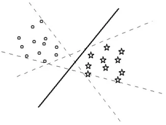
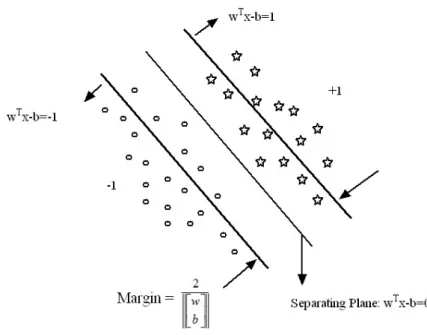
SVM firstly deal with the question of optimal hyperplane. In Fig. 2.1, the circle points and star points respectively represent class +1 and class -1. In Fig. 2.1 there are many possible hyperplane or classifier which can separate the datasets of class +1 and -1, but only one can maximizes the margin. Here margin is defined as the distance between the classifier and the nearest datapoint of each class. The bold line is an optimal hyperplane, which maximizes the margin as well as separate the datapoints successfully.

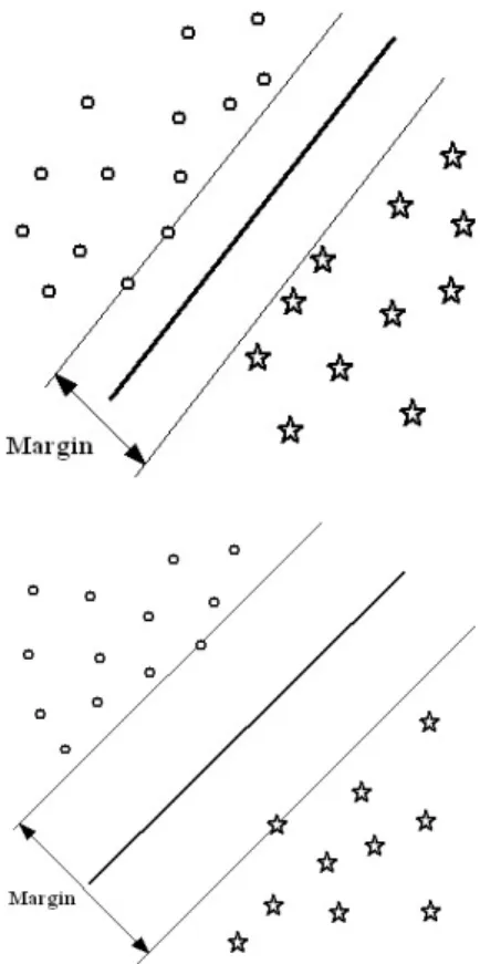
Fig. 2.2 represents the maximum margin hyperplane. The maximum margin hy-perplane increases the generalization ability. If the set of hyhy-perplane is able to separate the two classes without any errors then the experimental risk is small. Therefore, op-timal hyperplane means that a hyperplane which separate the two class clearly with maximum margin.

(22)

Figure 2.3: Architecture of SVM

2.2.2 Architecture of SVM

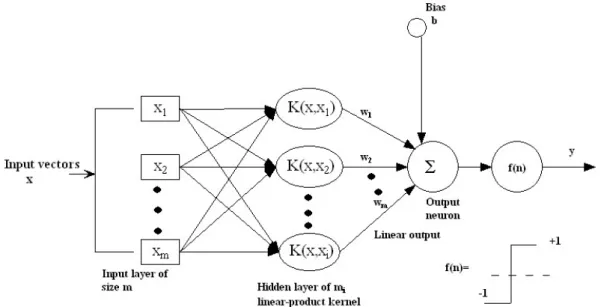
The architecture of SVM is shown in Fig. 2.3. As compared to neural network, support vector machine may be described as a feed-forward neural network having one hidden layer. Here, x1, x2, ..., xm are an input layer of size m. x is an input vector defined in n-real dimensional spaceRn, it contains elements likex1, x2, ..., xm. K(x, x1), K(x, x2), ..., K(x, xi) are hidden layer ofmi linear-product kernel. w is the weight vector having elements w1, w2, ..., wm. Output neuron is the output layer of the feed-forward neural network. b is bias defined in real dimensional space R. f(n) is decision function, which makes the final classification.

2.2.3 Formulation of SVM

Let the patterns to be classified denoted byx matrix inm×n real dimensional space and (x1, y1),(x2, y2), ....,(xm, ym) are the m training patterns, where xi denotes the attributes of the data whereasyidenotes the output or target value for the correspond-ing data. The decision boundary or the hyperplane for the classification purpose is defined as

ωTφ(x) +b = 0, (2.1)

(23)

Figure 2.4: Support vector machine (SVM)

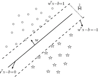
the bias term of the hyperplane. The hyperplane is constructed such that it satisfies the following inequality functions for both the classes. Fig. 2.4 shows the support vector machine.

ωTφ(xi) +b≥+1, if yi = +1, (2.2)

ωTφ(xi) +b ≤ −1, if yi =−1. (2.3)

which is equivalent to

yi[ωTφ(xi) +b]≥1, i= 1, ..., m. (2.4)

If the datapoints violate Eq. (2.4), in case a separating hyperplane in this higher dimensional space does not exist then a new set of non-negative slack variable (scalar variable) ξi is introduced such that

yi[ωTφ(xi) +b]≥1−ξi (2.5)

and ξi ≥0 (2.6)

The SVM with slack variable or error vector is shown in Fig. 2.5. The optimal hyperplane is obtained by minimizing the risk bound according to the structural risk minimization principle and this is done by formulating the optimization problem in Eq. (2.7). min ω,ξ J(ω, b, ξ) = 1 2||ω|| 2₊_c m X i=1 ξi (2.7)

(24)

Figure 2.5: SVM with slack variable or error vector

where c >0

where c is the regularization parameter that is used for balancing the importance of maximizing the margin and reducing the training error. The parameter c is deter-mined experimentally with the help of the standard use of a training or (validation) test set, which is a crude form of resampling. The above Eq. (2.5) and (2.7) can be written in the Lagrangian function as:

L(ω, b, ξi;αi, βi) = J(ω, b, ξi)−c m X i=1 αi[yi(ωTφ(xi) +b)−1 +ξi]− m X i=1 βiξi (2.8)

αi and βi are the Lagrange multipliers such that αi ≥0, βi ≥0 where i= 1,2, ...., m. The solution to the quadratic problem is obtained by solving saddled Lagrange func-tion. As a result one obtains the following conditions.

∂L ∂ω = 0 →ω= m X i=1 αiyiφ(xi), ∂L ∂b = 0 → m X i=1 αiyi = 0, ∂L ∂ξi = 0 →0≤αi ≤c, where i= 1,2, ..., m.                            (2.9)

(25)

2.2 Support Vector Machine (SVM) Introduction to SVM problem: max αi Q(αi;φ(xi)) = m X i=1 αi− 1 2 m X i,j=1 yiyjφ(xi)Tφ(xj)αiαj (2.10) such that m X i=1 αiyi = 0, 0≤αi ≤c, i= 1,2, ...., m. (2.11)

The function φ(xi) in Eq. (2.10) is related to K(x, xi) by imposing φ(x)Tφ(xi) = K(x, xi), which is motivated by Mercer’s theorem [13]. The classifier is designed by solving Eq. (2.12) max αi Q(αi;φ(xi)) = m X i=1 αi− 1 2 m X i,j=1 yiyjK(x, xi)αiαi (2.12) subject to m X i=1 αiyi = 0, 0≤αi ≤c, i= 1,2, ...., m. (2.13)

HereK(., .) represents the kernel function of x.

2.2.4 Kernel methods

Kernel methods algorithm is used for pattern analysis. The main characteristic of kernel is its distinct action to the problem of pattern classification of different types of data. Kernel methods represent the patterns in high dimensional feature space such that the patterns can be made more easily separated. The mapping is not subjected to any constraints, so kernel method can conduct to infinite-dimensional space for the purpose of classification. A tool called kernel trick is used in order to map the patterns in the higher dimensional space.

The kernel trick can be implemented to algorithms which depends upon dot prod-uct between two vectors. So, a dot prodprod-uct is replaced by a kernel function for map-ping of patterns. Replacing the linear algorithm by nonlinear algorithm is not altering their original working in feature spaceφ. The selection of correct kernel depends upon type of patterns available. There are following choices for kernel function:

(26)

2.3 LS-SVM Introduction to SVM

It is the most simple and easy to use kernel function. Linear kernel is represented as summation of inner product {x, xi} and an optional constant d.

K(x,xi) = xTxi+d

(ii) Polynomial kernel

Polynomial kernel is suitable for normalized datasets as it is a nonstationary kernel.

K(x,xi) = (βxTxi+d)p

pis polynomial degree,dis constant andβis slope. Polynomial degree, constant and slope can be adjusted according to the requirement.

(iii) Radial basis function

In this thesis Gaussian kernel is used, which is an example of radial basis func-tion. Gaussian kernel can be represented as

K(x,xi) = exp(

−||x−xi||2

2σ2 )

The adjustable parameter is sigma, it plays an important role in the performance of kernel function and should be selected carefully for the patterns available.

(iv) Hyperbolic tangent kernel

It is also known as the multilayer perceptron and as the sigmoid kernel. SVM model using sigmoid kernel function is equivalent to the two layer perceptron neural network.

K(x,xi) =tanh(βxTxi+d) (2.14)

The adjustable parameter are slope β and the constant d.

2.3 LS-SVM

The major drawback of the standard SVM [1-4] is that it takes large amount of training time. Suykenset al. resolved this problem by introducing least square support vector

(27)

2.4 PSVM Introduction to SVM

machine (LS-SVM) [13], [14]. LS-SVM is reformulation of standard SVM that leads to solving linear Karush-Kuhn-Tucker (KKT) [17] system. LS-SVM minimizes the least square error [13], [14] on the training patterns while simultaneously maximizing the margin between the two classes. The cost function of LS-SVM is as follow:

minω,ξJ(ω, b, ξ) = 1₂||ω||2+c m P i=1 ξ_i2 s.t yi(ωTφ(xi) +b) = 1−ξi (2.15)

In this case, the inequality constraint condition used for standard SVM is replaced by the equality constraints. The computational complexity reduces drastically as well as gives approximately the same accuracy. The lagrangian of the cost function can be defined as: L(ω, b, ξ :α) = J(ω, b, ξ)− m X i=1 αi[yi(ωTφ(xi) +b)−1 +ξi] (2.16)

αi is the lagrangian multiplier due to equality constraint. The conditions of opti-mality are obtained by differentiating the lagrangian function with respect to ω, b, ξ and α and equating it to zero is given as:

∂L ∂ω = 0 →ω = m X i=1 αiyiφ(xi), ∂L ∂b = 0 → m X i=1 αiyi = 0, ∂L ∂ξi = 0 →ξi =γyi, ∂L ∂αi = 0 →[yi(ωTφ(xi) +b)−1 +ξi] = 0, where i= 1,2, ...., m.                                      (2.17)

Therefore, the final solution for making decision is of the form:

f(x) = sign[ m X i=1 αiyiK(x, xi) +b] (2.18)

2.4 PSVM

In proximal support vector machine (PSVM) [15] instead of dividing the space into disjoint regions for each class, the data points are assigned according to the proximity

(28)

2.4 PSVM Introduction to SVM

Figure 2.6: The Proximal Support Vector Machine Classifier

to the hyperplanes that are separated as far as possible [15]. This leads to a very fast and simple algorithm [15]. The cost function is given as follows:

minω,b,ξJ(ω, b, ξ) = 1₂||[ω, b]T||2+₂c m P i=1 ||ξi||2 s.t. yi(ωTφ(xi) +b) = 1−ξi (2.19)

The minimization of cost function leads to maximization of margin in (ω, b) space. It also uses the equality constraint and minimizes the squared error like LS-SVM [13], [14]. The PSVM [15] works much faster than SVM [1-4] as well as give performance similar to SVM. The lagrangian of the cost function is given as:

L(ω, b, ξ :α) = J(ω, b, ξ)−

m

X

i=1

αi[yi(ωTφ(xi) +b)−1 +ξi] (2.20)

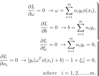
αi is the lagrangian multiplier due to equality constraint. The cost function is differ-entiated with respect to ω, b, ξ and α which gives:

(29)

2.5 Experimental Results Introduction to SVM ∂L ∂ω = 0 →ω = m X i=1 αiyiφ(xi), ∂L ∂b = 0 →b = m X i=1 αiyi, ∂L ∂ξi = 0 → m X i=1 αiyi = 0, ∂L ∂αi = 0 →[yi(ωTφ(xi) +b)−1 +ξi] = 0, where i= 1,2, ..., m.                                        (2.21)

The linear classifier to the linear separating surface is as follows:

ωTx−b          >0, then x∈+1, <0, then x∈ −1, = 0, then x∈+1 or x∈ −1. (2.22)

2.5 Experimental Results

Table 2.1: Results of SVM as linear classifier for average 10-fold accuracy test with and without shuffling

.

S.NO DATASET SVM (not shuffled) SVM (shuffled)

1. Colon (62x2000) 36.19±22.22 35.23±19.71 2. Lung (22x56) 43.33±47.25 40.00±30.91 3. ALL-AML (100x500) 72.50±42.50 71.66±13.54 4. Prostate (38x1000) 44.00±9.16 44.00±11.13

(30)

2.5 Experimental Results Introduction to SVM

Table 2.2: Results of LS-SVM as linear classifier for average 10-fold accuracy test with and without shuffling

.

S.NO DATASET LS-SVM (not shuffled) LS-SVM (shuffled)

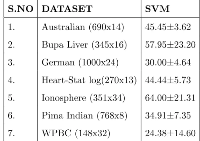
Table 2.3: Results of SVM as a linear classifier for average 10-fold accuracy test with shuffling . S.NO DATASET SVM 1. Australian (690x14) 45.45±3.62 2. Bupa Liver (345x16) 57.95±23.20 3. German (1000x24) 30.00±4.64 4. Heart-Stat log(270x13) 44.44±5.73 5. Ionosphere (351x34) 64.00±21.31 6. Pima Indian (768x8) 34.91±7.35 7. WPBC (148x32) 24.38±14.60

Table 2.4: Results of SVM as a linear classifier for average 10-fold accuracy without shuffling . S.NO DATASET SVM 1. Australian (690x14) 44.49±2.67 2. Bupa Liver (345x16) 57.95±23.20 3. German (1000x24) 30.00±4.64 4. Heart-Stat log(270x13) 44.44±5.73 5. Ionosphere (351x34) 64.00±21.31 6. Pima Indian (768x8) 34.91±7.35 7. WPBC (148x32) 24.38±14.60

(31)

Table 2.5: Results of PSVM as a linear classifier for average 10-fold accuracy test with and without shuffling

.

S.NO DATASET PSVM (not shuffled) PSVM (shuffled)

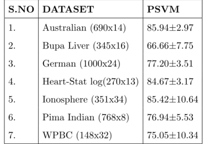
Table 2.6: Results of PSVM as a linear classifier for average 10-fold accuracy test with shuffling . S.NO DATASET PSVM 1. Australian (690x14) 85.94±2.97 2. Bupa Liver (345x16) 66.66±7.75 3. German (1000x24) 77.20±3.51 4. Heart-Stat log(270x13) 84.67±3.17 5. Ionosphere (351x34) 85.42±10.64 6. Pima Indian (768x8) 76.94±5.53 7. WPBC (148x32) 75.05±10.34

Table 2.7: Results of PSVM as a linear classifier for average 10-fold accuracy test without shuffling . S.NO DATASET PSVM 1. Australian (690x14) 85.94±5.68 2. Bupa Liver (345x16) 63.74±14.78 3. German (1000x24) 75.80±5.94 4. Heart-Stat log(270x13) 84.07±4.07 5. Ionosphere (351x34) 85.42±10.64 6. Pima Indian (768x8) 76.94±5.53 7. WPBC (148x32) 75.05±10.34

(32)

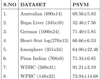
Table 2.8: Results of average 10-fold accuracy test using nonlinear kernel without shuffling . S.NO DATASET PSVM 1. Australian (690x14) 69.56±5.83 2. Bupa Liver (345x16) 52.46±7.56 3. German (1000x24) 71.40±5.85 4. Heart-Stat log(270x13) 66.66±6.53 5. Ionosphere (351x34) 64.00±22.46 6. Pima Indian (768x8) 71.34±6.85 7. WDBC (569x31) 91.21±3.19 8. WPBC (148x32) 73.94±14.68

Table 2.9: Results of PSVM for average 10-fold accuracy test using nonlinear kernel with shuffling . S.NO DATASET PSVM 1. Australian (690x14) 69.56±5.83 2. Bupa Liver (345x16) 52.46±7.56 3. German (1000x24) 71.40±5.85 4. Heart-Stat log(270x13) 66.66±6.53 5. Ionosphere (351x34) 64.00±22.46 6. Pima Indian (768x8) 71.34±6.85 7. WDBC (569x31) 91.21±3.19 8. WPBC (148x32) 73.94±14.68

(33)

2.6 Conclusion Introduction to SVM

2.6 Conclusion

As the size of the patterns increases, the training time increases and also the compu-tational complexity increases for SVM. In order to overcome the drawbacks of SVM, proximal support vector machine (PSVM) was developed. The classification accuracy of the PSVM is comparable to standard SVM but the computational complexity of PSVM is less than SVM. The training time required by PSVM is less compared to large training time in case of standard SVM.

(34)

2.7 References Introduction to SVM

2.7 References

[1] C. Cortes and V. N. Vapnik, “Support Vector Networks,”Machine Learning , vol. 20, pp. 273-297, 1995.

[2] C. J. C. Burges, “A Tutorial on Support Vector Machines for Pattern Recogni-tion,” Data Mining Knowledge Discovery, vol. 2, pp. 1-43, 1998.

[3] S. Haykin, Neural Networks- A Comprehensive Foundation, second ed., Pearson Education, 2006.

[4] S. R. Gunn, “Support Vector Machines for Classification and Regression,” tech-nical report, School of Electronics and Computer Science, Univ. of Southampton, Southampton, U.K., 1998, http://www.isis.ecs.soton.ac.uk/resources/ svminfo/.

[5] V. Vapnik, The Nature of Statistical Learning Theory , second ed. New York: Springer, 2000.

[6] S. R. Gunn, M. Brown, and K. M. Bossley. Network performance assessment for neurofuzzy data modelling. In X. Liu, P. Cohen, and M. Berthold, editors, Intelligent Data Analysis, volume 1208 of Lecture Notes in Computer Science, pages 313323, 1997.

[7] A. Basu, C. Watters, and M. Shepherd,“Support Vector Machines for Text Cat-egorization,” proc. IEEE-INNS-ENNS International joitn Conference on System Sciences, vol. 5, pp. 205-209, 2000.

[8] T. A. Shamim, M. Anwaruddin and H. A. Nagarajaram,“Support Vector Machine-based classification of protein folds using the structural properties of amino acid residues and amino acid residue pairs,”Bioinformatics, vol. 23, no. 24, pp. 3320-3327, 2007.

[9] B. Moghaddam and Ming-Hsuan Yang,“Learning Gender with Support Faces,” IEEE Trans. Pattern Anal. Mach. Intell., vol. 24, no. 5, pp. 707-711, May 2002. [10] T. Evgeniou, M. Pontil and T. Poggio. Regularization networks and support

(35)

2.7 References Introduction to SVM

[11] V. kecman,Learning and soft computing support vector machines neural networks and fuzzy logic machines, Massachusetts: The MIT Press. pp. 121-191.

[12] O. L. Mangasarian, E. W. Wild, “Multisurface proximal support vector classifica-tion via generalized eigenvalues,” IEEE Trans. Pattern Anal. Mach. Intell.,, vol. 28, no.1, pp. 69-74, Jan. 2006.

[13] J. A. K Suykens and J. Vandewalle, “Least squares support vector machine clas-sifiers,” Neural Process Lett, vol. 9, pp. 293-300, 1999.

[14] J. A. Suykens, T. Van Gestel, J. De Brabanter, B. De Moor and J. Vandewalle, Least Squares Support Vector Machines. Singapore: World Scientific publishing Co., 2002.

[15] G. Fung and O. L. Mangasarian, “Proximal Support Vector Machine Classifiers,” Proc. Knowledge Discovery and Data Mining, F. Provost and R. Srikant, eds., pp. 77-86, 2001, ftp://ftp.cs.wisc.edu/pub/dmi/tech-reports/01-02.ps.

[16] T. Evgeniou, M. Pontil and T. Poggio. Regularization networks and support vector machines. In A. Smola, P. Barlett, B. Scholkopf and D. Schuurmans, editors, Advances in Large Margin Classifiers, pages 171-203, Cambrige, MA, 2000. MIT Press.

(36)

Chapter 3 Datasets and Experimental setup

Datasets

(37)

3.1 Datasets Datasets and Experimental setup

3.1 Datasets

3.1.1 Cancer datasets

Cancer datasets are collected from Bioinformatics repository and UCI repository [1] for the purpose of our experiment.

Table 3.1: Cancer datasets used for results and comparison in our experiment.

Name No. of instances No. of genes

Colon 62 2000

Lung 22 56

AML-ALL 38 1000

Lymphoma 45 4026

Prostate 100 500

Description of cancer datasets:

(i) Colon cancer: It is known as colorectal cancer caused due to uncontrolled growth of cells in the colon or in an appendix or in the rectum.

(ii) Lung cancer: It is caused due to uncontrolled growth of cells in the tissues of the lung.

(iii) AML-ALL: AML is acute myeloid leukemia, it is caused due to uncontrolled growth of abnormal blood cells which are collected in the bone marrow and interfere with normal production of blood cells. ALL is acute lymphoblastic leukemia, it occurs due to accumulation of immature white blood cells which is reproducing continuously in bone marrow.

(iv) Lymphoma cancer: It is caused due to abnormal cell reproduction which may accumulate in one or more than one lymph nodes or in other lymph tissues.

(v) Prostate cancer: It is a cancer which occurs in the prostate gland. The prostate gland is found in male reproductive system.

(38)

3.1 Datasets Datasets and Experimental setup

3.1.2 Other datasets

These are some datasets collected from UCI repository [1] for experiment purpose.

Table 3.2: Details about other datasets used for results and comparison in our exper-iment.

Name No. of instances No. of genes Class ratio

Australian 690 14 307:383 Bupa Liver 345 16 200:145 German 1000 24 700:300 Heart-Stat log 270 13 150:120 Ionosphere 351 34 225:126 Pima Indian 768 8 500:268 WDBC 569 31 357:212 WPBC 148 32 151:27 Description of datasets:

(i) Australian: It contains the datasets for approval of Australian credit card.

(ii) Bupa liver: It contains the blood test results which are sensitive to liver disorder.

(iii) German: It contains the datasets for approval of German credit card.

(iv) Heart-Stat log: It contains datasets having information for heart disease.

(v) Ionosphere: It contains datasets having information of good or bad RADAR signal when it returns from the iononsphere.

(vi) Pima Indian: It contains datasets having information for detecting diabetes in Pima Indian heritage.

(vii) WDBC: It contains datasets containing digitized images taken with a fine needle aspirate of a breast mass.

(viii) WPBC: It contains datasets containing follow up information of digitized im-ages taken from a fine needle aspirate of a breast mass.

(39)

3.2 Experimental setup Datasets and Experimental setup

3.2 Experimental setup

All the datasets are collected from publicly available sources. All the numerical testing is done using MATLAB 7.6 Version [2] on Windows 7 operating system on a CPU with an i5 processor with a speed of 3.33 GHz and 4 GB RAM. Proposed method, SVM, LS-SVM and PSVM is tested for both linear and nonlinear kernel functions. In this thesis, SVM Tool Box [3], LS-SVM Tool Box [4] and PSVM Tool Box [5] is used for simulation purpose.

(40)

3.3 References Datasets and Experimental setup

3.3 References

[1] C. L. Blake, C. J. Merz, J. Vandewalle, “UCI Repository for Machine Learning Databases,” Department of Information and Computer Sciences, University of California, Irvine, 1998/http://www.ics.uci.edu/mlearn/MLRepository.html.

[2] MATLAB, Users Guide, The Math Works, Inc., 1994-2001/http://www.mathwor-ks.com.

[3] S. R. Gunn,SVM Matlab toolbox, http://www.isis.ecs.soton.ac.uk/resources/svm-info, 1998.

[4] LS-SVM Toolbox,version-1.5 advanced, http://www.esat. kuleuven.ac.be/sista/l-svmlab/.

[5] G. Fung, O. L. Mangasarian, SVM toolbox home page, http://www.cs.wisc.edu/d-mi/svm/psvm.

(41)

Chapter 4 LMS based linear proximal support

vector machine

LMS Based Linear PSVM

(42)

4.1 LMS Based Linear PSVM LMS based linear proximal support vector machine

4.1 LMS Based Linear PSVM

The objective of the proposed LMS-PSVM technique is to improve the performance of PSVM [1-3] classifier for the training patterns and to find the optimal hyperplane subjected to a constraint. The techniques used are based on least mean square (LMS) algorithm [4], [5]. LMS algorithm is an adaptive algorithm which includes iterative process that makes consecutive corrections to the weight vector in the direction which leads to minimization of error. The weight vector is expressed as the linear combina-tion of the previous and present input data weighted [4] by an analytical error. LMS algorithm is also called as stochastic gradient descent method [4], in which the filter is only adapted based on the error at the current time. The patterns to be classified are projected in space with the help of kernel functions. A linear kernel function is used for the data which is linearly separable in that space. When the data is not linearly separable in that space then they are projected to another high dimensional space with the help of nonlinear kernel function. In this chapter linear kernel LMS-PSVM is discussed and next chapter elaborates the nonlinear kernel LMS-PSVM. The detail of algorithm for the proposed method using linear kernel is as follows:

Step 1: The two planes which are to be constructed for classification is given below:

ωT_x₋_b _{= +1}

ωTx−b=−1 (4.1)

where ω is a weight vector defined in n-dimensional real space Rn_, _b _{is bias} term, which represents the relative position of the planes from the origin. Bias is defined in real dimensional space R. The given datasets are considered to be of dimension m×n, represented by A matrix. The hyperplanes in Eq. (4.1) are not bounding planes, but can be thought of as “proximal” planes, around which the datasets of each class are clustered. Y is a diagonal matrix of dimension m×m with +1 or -1 along its diagonal.

Step 2: To obtain the hyperplanes in Eq. (4.1), PSVM optimizes the cost function represented as:

(43)

minω,b,ξ 1₂[(ωTω+b2) +c||ξ||2]

s.t. Y(Aω−eb) +ξ =e (4.2)

where c is the regularization parameter and ξ is the slack variable or error variable. The first term of the objective function in Eq. (4.2) maximizes the margin between the two hyperplanes or minimizes the reciprocal of 2-norm distance between the two planes in the (ω, b) space of (n+ 1) dimensional real space. The objective function is subjected to a linear constraint, which states that the hyperplanes should be at a distance of 1 from the separat-ing hyperplane. The second term of objective function minimizes the error variable, thus attempting to minimize the misclassification. The separating plane, described below

ωTx−b= 0 (4.3)

lies midway between the two proximal hyperplanes (4.1) and separates datasets into class +1 and class -1. The solution of Eq. (4.1) is obtained by replac-ing the original problem by Lagrangian function. The Lagrange multiplier method solves the constrained optimization problem (4.2) by transforming it into a nonconstrained optimization problem (4.4). With this approach the optimization problem (4.2) can be expressed as

L(ω, b, ξ, ν) = 1 2||[ω, b]|| 2 + c 2||ξ|| 2₋ ν(Y(Aω−eb) +ξ−e) (4.4)

ν is the Lagrangian multiplier due to equality constraint. The Karush-Kuhn-Tucker (KKT) optimality conditions [5] for PSVM are obtained by equating the gradient of (4.4) to zero as follows:

∂L ∂ω = 0 →ω−A T_{Y ν} _{= 0}_, ∂L ∂b = 0 →b+e T_{Y ν} _{= 0}_, ∂L ∂ξ = 0 →cξ−ν = 0, ∂L ∂ν = 0 →Y(Aω−eb) +ξ−e= 0.                        (4.5)

(44)

The first three equations of (4.5) give the following expressions for ω,b, ξ in terms of the Lagrange multiplier ν.

ω =ATY ν b =−eTY ν ξ= ν c            (4.6)

Substituting values of (4.6) in the fourth expression of (4.5) allow us to obtain an expression of ν in terms of problem data A and Y as follows.

ν = (I c +Y(AA T ₊_eeT₎_Y₎−1_e = (I c +M M T₎−1_e _(4.7) where, M =Y[A −e] (4.8)

I is the identity matrix. Having ν from problem (4.9), one can obtain the optimal hyperplane (4.2) by equating value of ω, b, ξ from Eq. (4.6) in Eq. (4.2). The solution of (4.7) involves inversion of a large m×m matrix. We make use of the Sherman-Morrison-Woodbury formula [1] in order to reduce the inversion of a matrix to (n+ 1)×(n+ 1), which is smaller in dimension. Therefore the expression becomes

ν =c(I−M(I c +M

T_M₎−1_MT₎_e _(4.9)

Step 3: After constructing the hyperplane, LMS algorithm is used in order to enlarge the separating boundary, such that the data points of each class lies on the correct side of the hyperplane. The PSVM shown in Fig. 4.1 is for ideal case. Actual PSVM is shown in Fig. 4.2, some of the data points of each class are lying on the wrong side of the hyperplane, which is not present in the ideal case for PSVM. The datapoints lying on the wrong side of the hyperplane are assigned to matrix B and F. Matrix B contains the datapoints of class +1 having ωTx−b <0 and matrixF contains datapoints of class -1 having ωT_x ₋ _{b >} _0. _{Assume, the distance of these points from the separating} hyperplane as error is represented by

(45)

Figure 4.1: The ideal Proximal Support Vector Machine Classifier in the (ω, b)-space of Rn+1_{. The planes} _ωT_x₋_b ₌_±_{1 around which points of the sets +1 and -1 cluster} and which are pushed apart by the optimization problem (4.2).

Figure 4.2: The Proximal Support Vector Machine Classifier in the (ω, b)-space of Rn+1_{. The planes} _ωT_x₋_b ₌ _±_{1 around which points of the sets +1 and -1 cluster} and which are pushed apart by the optimization problem (4.2).

(46)

P1(j) = ωTB(j)−b (4.10)

P2(i) = ωTF(i)−b (4.11)

where j = 1,2, ..., N1, represents the number of data points of B and i = 1,2, ...., N2, represents the number of data points of F. Here, data points which fall on the wrong side of the hyperplane is taken. The weight vectors of these data points are modified at the training phase. LMS algorithm is developed for each data point which shows an error as follows:

ω(n+ 1) =ω(n)−ηB(j)E1(n) (4.12)

ω(n+ 1) =ω(n) +ηF(i)E2(n) (4.13)

where E1 and E2 are mean square error. Weight vector states the orientation of the hyperplane, here two different sign is used for two different classes. In order to make the datapoints fall on the correct side of the hyperplanes, the orientation of the hyperplanes should be changed. n and η represents the number of iterations and learning rate parameter respectively. The weight vector is updated till our mean square error is reduced to 0.00001.

Step 4: The weight vectors are stored and used for reduction of error due to datapoints lying inside the region of separation. In order to do this, those data points which fall inside the region of separation or shows misclassification is collected. The error for these data points [2] can be defined as E =y(i)−P(i), where i = 1,2, ....Ne. Ne is the number of the data points that make error, y(i) is the desired output andP is the distance of the data point from the separating hyperplane that are causing errors. The weight updating is done using the following equation:

ω(n+ 1) =ω(n)−ηG(j)E11(n) (4.14)

ω(n+ 1) =ω(n) +ηH(i)E22(n) (4.15)

where E11 and E22 represents the mean square error due to class +1 and -1 data and Matrix G and H contain data points of +1 and -1 which are

(47)

Figure 4.3: The proposed lms based proximal support vector machine classifier, after training the datasets lie outside the margin and on the correct side of the hyperplane.

lying inside the region of separation. The weight is updated till the mean square error is reduced to 0.00001. Fig. 4.3 represents the LMS-PSVM, where datasets lie on the correct side of the hyperplane and outside the margin. The updated weight vector was stored at the time of training phase and is used for testing purposes with the help of below function [4]:

ωTx−b          >0, then x∈+1, <0, then x∈ −1, = 0, then x∈+1 or x∈ −1. (4.16)

(48)

4.2 Experimental Results LMS based linear proximal support vector machine

4.2 Experimental Results

Table 4.1: Results of average 10-fold accuracy test using linear kernel without shuffling

.

S.NO DATASET SVM LS-SVM PSVM LMS BASED LINEAR PSVM

1. Colon (62x2000) 36.19±22.22 83.57±10.56 85.47±15.70 85.47±8.93

2. Lung (22x56) 43.33±47.25 41.66±30.95 41.66±38.18 58.33±30.95

3. ALL-AML (100x500) 72.50±42.50 90.00±16.58 84.16±17.26 95.00±10.00

4. Prostate (38x1000) 44.00±9.16 72.00±11.66 81.00±7.00 84.00±12.00

Table 4.2: Results of average 10-fold accuracy test using linear kernel with shuffling

.

S.NO DATASET SVM LS-SVM PSVM LMS BASED LINEAR PSVM

1. Colon (62x2000) 35.23±19.71 77.14±17.20 77.61±10.33 84.28±13.39

2. Lung (22x56) 40.00±30.91 38.33±37.30 40.00±30.91 56.66±22.60

3. ALL-AML (100x500) 71.66±13.54 94.16±11.81 87.50±16.77 95.00±10.00

(49)

4.2 Experimental Results LMS based linear proximal support vector machine

Table 4.3: Results of average 10-fold accuracy test using linear kernel with shuffling

.

S.NO DATASET SVM PSVM LMS BASED

LINEAR PSVM 1. Australian (690x14) 45.45±3.62 85.94±2.97 86.08±4.45 2. Bupa Liver (345x16) 57.95±23.20 66.66±7.75 69.63±7.08 3. German (1000x24) 30.00±4.64 77.20±3.51 78.00±5.54 4. Heart-Stat log(270x13) 44.44±5.73 84.67±3.17 85.18±3.70 5. Ionosphere (351x34) 64.00±21.31 85.42±10.64 86.92±4.51 6. Pima Indian (768x8) 34.91±7.35 76.94±5.53 77.58±3.69 7. WPBC (148x32) 24.38±14.60 75.05±10.34 76.28±2.29

Table 4.4: Results of average 10-fold accuracy test using linear kernel without shuffling

.

LINEAR PSVM 1. Australian (690x14) 44.49±2.67 85.94±5.68 86.52±4.35 2. Bupa Liver (345x16) 57.95±23.20 63.74±14.78 64.89±13.85 3. German (1000x24) 30.00±4.64 75.80±5.94 76.20±5.43 4. Heart-Stat log(270x13) 44.44±5.73 84.07±4.07 84.81±2.59 5. Ionosphere (351x34) 64.00±21.31 85.42±10.64 85.42±10.64 6. Pima Indian (768x8) 34.91±7.35 76.94±5.53 77.02±5.35 7. WPBC (148x32) 24.38±14.60 75.05±10.34 75.61±14.60

(50)

4.3 Conclusion LMS based linear proximal support vector machine

4.3 Conclusion

The result shows that the proposed method for linear classifier is better as compared to standard SVM, LS-SVM and PSVM for cancer datasets. The performance of proposed method for linear classifier for UCI repository datasets is better from SVM and PSVM. The experiment is performed on all the 5 cancer datasets from Table 2.1. Out of 5 datasets linear classifier shows better result for 4 datasets. Better accuracy is represented in bold letter. In case of UCI repository, out of 8 datasets linear classifer performs better for 7 datasets. Two sets of experiments are performed, in first set the sequence of the datasets is kept as it is but in the second set the dataset is randomized or shuffled for the training purpose. Table 4.1 and Table 4.2 represent the comparison and the result of cancer datasets with and without shuffling using standard SVM, LS-SVM, PSVM and LMS-PSVM as a linear classifier. Table 4.3 and Table 4.4 represent the comparison and the result of UCI repository datasets with and without shuffling using standard SVM, PSVM and LMS-PSVM as a linear classifier.

(51)

4.4 References LMS based linear proximal support vector machine

4.4 References

[2] S. Ghorai, S. J. Hossain, A. Mukherjee and P. K. Dutta, “Newtons method for nonparallel plane proximal classifier with unity,” Signal Process, vol. 90, pp. 93-104, 2010.

[3] S. Ghorai, A. Mukherjee and P. K. Dutta, “Nonparallel plane proximal classifier,” Signal Process, vol. 89, pp. 510-522, 2009.

[5] S. Ari, K. Hembram, G. Saha, “Detection of cardiac abnormality from PCG signal using LMS based least square SVM classifier,”Expert Syst Appl,vol. 37, pp. 8019-8026, 2010.

(52)

Chapter 5 LMS based nonlinear proximal

support vector machine

LMS Based Nonlinear PSVM

(53)

5.1 LMS-Nonlinear PSVM LMS based nonlinear proximal support vector machine

5.1 LMS-Nonlinear PSVM

In this chapter formulation to nonlinear classifiers by applying kernel trick to max-imum margin hyperplanes is discussed. The resulting algorithm is similar to formal but here every dot product is replaced by a nonlinear kernel function [1-3]. This allows the algorithm to fit the maximum margin hyperplane in a higher dimensional feature space (transformed feature space). The transformation may be nonlinear; thus though the classifier is a hyperplane in the high-dimensional feature space, it may be nonlinear in the original input space. In our work, we have used Gaussian radial basis function [4-6] as a kernel function for the nonlinear case. It nonlinearly maps patterns into a higher dimensional space, unlike the linear kernel used during linearly separable data classification. The Gaussian radial basis function has fewer numerical difficul-ties as compared to other kernel functions, but it is not suitable when the number of features is very large. In Gaussian radial basis function, instead of classifying data according to their attributes, some datasets from any one class are chosen as centers for classification. Here, the chosen centers from any one class is denoted by ¯C. A matrix is our input or given dataset and µ = _2σ12. σ is variance, when larger value

of µ is chosen, variance becomes smaller and hence the kernel becomes more stricter and vice versa. The kernel function used in our case is given by:

K(A,C¯T) =exp−µP(Ai−C¯jT)2 (5.1)

Step 1: The nonlinear proximal classifier is obtained from modified equality con-strained optimization problem (4.2). The equality concon-strained optimization problem is modified by replacing the weight vector ω by its dual equivalent ω =ATY ν from (4.6), to obtain:

min(ν,b,ξ) 1₂[(νTν+b2) +c||ξ||2]

s.t. Y(AATY ν−eb) +ξ =e (5.2)

Above objective function minimizes weighted 2-norm sums of the problem variables (ν, b, ξ) instead of (ω, b, ξ).

(54)

min(ν,b,ξ)∈Rm+1+m 1

2[(ν

T_ν₊_b2_{) +}_c_||_ξ_||2_]

s.t. Y(K(A, AT)Y ν−eb) +ξ =e (5.3)

The Lagrangian function to solve (5.3) can be written as:

L(ν, b, ξ, v) = 1 2||[ν, b]

T_||2₊ c 2||ξ||

2₋_v₍_Y₍_{KY ν}₋_eb_{) +}_ξ₋_e₎ _(5.4)

whereK=K(A, AT_{) and}_v_{is the Lagrange multiplier associated with equality} constraint of (5.3). The gradient of the above Lagrangian function is equated to zero to give the following KKT optimality conditions:

ν−Y KTY v= 0 b+eTY v= 0 cξ−v = 0 Y(KY u−eb) +ξ =e                    (5.5)

From first three equation expressions for (u, b, ξ) is obtained in terms of the Lagrange multiplier v:

ν =Y KTY v, b=−eTY v, c= v

ξ (5.6)

On substituting the above equations in the last equation of (5.5), following expression is obtained:

v = (I_c +Y(KKT ₊_eeT₎_Y₎−1_e

= (I

c +N N

T₎−1_e _(5.7)

where N is defined as:

N =Y[K −e] (5.8)

In nonlinear kernels, the Sherman-Morrison-Woodbury formula [4] is not re-quired because the kernel matrix K=K(A, AT_{) is a square matrix of} dimen-sion m×m, so the inversion takes place in high dimension. To reduce the m×m dimensionality of the kernel matrix reduced kernel techniques [7] can be used, so that the large dimensionality kernel matrix is reduced to a smaller

(55)

dimensionality kernel matrix. On using reduced kernel technique, kernel func-tion becomesK(A,D¯T_{) of dimension}_m_×_m0_{, where}_m0 _m_{and ¯}_D_{is a}_m0_×_n

random sub matrix of A. The nonlinear kernel generated surface is obtained by substituting ω=AT_{Y ν} _{from (4.6) into (4.3) as follows:}

ωxT −b= 0 ⇒xTATY ν−b = 0 (5.9)

If the linear kernel xT_AT _{is replaced by its corresponding kernel expression} K(xT_{, A}T_{), and substitute} _u _and _b _{from (5.6), to obtain:}

K(xT, AT)Y ν−b =K(xT, AT)Y Y K(A, AT)TY v+eTY v

= (K(xT, AT)K(A, AT)T +eT)Y v = 0 (5.10)

Step 3: The datapoints lying on the wrong side of the hyperplane are assigned to matrix Q and R. Matrix Q contains the datapoints of class +1 having (K(xT, AT)K(A, AT) +eT)Y v <0 and matrix R contains datapoints of class -1 having (K(xT_{, A}T₎_K₍_{A, A}T₎T ₊_eT₎_{Y v >}_{0. Assume, the distance of these} points from the separating hyperplane as an error. The equation is similar to linear LMS-PSVM but the matrix Q and R is replaced by its corresponding nonlinear kernel function, is represented by

P1(j) =ωTK(Q, QT)−b

P2(i) =ωTK(R, RT)−b (5.11)

wherej = 1,2, ...., N1, represents the number of data points ofK(Q, QT) and i = 1,2, ...., N2, represents the number of data points of K (R, RT). Those points which fall on the wrong side of the hyperplane is considered in this case. The weight vectors of these data points are modified at the training phase similarly as in linear LMS-PSVM. LMS algorithm developed for each data point which shows an error as follows:

ω(n+ 1) =ω(n)−ηK(Q, QT)E1(n) (5.12)

(56)

where E1 and E2 are mean square error. n and η represents the number of iterations and learning rate parameter. The weight is updated till the mean square error is reduced to 0.00001.

Step 4: Now the error due to data points lying inside the region of separation is corrected. The weight updating formula becomes:

ω(n+ 1) =ω(n)−ηK(U, UT)E11(n) (5.14)

ω(n+ 1) =ω(n) +ηK(V, VT)E22(n) (5.15)

Here E11 and E22 are mean square error due to class +1 and -1. The error is represented by E = y(i)−P(i), where i = 1,2, ...Ne. Ne is the number of datapoints that are causing errors, y(i) is the desired output and P is the distance of the data point from the separating hyperplane that make error. The weight is updated till the mean square error is reduced to 0.00001. The updated weight vector was stored at the time of training phase and is used for testing purposes with the help of below function [4]:

(K(xT, AT)K(A, AT)T +eT)Y v                      >0, then x∈+1 <0, then x∈ −1 = 0, then x∈+1 or x∈ −1 (5.16)

(57)

5.2 Experimental results LMS based nonlinear proximal support vector machine

5.2 Experimental results

Table 5.1: Results of cancer datasets for average 10-fold accuracy test using nonlinear kernel without shuffling

.

S.NO DATASET SVM LS-SVM PSVM LMS BASED NONLINEAR P-SVM 1. Colon (62x2000) 63.80±22.22 63.80±22.22 63.80±23.43 73.10±4.79 2. Lung (22x56) 43.33±47.25 56.66±41.63 41.66±50.18 61.66±31.47 3. ALL-AML (100x500) 27.50±42.50 2.50±7.50 72.50±44.79 72.50±27.51 4. Lymphoma (38x1000) 48.50±28.55 58.00±31.24 65.00±28.38 82.50±17.83

Table 5.2: Results of cancer datasets for average 10-fold accuracy test using nonlinear kernel with shuffling

.

S.NO DATASET SVM LS-SVM PSVM LMS BASED NONLINEAR P-SVM 1. Colon (62x2000) 64.76±11.20 64.28±14.86 65.00±27.33 65.47±17.75 2. Lung (22x56) 38.33±43.49 58.33±38.18 53.33±44.30 73.33±28.54 3. ALL-AML (100x500) 28.33±23.62 29.16±20.15 69.16±23.58 71.66±21.94 4. Lymphoma (38x1000) 48.50±19.88 63.00±18.33 66.50±21.35 73.50±28.09

(58)

Table 5.3: Results of UCI repository datasets for average 10-fold accuracy test using nonlinear kernel without shuffling

.

NONLINEAR P-SVM 1. Australian (690x14) 43.18±3.02 69.56±5.83 70.28 ±5.92 2. Bupa Liver (345x16) 57.95±23.20 52.46±7.56 67.52±5.67 3. German (1000x24) 30.00±4.64 71.40±5.85 72.20±6.01 4. Heart-Stat log(270x13) 44.44±5.73 66.66±6.53 68.14±6.34 5. Ionosphere (351x34) 64.00±21.31 64.00±22.46 64.00±22.46 6. Pima Indian (768x8) 34.91±7.35 71.34±6.85 74.99±7.31 7. WDBC (569x31) 68.46±17.14 91.21±3.19 91.74±2.97 8. WPBC (148x32) 24.38±14.60 73.94±14.68 75.05±15.18

Table 5.4: Results of UCI repository datasets for average 10-fold accuracy test using nonlinear kernel with shuffling

.

NONLINEAR P-SVM 1. Australian (690x14) 43.18±3.02 69.56±5.83 70.43 ±4.98 2. Bupa Liver (345x16) 57.95±23.20 52.46±7.56 64.89±6.45 3. German (1000x24) 30.00±4.64 71.40±5.85 73.10±4.43 4. Heart-Stat log(270x13) 44.44±5.73 66.66±6.53 68.14±7.24 5. Ionosphere (351x34) 64.00±21.31 64.00±22.46 64.42±8.89 6. Pima Indian (768x8) 34.91±7.35 71.34±6.85 74.08±4.37 7. WDBC (569x31) 68.46±17.14 91.21±3.19 92.24±2.37 8. WPBC (148x32) 24.38±14.60 73.94±14.68 76.65±5.38

(59)

Table 5.5: Time taken by the classifiers to train cancer datasets with reduced kernel matrix size . S.NO DATASET R.R=1 R.R=0.7 R.R=0.5 R.R=0.1 1. Australian (690x14) 228.53 212.23 198.21 181.90 2. Bupa Liver (345x16) 107.60 97.56 86.31 71.57 3. German (1000x24) 296.79 114.89 94.24 86.21 4. Heart-Stat log(270x13) 62.89 79.03 62.74 59.33 5. Ionosphere (351x34) 127.91 119.48 92.86 87.29 6. Pima Indian (768x8) 345.32 336.12 197.24 182.94 7. WDBC (569x31) 492.27 458.23 412.48 385.57 8. WPBC (148x32) 38.25 27.35 21.97 16.38

Table 5.6: Time taken by the classifiers to train UCI repository datasets with reduced kernel matrix size

. S.NO DATASET R.R=1 R.R=0.7 R.R=0.5 R.R=0.1 1. Colon (62x2000) 43.62 36.37 27.28 18.90 2. Lung (22x56) 10.34 10.28 8.43 7.90 3. ALL-AML (100x500) 17.90 17.89 14.26 12.57 4. Prostate (38x1000) 54.34 48.51 33.46 28.20 5. Lymphoma (38x1000) 32.54 31.23 23.09 13.14

(60)

5.3 Conclusion LMS based nonlinear proximal support vector machine

5.3 Conclusion

The result shows that the proposed method is better as compared to standard SVM, LS-SVM and PSVM for nonlinear classifier. The experiment is performed on all the 5 cancer datasets from Table 2.1. Out of 5 datasets nonlinear classifier shows better result for 4 datasets. The performance of proposed method for UCI repository datasets is better for 7 datasets out of 8 datasets. Better accuracy is represented in bold letter. Two sets of experiments are performed, in first set the sequence of the datasets is kept as it is but in the second set the dataset is randomized or shuffled for the training purpose. Table 5.1 and Table 5.2 represent the comparison and the result of cancer datasets with and without shuffling using standard SVM, LS-SVM, PSVM and LMS-PSVM as a nonlinear classifier. Table 5.3 and Table 5.4 represent the comparison and the result of UCI repository datasets with and without shuffling using standard SVM, PSVM and LMS-PSVM as a nonlinear classifier. Table 5.5 and Table 5.6 shows the result of reduced kernel matrix size. R.R is the reduction ratio, firstly R.R=1 means that the size of the matrix is not reduced. R.R=0.7 means that the size of the kernel matrix is reduced to 70% of the original matrix size. It is evaluated that as the size of the kernel matrix reduces the training time also reduces.

(61)

5.4 References LMS based nonlinear proximal support vector machine

5.4 References

[1] C. Cortes and V. N. Vapnik, “Support Vector Networks,”Machine Learning , vol. 20, pp. 273-297, 1995.

[2] C. J. C. Burges, “A Tutorial on Support Vector Machines for Pattern Recogni-tion,” Data Mining Knowledge Discovery, vol. 2, pp. 1-43, 1998.

[5] S. Ghorai, S. J. Hossain, A. Mukherjee and P. K. Dutta, “Newtons method for nonparallel plane proximal classifier with unity,” Signal Process, vol. 90, pp. 93-104, 2010.

[6] S. Ghorai, A. Mukherjee and P. K. Dutta, “Nonparallel plane proximal classifier,” Signal Process, vol. 89, pp. 510-522, 2009.

[7] Y.-J. Lee and O. L. Mangasarian, “RSVM: Reduced support vector machines,” Proc. First SIAM Int’l Conf. Data Mining,Apr. 2001, ftp://ftp.cs.wisc.edu/pub-/dmi/tech-reports/00-07.ps.

(62)

Chapter 6 Conclusion and future work

Testing and Comparison

Conclusion

(63)

6.1 Testing and Comparison Conclusion and future work

6.1 Testing and Comparison

The PSVM is implemented by using the PSVM Tool Box. 10-fold testing method is performed for the experiment. In 10-fold testing process, 90% of data is used for training purpose and 10% of data is used for testing purposes. This process is performed 10 times, so that each and every data is used for both testing and training purpose. In proposed LMS-PSVM, the number of iterations used for LMS algorithm is 100,000. The parameter η for an lms algorithm for all the datasets was preferred from the set 10−I_{, where} _i_{= 1}_,₂_,₃_,₄_...,_{20. On comparing the results of} LMS-PSVM with PSVM, it is found that the classification accuracy of LMS-PSVM is greater than PSVM in case of all except colon for linear classifier and ALL-AML for nonlinear classifier. On comparing the results of LMS-PSVM with PSVM, it is found that the classification accuracy of LMS-PSVM is greater than PSVM in case of all except ionosphere. LMS-PSVM classification efficiency is greater compared to standard SVM for all the datasets. In order to test the effectiveness of nonlinear kernel for LMS-PSVM, Gaussian kernel function is used to represent the datasets into high dimensional space. Due to strong convexity LMS-PSVM code is simpler than LS-SVM. Computation time in LMS-PSVM is reduced with the help of KKT optimality conditions and Sherman-Morrison-Woodbury formula. To compete with LMS-PSVM, more number training time is needed for SVM and it also requires more iterations. Large margin hyperplanes are obtained in case of LMS-PSVM, which in turn minimizes the generalization error. Minimum generalization error means that when a new set of data points with unknown class values arrive for the classification, the chances of occurring an error while predicting the class of the datapoints based on the hyperplane or learning classifier should be minimum. As lms algorithm is simple to implement, therefore the computational complexity of LMS-PSVM is not much higher than PSVM. LMS-PSVM not only works for a linear classifier, but also for a nonlinear classifier as well. In nonlinear case, the matrix A is replaced by K(A, AT) as input, and the pair (ω, b) is replaced by (ν, b), where ω = AT_{Y ν}_{. On shuffling,} it is seen that the performance increases for all the datasets. The training time of LMS-PSVM is not much greater than the training time of PSVM. For the reduced

Study on proximal support vector machine as a classifier

STUDY ON PROXIMAL

SUPPORT VECTOR MACHINE

AS A CLASSIFIER

STUDY ON PROXIMAL

SUPPORT VECTOR MACHINE

AS A CLASSIFIER

Dedicated to

Department of Electronics and Communication Engg

National Institute of Technology Rourkela

Rourkela-769008, Orissa, India.

Certificate

Acknowledgment

Abstract

Notations and terms

List of Figures

List of Tables

Contents

Chapter 1

Introduction

1.1

Motivation

1.2

Contribution

1.3

Organization of the thesis

Chapter 2

Introduction to SVM

2.1

Theoretical Background

2.2

Support Vector Machine (SVM)

2.2.1

Optimal Separating hyperplane

2.2.2

Architecture of SVM

2.2.3

Formulation of SVM

2.2.4

Kernel methods

2.3

LS-SVM

2.4

PSVM

2.5

Experimental Results

2.6

Conclusion

2.7

References

Chapter 3

Datasets and Experimental setup

3.1

Datasets

3.1.1

Cancer datasets

3.1.2

Other datasets

3.2

Experimental setup

3.3

References

Chapter 4

LMS based linear proximal support

vector machine

4.1

LMS Based Linear PSVM

4.2

Experimental Results

4.3

Conclusion

4.4

References

Chapter 5

LMS based nonlinear proximal

support vector machine

5.1

LMS-Nonlinear PSVM

5.2

Experimental results