School context and gender differences in mathematical performance among school graduates in Russia
Alexey Bessudnov1; Alexey Makarov2
Abstract: Gender differences in mathematical performance have received considerable scrutiny in the fields of sociology, economics, and psychology. We analyse a large data set of high school graduates who took a standardized mathematical test in Russia in 2011 (n=738,456) and find no substantial difference in mean test scores across boys and girls. However, boys have a greater variance of scores and are more numerous at the top of the distribution. We apply quantile regression to model the association between school characteristics and gender differences in test scores throughout the distribution of test scores. Male advantage in test scores, particularly at the top of the distribution, is concentrated in cities and in the schools with an advanced curriculum. In other high schools, especially in the countryside, gender differences in all parts of the
distribution are small. We suggest several mechanisms based on selection and school effects that account for our findings.
Key words: gender gap in mathematics; school effects; quantile regression; Russia
This is an Accepted Manuscript of an article published by Taylor & Francis Group in the International Studies in Sociology of Education, available online:
http://www.tandfonline.com/10.1080/09620214.2014.1000937.
DOI: 10.1080/09620214.2014.1000937
1 University of Exeter; National Research University Higher School of Economics 2 National Research University Higher School of Economics
1. Introduction
Gender differences in school test scores in general and in mathematical performance in particular have attracted considerable attention over the past several decades. Papers exploring this
problem have appeared in leading journals in sociology, psychology, and economics (Ellison and Swanson, 2010; Fryer and Levitt, 2010; Lindberg et al., 2010; Penner, 2008). This interest can be explained by several factors. Mathematical performance in school can affect career choice and is a good predictor of future earnings. Despite the continuing push for greater gender equality in the areas of labour market participation and education in Western countries, there remains a significant underrepresentation of women in science, technology, engineering and mathematics (STEM) sectors. The study of gender differences in math performance in school and on standardized tests helps explain to what extent they are related to gender inequality in STEM and, more generally, to what extent they can contribute to gender inequality in the labour market.
Most large-scale studies of the gender gap in mathematics are based on U.S. data. Further, cross-national studies (such as PISA and TIMSS) have much smaller samples and provide imprecise estimates of male and female distributions of the test scores at the country level. In this paper, we contribute to the literature by analysing a new data set containing the results of a standardized math test taken by all high school graduates in Russia in 2011 (n=738,456). The size of the data set allows us not only to look at the gender differences in means and variances, but to reliably model differences throughout the entire distribution of test scores using relative distribution methods and quantile regression. First, we compare test score distributions for boys and girls. Second, following the literature on the school-level determinants of the gender gap in
educational achievement, we model the association between school-level contextual factors (such as school type and location) and gender differences in the distribution of test scores.
The paper is structured as follows. Section 2 provides a review of the recent studies of gender differences in mathematical performance, both at the national and cross-national levels. Section 3 presents our research questions and describes the data and our statistical methods. Section 4.1 analyses gender differences in test score distributions in the data set. Section 4.2 explores school-level effects on the gender differences in test scores. Section 5 discusses the results substantively and concludes.
2. Literature review
There are several main themes running through the literature on the gender gap in mathematics. First, scholars try to establish whether there are indeed differences in mathematical achievement of men and women. Second, if these differences exist, are they better explained by biological or social factors? Third, a separate literature looks at the contextual (i.e. school- or neighbourhood-level) determinants of the gender differences in math.
The usual measure of gender differences in test scores is the effect size, d, that is the difference between mean values for men and women expressed in standard deviation units. Positive values of d show male advantage in test scores and negative values show female advantage. Absolute values of d below 0.2 can be roughly considered small, between 0.2 and 0.5 medium and above 0.5 large.
In an early meta-analysis Hyde et al. (1990) collected 100 studies published between 1963 and 1988 that reported 254 effect sizes based on the analysis of more than 3.1 million people (mainly in the USA). Averaged over all samples, d was found to be 0.15. When the study was limited to the samples of the general population only, d decreased to -0.05, slightly favouring women. These values suggested that gender differences in mean mathematical performance were very small. However, it was found that while there were no gender differences in mathematical problem solving in elementary and middle school, the gender gap favouring men emerged in high school and college.
Hedges and Nowell (1995) reported the results of a secondary data analysis of six large data sets collected in the USA between 1960 and 1992. They found slight advantage of men in
mathematical achievement (d ranged from 0.03 to 0.26). In a more recent study, Lindberg et al. (2010) conducted a meta-analysis of 242 studies published between 1990 and 2007 that involved about 1.3 million people. In this study, d was found to be 0.05. In a separate analysis of four large studies of American adolescents, they found d varying between -0.15 and 0.22.
Hyde et al. (2008) analysed mathematical test scores of about 7 million American school children from ten U.S. states and found d to be less than 0.1 in all grades (also see Hyde and Mertz, 2009). Contrary to the results of their previous study (Hyde et al., 1990), there was no evidence of a gender gap in mathematical performance emerging in higher grades. This finding partly contradicts earlier results of Leahey and Guo (2001). Based on data from the National
Longitudinal Study of Youth and the National Educational Longitudinal Study 1979, Leahey and Guo (2001) documented a faster rate of acceleration in math (especially in geometry) for boys, resulting in a slight gender gap favouring boys by 12th grade. Fryer and Levitt (2010) analysed the data from the Early Childhood Longitudinal Study Kindergarten Cohort 2003 (n=20,000) and found that upon entering kindergarten, boys and girls were about equal in math and reading scores. However, by the end of 5th grade, girls fell behind boys in mathematical test scores by roughly 0.2 standard deviations.
Overall, recent research shows that currently in the USA boys and girls are either equal or very close in mean mathematical performance. The evidence on whether a gender gap emerges in higher grades is contradictory, but, in any case, the gap is not large.
Another important consideration is whether focusing solely on mean differences in test scores by gender is masking important differences in the distributions of scores across boys and girls.. A standard measure of variability of test scores is variance ratio (VR), i.e. variance for men divided by variance for women. Variance ratios that are higher than one indicate greater male variability of test scores. Another way to measure variability is to look at the male/female ratio at different percentiles of the distribution of test scores.
It has long been argued that men show more variability than women in a number of
characteristics, including mathematical performance. Indeed, most research conducted in the USA and cross-nationally produced variance ratios for mathematical test scores that were higher than one, confirming the hypothesis of greater male variability. In the meta-analysis by Hyde et al. (2008) variance ratios ranged from 1.1 to 1.2. Hedges and Nowell (1995) reported similar results. Lindberg et al. (2010) reported the average VR of 1.08. Machin and Pekkarinen (2008) analysed cross-national data from PISA, TIMSS and PIRLS and documented greater variance for boys virtually in all countries (with minor exceptions), both for mathematics and reading. Strand et al. (2006) demonstrated greater male variability on the tests of verbal reasoning, non-verbal reasoning and quantitative reasoning, using data on 320,000 school pupils in the UK aged 11-12 years. Lohman and Lakin (2009) showed that these findings held for the USA as well and across birth cohorts. Ellison and Swanson (2010) looked at the gender composition of the participants of the American Mathematical Competitions, a selected sample of mathematically advanced American school children. While the proportions of boys and girls among all participants were not so different, the gender gap dramatically widened at the highest levels of achievement. At the 99.9 percentile the ratio of boys to girls was found to be 9 to 1, and all the top scorers were male.
Spelke (2005) presented some evidence against the hypothesis of greater male variability in math scores. However, she mostly discussed the potential gender bias in the SAT-M test. Later
analyses by Hyde et al. (2008), Lindberg et al. (2010) and Machin and Pekkarinen (2008) strongly support the hypothesis that boys have more variable test scores.
The central question of many studies of the gender gap in math achievement is whether the differences in the distributions of test scores are innate or rather have a social explanation. Disciplinary perspectives on this issue vary. Research in evolutionary psychology and cognitive studies demonstrated that hormonal sex differences do affect the way human brain functions in a very early age (Kimura, 2000; also see literature reviews in Buchmann et al., 2008; Penner, 2008). Arden and Plomin (2006) looked at the variability of intelligence among children of ages 2 to 10 and found greater male variability in test scores in all ages, except age two. Girls were overrepresented at the top of the distribution at age 2, 3 and 4, but by age 10 boys had higher mean and variance and were more numerous at the top of the distribution. These results do not necessarily prove that the gender differences in the distribution of intelligence are innate, but suggest that some gender differences, whether of hormonal nature or resulting from the process of socialization, emerge before the stage of formal education.
Sociology is largely informed by the social constructivist perspective that implies that biological sex differences are irrelevant for explaining gender differences in mathematical test scores and they should rather be explained by traditional gender stereotypes and norms that portray men as more capable for mathematics and science (for a review of possible mechanisms see Buchmann et al., 2008). Note that while these two perspectives are clearly different, they are not necessarily contradictory..Genetic influences may be activated in certain social environments (see Freese and Shostak, 2009), and gender differences in mathematical test scores may be affected by both biological and social factors.
As mathematical performance cannot be measured at birth, it is difficult to empirically separate innate and environmental reasons of gender differences in test scores. One of the approaches to this problem has been to study mathematical performance cross-nationally. It was argued that it is unlikely that genetic differences in cognition between genders vary by country. If we make this assumption, then all non-random, cross-national differences in d and variance ratios of test scores may be attributed to environmental---rather than innate---factors. The data used in
cross-national analysis come from three large intercross-national studies of performance of school children: PISA, TIMSS and PIRLS. The studies conducted with these data sets indicate that there are large cross-national differences in the size and sometimes in the direction of the gender gaps in
mathematics and reading.
Summarizing, the cross-national research of the gender gap in math shows the following picture. In older data sets from the 1990s, boys outperformed girls in most or even all countries (Baker and Jones, 1993; Marks, 2008; Penner, 2008). In more recent data sets, the evidence is more contradictory. PISA 2003 showed some average male advantage (Fryer and Levitt, 2010; Guiso et al., 2008), although it is fairly small (Else-Quest et al., 2010). In TIMSS 2003 and 2007 the average gender gap in math was virtually non-existent (Else-Quest et al., 2010; Kane and Mertz, 2012). In most countries, male-to-female variance ratios were greater than one, although there were some exceptions. In all data sets, there was significant cross-national variation in the size and direction of the gender gap. The attempts to explain this variation with some country-level predictors have so far been inconclusive. In some data sets there was a significant correlation between the gender gap and various measures of societal gender equality. However, these
correlations were absent in other data sets and, in any case, they cannot prove the causal effect of the level of societal gender equality on gender differences in test scores. Interestingly, a recent analysis also showed considerable cross-national variation in the gender differences in the attitudes to math among school children, with the gender gap favouring boys being larger in more affluent societies (Charles et al., 2014).
While the gender gap in math varies cross-nationally, it also varies across socio-economic contexts. Using data from the Beginning School Study conducted in Baltimore, Entwisle et al. (1994) showed that while mean performance of boys and girls was similar, the highest scoring boys usually coming from more affluent neighbourhoods outperformed the highest scoring girls. On the other hand, boys from disadvantaged neighbourhoods did worse compared to socially disadvantaged girls (also see Entwisle et al., 2007). This is consistent with the hypothesis of greater male variability. Entwisle et al. explained the emergence of this variability by greater susceptibility of boys to the effects of neighbourhood resources. Boys that came from socially disadvantaged neighbourhoods were likely to fall behind in their studies, while the effect on girls was less negative.
In a recent and more methodologically rigorous quasi-experimental study, Legewie and DiPrete (2012) found a similar effect with the data on socio-economic composition and reading test
scores of pupils in some elementary and upper-secondary schools in Berlin. Generally, girls did better in reading than boys. However, in schools with higher average socio-economic status (SES) of pupils’ families and better average performance, the gender gap favouring girls was considerably smaller (i.e., boys did relatively better). Legewie and DiPrete explained this effect by the differential impact of school environment on boys and girls. Schools with lower average SES had a male peer culture that promoted anti-school attitudes. This anti-school male culture was absent in schools with higher SES. Girls did not have the same anti-school peer culture in low-SES schools, and for them the effect of school environment on performance was weaker. Legewie and DiPrete (2014) further explored school effects on the gender differences in the probability of continuing education after high school in a STEM subject and found that the gender gap in college application for a STEM subject is associated with a high school’s curriculum in STEM and gender segregation of extracurricular activities. A recent study of Israeli schools (Cahan et al., 2014) also showed that school quality correlates with the gender gap in achievement: that is, in better schools boys tend to do comparatively better.
3. Research questions, data and methods
In this paper, we address two main research questions. First, we use a new data set of Russian high school students to assess the direction and the size of the gender gap in mathematics. This data allows us to expand on previous research that focuses either on the U.S. or cross-national data. Thus, we begin our exploration by asking the following question: are the results for Russian high school students different than previous research in the U.S. or cross-nationally?
Second, we look at the school-level correlates of the gender gap in math, such as school location, type and size. Following previous studies (Entwisle et al., 1994; Legewie and DiPrete, 2012), we hypothesize that the size of the gap may vary across schools with different characteristics. In particular, boys may do comparatively better in more academically oriented schools, with a more socially privileged student body.
Most previous studies looked at the gender differences in mean performance and variances only (Penner (2008) is an exception). Methodologically, we contribute to the literature by analysing the whole distribution of test scores and looking at the effects of gender and school-level characteristics throughout the distribution.
Our data come from the universal test in mathematics, taken by all high school graduates in Russia. In 2009, Russia introduced compulsory universal state examinations (USE, known in Russia by the acronym EGE) that high school pupils must take in order to graduate. The Russian language and mathematics are compulsory USE subjects, and more subjects are required to be able to apply to most universities. Universities have to accept USE as entrance examinations. The centrally administered USE replaced an old system of separate school and university exams, conducted locally.
The Russian school system has several tracks. First, there are several types of high schools that differ in terms of quality of education and socio-economic status of pupils. The majority of schools do not have any special status. Some schools, however, offer more advanced training in one or several subjects (such as mathematics, languages, etc.). Another type of schools, lycees
and gymnasiums usually have more advanced curricula in several subjects, better funding and are generally considered to be educational institutions of better quality. On the other hand, less academically successful pupils sometimes go to evening schools, although these are relatively rare. Apart from these main types, there are a smaller number of schools for children with disabilities, military schools, etc.
School education up to 9th grade (about age 14) is compulsory. After that pupils have a choice and can stay in school for another two years or leave and go to a vocational school. Staying in school for 10th and 11th grades is the academic track that usually (although not necessarily) leads to applying to a university. Vocational schools train for manual occupations (drivers, industrial workers, etc.) that usually take two years, or service industry jobs and lower
professional occupations (nurses, primary school teachers, hospitality workers, etc.) that as a rule takes four years. After completing a vocational school graduates can change their track and apply to universities or enter the labour market. The USE is mainly taken by 11th grade
graduates in the academic track, although a small number of students in vocational schools also take the exams in order to be able to continue their education in universities.
For the analysis in this paper we use the data set with the results of the USE in mathematics conducted in 2011. The data set contains valid records for the whole population of test takers (738,456 people). Most of students are 11th grade high schools pupils. Note that this is only part of the respective age cohort, as most pupils who left school after 9th grade and took the
1,178,500 (Rosstat, 2012). This is the same cohort of pupils who took the USE in 2011, so the proportion of USE takers in this cohort was roughly 0.63.
The fact that data are only available for a part of the population raises questions regarding potential selection bias. Nevertheless, these are the best data currently available for Russia, including the Russian portion of PISA, which is based on a much smaller sample.
The USE mathematical test in 2011 consisted of two parts. The first part had twelve problems; each correct answer was graded one point. The second part had six more complicated problems in the ascending order of difficulty, and students were required to present full solutions.
Problems in this part could be graded 2, 3 or 4 points. The exam covered the Russian high school curriculum for algebra and geometry. The maximum test score was 30. In order to standardize the scale for all subjects, the original score was rescaled by USE organizers to the 0 to 100 scale. In this paper, we use the original 30-point scale.
Apart from data on test scores and sex, the data set contains identifying variables for region, school and class, information on school location (urban vs. countryside) and school type.
Unfortunately, no other variables that characterize social background of test takers are available.
We measure gender differences in the USE math test using Cohen's d---that is, the difference in means in two groups divided by the pooled within-group standard deviation. The gender
difference in variability of test scores is given by variance ratio (VR) or, more precisely, the variance for boys divided by the variance for girls.
To compare the distributions of test scores for boys and girls beyond the differences in means and variances, we employ the concept of a relative distribution as suggested in Handcock and Morris (1999). We provide a brief description of this method in section 4.1.
The analysis of the school-level correlates of the gender gap in math applies OLS regression and quantile regression (Hao and Naiman, 2007) to model the effects of predictors not only on the mean, but the entire USE test score distribution. Details are given in section 4.2. Quantile
regression was estimated with the R package quantreg (Koenker, 2013). The relative distribution was estimated with the reldist package (Handcock, 2013).
4.1. Characteristics of the test score distribution
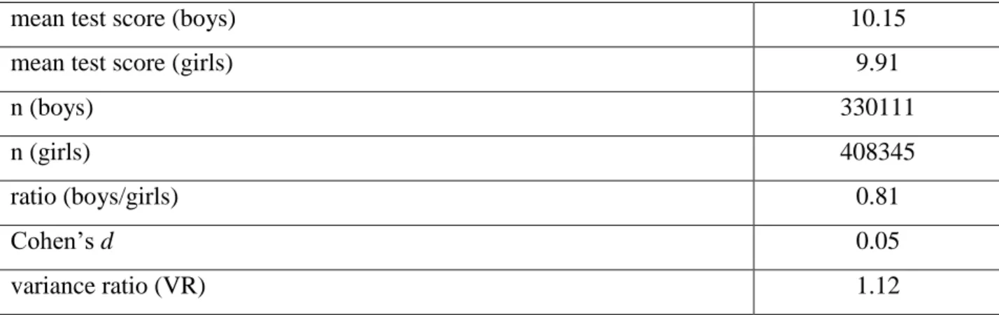
Table 1 presents some descriptive statistics, the effect size and variance ratio (VR) for the whole data set of USE test takers. The effect size, Cohen's d, is 0.05 that indicates that there is virtually no difference in mean test scores of boys and girls. VR is 1.12 showing somewhat greater variability of test scores for boys. Both findings are consistent with the results of the previous studies of the gender differences in mathematical achievement.3
Figure 1 plots test score distributions for boys and girls. To make a comparison of the two distributions beyond the differences in means and variances, we employ the concept of a relative distribution suggested in Handcock and Morris (1999). Figure 2 shows the probability mass function (pmf) for the relative distribution.
A relative distribution requires a reference group (in our case, boys) and a comparison group (girls). It shows what would be the rank of an observation taken from the comparison group in the reference group. For example, the relative distribution shows where in the male distribution would be a girl with the test score, say, 10. The pmf of the relative distribution is simply the ratio of pmfs for comparison and reference groups. Figure 2 thus shows the ratio of the heights of grey and black bars from Figure 1, plotted against the proportion of boys in the test score distribution. Figure 2 also presents a continuous approximation of the pmf.
If the two distributions were identical, the relative pmf would simply equal one throughout the reference distribution. However, as shown in the figure, in some parts of the distribution the relative density is clearly different from one. Girls are more likely than boys to be in the parts of the distribution where the relative mass is greater than one and less likely to be in the parts of the distribution where it is less than one. The plot shows that there is a higher chance for girls
(compared to boys) to score under 5 points (except zero points where boys are more represented) and from 11 to 15 points. The probability of scoring in the range between 6 and 10 points is slightly higher for boys. Also boys have a considerably higher probability of being in the top part
3We also compared the proportions of boys and girls who solved each of the 18 problems in the test. We
found the largest male advantage for the problems related to solid geometry (but not so much plane geometry). This is consistent with some previous studies that demonstrated a large male advantage for the problems that involve three-dimensional mental rotation (Halpern et al., 2007). We also found male advantage for a purely arithmetic problem and several most difficult problems in the test. There were two problems for which girls had some advantage over boys. One involved a system of equations, and the other was based on the geometric interpretation of the derivative.
of the distribution (starting from 16 points) and their advantage increases closer to the very top of the distribution. Note that only 3% of test takers get scores of 20 points and higher where male advantage is most evident.
As shown in Table 1, the ratio of the number of boys to the number of girls in the data set is 0.81. As the proportions of both sexes in the whole population in this age group are about equal, this indicates different rates of transition from 9th to 10th grade for boys and girls. If we assume that selection to 10th grade is at least partly based on academic ability, then, given that a larger proportion of boys leave school after 9th grade, the estimate of d in our sample is likely to be biased against girls. With our data it is not possible to estimate the strength of this bias.
4.2. School context and the gender gap in math
In this section, we model the association between the gender differences in math and a number of characteristics measured at the school level. In particular, we look at how the gender gap in math depends on the type of school and its location.
As shown above, mean performance of boys and girls is about equal, but there are other significant distributional differences. In particular, boys are more likely than girls to be among the top achievers (hence the higher variance for boys). To model the conditional median test score, while also modeling differences at various quantiles of the distribution, we apply quantile regression (Hao and Naiman, 2007).
We model the USE math test score as a function of gender, school type, school location, school and classroom size (the number of pupils in the same grade from the same school who took the exam, and the number of pupils from the same classroom), and the interaction effects between gender and all other predictors. The school and classroom size were standardized with the mean of zero and the standard deviation of one. We excluded from the analytical sample pupils from schools for children with disabilities and other non-standard types of schools, and also schools and classrooms with only one pupil, classrooms with more than 40 pupils and schools with more than 200 pupils taking the test (these are likely to be coding errors). We also excluded all
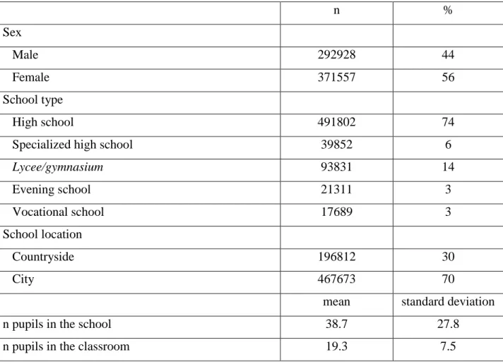
664,485 pupils (out of original 738,459)4. Descriptive statistics for the analytical sample is presented in Table 2.
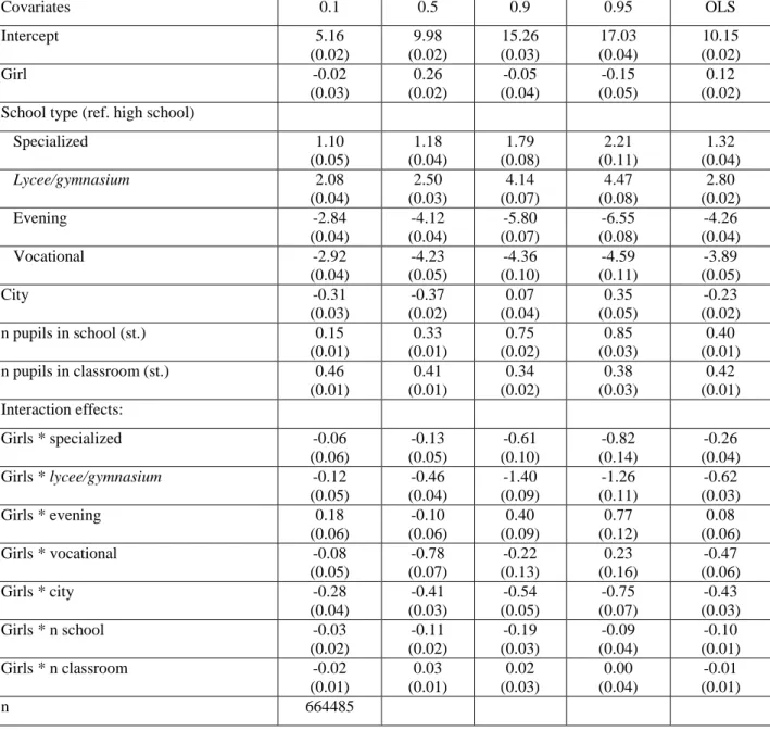
The results of the OLS and quantile regressions (estimated at 0.1, 0.5, 0.9 and 0.95 quantiles) are presented in Table 3. The results of quantile regressions (estimated at every 0.05 quantile) for selected effects (gender, school type, school location and interaction effects between gender and school type and location) are also graphically presented in Figure 3. As we are interested in the gender differences in test scores rather than predictors of test scores, we mainly interpret the effects for gender and the interaction effects between gender and other predictors.
To interpret the results, we look at the coefficients for regression equations presented in Table 3. We set the number of pupils in the school and the classroom at the mean level in our analytical sample (i.e., at zero, according to our coding). Then the predicted mean male test score in high schools in the countryside is simply 10.15 (the intercept in the OLS model). For girls at the same values of other predictors, the predicted test score in the OLS model is 10.27 (10.15+0.12). So, according to our model, in an average ordinary high school in the countryside girls slightly outperform boys.
Note, however, that the effect varies throughout the distribution. It is easy to see this from the plot for the main effect of gender in Figure 3. Taken by itself, it shows how the effect of female gender changes throughout the distribution for ordinary high schools in the countryside. At the 0.1 quantile, boys and girls perform about the same (the effect of gender is close to zero). In other words, the thresholds that separate the bottom 10% of girls and the bottom 10% of boys from the rest of the male and female distributions are about the same. At larger quantiles girls do somewhat better than boys, with the maximum female advantage at about the 0.6 quantile. Then female advantage diminishes, and the 0.95 quantile for girls is 0.15 smaller than for boys. Thus, in high schools in the countryside the results of both genders are similar throughout the test score distribution.
This effect changes once we move from the countryside to cities. In the OLS model the effect of female gender in ordinary high schools in cities is -0.31 (0.12-0.43), holding the number of
4We estimated the models without restricting the sample and the results were very similar. We also
estimated the OLS model with fixed effects for Russia's 83 regions. Compared to the model that did not control for region, this influenced some of the main effects (in particular, for school location), but the interaction effects that we are mainly interested in remained virtually unchanged. As estimating quantile regression models with fixed effects for regions was computationally difficult, we present the models without fixed effects.
pupils in the school and the classroom at their means. This is a weak effect, given the 30-point scale for test scores. However, the effect increases at the top of the distribution. As shown in the plots for the effects “girls” and “girls:city” in Figure 3, starting from the 0.8 quantile both curves on the plots go down, indicating larger female disadvantage at the top of the distribution. For example, the 0.95 quantile for girls in urban high schools is predicted to be 16.48 (conditional on the school and classroom size set at their mean level), while for boys it is 17.38, so that the difference is 0.9.
The main effects for school type establish a clear academic hierarchy. Lycees and gymnasiums
have the best results in the USE math test, followed by specialized schools and then ordinary high schools. Pupils from evening and vocational schools perform much worse.
The interaction effects between gender and school type show that the size of the gender gap in math depends on the type of school. For example, while in ordinary urban high schools the difference between male and female mean test scores is 0.31, in specialized schools it increases to 0.57 and in lycees and gymnasiums to 0.93. In evening schools the gender difference in means is 0.23 and in vocational schools it is 0.78. All these gender differences were calculated with the OLS coefficients presented in Table 3.
A much richer pattern emerges if we look at the top of the distribution. The visual analysis of plots “girls”, “girls:city”, “girls:s.specialized” and “girls:s.gymnasium” shows that at the top of the distribution all the curves go down, especially steeply for the interaction effect
“girls:s.gymnasium”5 .
As mentioned before, the difference between boys and girls at the 0.95 quantile in ordinary urban high schools is 0.9. However, in urban specialized schools it increases to 1.72 and in urban
lycees and gymnasiums to 2.16. These are substantial differences. They show that in schools with the highest level of performance and higher SES the top 10% of boys considerably outperform the top 10% of girls, even when the gender difference in mean scores is relatively small.
5 However, note a slight decrease in female disadvantage at the very top of the distribution (quantiles 0.9 and 0.95) in lycees and gymnasiums (see “girls:s.gymnasium”). It is difficult to say if this is a statistical artefact or a true reflection of some social process.
Evening and vocational schools show a different pattern. There is not much gender difference in test performance in any part of the distribution. At the 0.95 quantile in urban evening schools boys outperform girls by 0.12, and in urban vocational schools by 0.67.
In the countryside male advantage at the top of the distribution in specialized schools and lycees
and gymnasiums becomes somewhat smaller (compared to cities).
So far all these estimates were given for schools and classrooms of average size. As the coefficients in Table 3 suggest, there is virtually no effect of the school size on the gender differences in test scores. The OLS estimate of the interaction effect “girls: n school” is -0.1, indicating a very small female disadvantage in larger schools. The effect does not become larger at the top of the distribution. The effects of the classroom size on the gender gap in test results are very small and statistically not significant.
5. Discussion
Our analysis yields several conclusions. First, the gender difference for Russian high school students in mean mathematical test scores is negligible (d=0.05). However, boys show a greater variance of test scores than girls (VR=1.12). Both findings are consistent with the results
previously reported in the studies based on US and international data. Actually, the size of d that we find in Russia is exactly the same as in a recently published cross-national meta-analysis (Lindberg et al., 2010).
Gender equality in mean mathematical performance in the USA, Russia and a number of other countries disproves a popular myth that boys are on average more talented in math than girls. While some studies show that boys did better than girls in math in the 1990s (Marks, 2008; Penner, 2008), more recent data do not support this conclusion (Else-Quest et al., 2010; Kane and Mertz, 2012; Lindberg et al., 2010).However, greater male variability in mathematical test scores that we find with the Russian data is a more robust phenomenon reported in many other studies (Hedges and Nowell, 1995; Hyde et al., 2008; Machin and Pekkarinen, 2008).
Note that we only have data on about 60% of children in the age cohort, mainly those who completed 11th grade in high school. Children with lower academic performance often choose the vocational track after 9th grade. Most of them do not take the USE. The vocational track is
more common for boys than for girls, and the ratio of boys to girls in our data is about 8 to 10. Hence the results are probably biased against girls, and the size of this bias is unclear. Note, however, that this limitation is common for other research conducted in Russia on schoolchildren aged over 14. Besides, the gender-specific selection process of schoolchildren to 10th grade of high school must be seen not as mere “data limitation”, but as part of social reality that shapes their further chances in the educational system and in the labour market.
The analysis of the school-level correlates of the gender gap in test scores shows that the size and direction of the gender gap in math vary depending on the school type. In the schools of better quality with more advanced curricula (specialized schools, lycees and gymnasiums) boys perform at the USE math test better than girls, with the gender gap being larger at the top of the distribution. On the other hand, in ordinary high schools, evening and vocational schools gender differences either in means or at the top of the distribution are much smaller or even reversed.
Why is it so? One possible answer is simply selection. Children are not distributed randomly across different types of schools. Specialized schools, lycees and gymnasiums select more advanced pupils who also tend to come from families with higher socio-economic status. Some schools in this group only take pupils after primary school or even at a later stage when their abilities can be tested. If we assume that boys have a more dispersed distribution of ability before coming to school (either naturally or as a result of early-life environmental effects) and hence are more represented at the top of the distribution and better schools attract the best students, then it is not surprising that we only find substantial gender differences in certain types of schools.
However, it is doubtful that selection works perfectly and most children with better mathematical abilities get into schools with more advanced training. Cleary, the USE test score is not a good measure of pre-school mathematical abilities. Still, while the majority of pupils scoring at the USE test 25 and higher came from specialized schools and in particular lycees and gymnasiums, 33% of these pupils were from ordinary high schools.
Another explanation is the school effect. Legewie and DiPrete (2012) demonstrated a causal effect of the classroom's average socio-economic status on the gender gap in reading
performance. In classes with a higher average socio-economic status of students the advantage of girls in reading test scores was smaller (also see Cahan et al., 2014; Entwisle et al., 2007). The proposed mechanism for this effect was male peer culture that in the classes with lower average
SES discourages the investment of efforts into the learning process among boys. There may be a similar mechanism involved in our case, if boys in ordinary high schools have lower motivation for learning.
Another possible mechanism is gender stereotyping, either internalized or enforced by teachers and peers. In schools with advanced curricula in math the requirements for girls may be lower if they are considered to be naturally less able. As a result of gender stereotyping, girls themselves may feel less able for advanced mathematical training.
The gender differences in the USE math test scores also depend on school location. Controlling for the type of school, in urban schools male advantage is larger, with the effect being stronger at the top of the distribution. As with school type, selection can be a possible explanation. If more mathematically gifted children are more likely to live in cities and boys have a higher variance of abilities than girls before school, then we would expect a greater gender gap favouring boys in urban schools even without any additional effect of location.
Another explanation is an additional effect of school quality. School type is not the only indicator of school quality, and we would expect lycees and gymnasiums in cities to be better than in the countryside. There may also be a separate effect of location. Entwisle et al. (1994) suggest that boys' school performance can be affected by resources available in the
neighbourhood.
Given the cross-sectional design of our study, we are unable to separate convincingly the effects of selection and school context. The mechanisms we suggest cannot be tested with our data. Further studies are required to demonstrate if and to what extent there is a causal effect of school context on the gender gap in test performance and to clarify the social mechanisms involved. Note that the effects of selection and school context may be at work simultaneously and interact. If male variance of pre-school math abilities is greater than female and there are more boys at the top of the distribution, these differences may be further amplified in school as a result of
differential treatment of girls and boys by teachers and gender differences in mathematics self-concept.
References
Personality and Individual Differences, 41, 39-48.
Baker, D.P., and Jones, D.P. (1993). Creating gender equality: Cross-national gender stratification and mathematical performance. Sociology of Education, 66, 91-103.
Buchmann, C., DiPrete, T.A., & McDaniel, A. (2008). Gender inequalities in education. Annual Review of Sociology, 34, 319-337.
Cahan, S., Barneron, M., & Kassim, S. (2014). Gender differences in school achievement: a within-class perspective. International Studies in Sociology of Education, 24, 3-23.
Charles, M., Harr, B., Cech, E., & Hendley, A. (2014). Who likes math where? Gender
differences in eighth-graders’ attitudes around the world. International Studies in Sociology of Education, 24, 85-112.
Ellison, G., & Swanson, A. (2010). The gender gap in secondary school mathematics at high achievement levels: Evidence from the American mathematics competitions. Journal of Economic Perspectives, 24, 109-128.
Else-Quest, N.M., Hyde, J.S., & Linn, M.C. (2010). Cross-national patterns of gender differences in mathematics: A meta-analysis. Psychological Bulletin, 136, 103-127.
Entwisle, D.R., Alexander, K.L., & Olson, L.S. (1994). The gender gap in math: Its possible origins in neighborhood effects. American Sociological Review, 59, 822-838.
Entwisle, D.R., Alexander, K.L., & Olson, L.S. (2007). Early schooling: The handicap of being poor and male. Sociology of Education, 80, 114-138.
Freese, J. and Shostak, S. (2009). Genetics and social inquiry. Annual Review of Sociology 35: 107-128.
Fryer, R., & S. Levitt, S. 2010. An empirical analysis of the gender gap in mathematics.
American Economic Journal: Applied Economics, 2, 210-240.
Guiso, L., Monte, F., Sapienza, P., & Zingales, L. (2008). Culture, gender, and math. Science,
320, 1164-1165.
Halpern, D.F., Benbow, C.P., Geary, D.C., Gur, R.C., Hyde, J.S., & Gernsbacher, M.A. (2007). The science of sex differences in science and mathematics. Psychological Science in the Public Interest, 8, 1-51.
Handcock, M.S. (2013). Relative Distribution Methods. Los Angeles, CA. Version 1.6-2. Project home page at http://www.stat.ucla.edu/ handcock/RelDist.
Handcock, M.S., & Morris, M. (1999). Relative Distribution Methods in the Social Sciences. Springer.
Hao, L., & Naiman, D.Q. (2007). Quantile Regression. Thousand Oaks: Sage.
Hedges, L.V., & Nowell, A. (1995). Sex differences in mental test scores, variability, and numbers of high-scoring individuals. Science, 269, 41-45.
Hyde, J.S., Fennema, E., & Lamon, S.J. (1990). Gender differences in mathematics performance: a meta-analysis. Psychological Bulletin, 107, 139-155.
Hyde, J.S., Lindberg, S.M., Linn, M.C., Ellis, A.B., & Williams, C.C. (2008). Gender similarities characterize math performance. Science, 321, 494-495.
Hyde, J.S., & Mertz, J.E. (2009). Gender, culture, and mathematics performance. PNAS,106, 8801-8807.
Kane, J.M., & Mertz, J.E. (2012). Debunking myths about gender and mathematics performance.
Notices of the AMS, 59, 10–21.
Kimura, D. (2000). Sex and Cognition. Cambridge: MIT press.
Koenker, R. (2013). quantreg: Quantile Regression. R package version 4.96.
Leahey, E., & Guo, G. (2001). Gender differences in mathematical trajectories. Social Forces,
80, 713-732.
Legewie, J., & DiPrete, T.A. (2012). School context and the gender gap in educational achievement. American Sociological Review, 77, 463–485.
Legewie, J. & DiPrete, T.A. (2014). The high school environment and the gender gap in science and engineering. Sociology of Education 87(4): 259-280.
Lindberg, S.M., Hyde, J.S., Petersen, J.L., & Linn, M.C. (2010). New trends in gender and mathematics performance: A meta-analysis. Psychological Bulletin, 136, 1123.
Lohman, D.F. & Lakin, J.M. Consistencies in sex differences on the Cognitive Abilities Test across countries, grades, test forms, and cohorts. British Journal of Educational Psychology 79:
389-407.
Machin, S., & Pekkarinen, T. (2008). Global sex differences in test score variability. Science, 322, 1331-1332.
Marks, G.N. (2008). Accounting for the gender gaps in student performance in reading and mathematics: evidence from 31 countries. Oxford Review of Education, 34, 89-109.
Penner, A.M. (2008). Gender differences in extreme mathematical achievement: An international perspective on biological and social factors. American Journal of Sociology, 114, S138–S170.
Rosstat. (2012). Regions of Russia. Social and economic indicators 2012 [Regiony Rossii: Sotsialno-ekonomicheskie pokazateli 2012]. Moscow: Russian Statistical Office.
Spelke, E.S. (2005). Sex differences in intrinsic aptitude for mathematics and science? A critical review. American Psychologist, 60, 950–958.
Strand, S., Deary, I.J. and Smith, P. (2009). Sex differences in Cognitive Abilities Test scores: A UK national picture. British Journal of Educational Psychology 76: 463-480.
Tables
Table 1. Statistics for the whole sample
mean test score (boys) 10.15
mean test score (girls) 9.91
n (boys) 330111
n (girls) 408345
ratio (boys/girls) 0.81
Cohen’s d 0.05
Table 2. Descriptive statistics for the analytical sample n % Sex Male 292928 44 Female 371557 56 School type High school 491802 74
Specialized high school 39852 6
Lycee/gymnasium 93831 14 Evening school 21311 3 Vocational school 17689 3 School location Countryside 196812 30 City 467673 70
mean standard deviation
n pupils in the school 38.7 27.8
Table 3. OLS and quantile regressions of USE test scores on school- and classroom-level variables Covariates 0.1 0.5 0.9 0.95 OLS Intercept 5.16 (0.02) 9.98 (0.02) 15.26 (0.03) 17.03 (0.04) 10.15 (0.02) Girl -0.02 (0.03) 0.26 (0.02) -0.05 (0.04) -0.15 (0.05) 0.12 (0.02) School type (ref. high school)
Specialized 1.10 (0.05) 1.18 (0.04) 1.79 (0.08) 2.21 (0.11) 1.32 (0.04) Lycee/gymnasium 2.08 (0.04) 2.50 (0.03) 4.14 (0.07) 4.47 (0.08) 2.80 (0.02) Evening -2.84 (0.04) -4.12 (0.04) -5.80 (0.07) -6.55 (0.08) -4.26 (0.04) Vocational -2.92 (0.04) -4.23 (0.05) -4.36 (0.10) -4.59 (0.11) -3.89 (0.05) City -0.31 (0.03) -0.37 (0.02) 0.07 (0.04) 0.35 (0.05) -0.23 (0.02) n pupils in school (st.) 0.15 (0.01) 0.33 (0.01) 0.75 (0.02) 0.85 (0.03) 0.40 (0.01) n pupils in classroom (st.) 0.46 (0.01) 0.41 (0.01) 0.34 (0.02) 0.38 (0.03) 0.42 (0.01) Interaction effects: Girls * specialized -0.06 (0.06) -0.13 (0.05) -0.61 (0.10) -0.82 (0.14) -0.26 (0.04) Girls * lycee/gymnasium -0.12 (0.05) -0.46 (0.04) -1.40 (0.09) -1.26 (0.11) -0.62 (0.03) Girls * evening 0.18 (0.06) -0.10 (0.06) 0.40 (0.09) 0.77 (0.12) 0.08 (0.06) Girls * vocational -0.08 (0.05) -0.78 (0.07) -0.22 (0.13) 0.23 (0.16) -0.47 (0.06) Girls * city -0.28 (0.04) -0.41 (0.03) -0.54 (0.05) -0.75 (0.07) -0.43 (0.03) Girls * n school -0.03 (0.02) -0.11 (0.02) -0.19 (0.03) -0.09 (0.04) -0.10 (0.01) Girls * n classroom -0.02 (0.01) 0.03 (0.01) 0.02 (0.03) 0.00 (0.04) -0.01 (0.01) n 664485
Note: Standard errors (the kernel estimate of the sandwich method as provided in the quantreg R package) are in parentheses. Quantitative variables were standardized with the mean of zero and the standard deviation of one.
Figures
Figure 3. Results from quantile regression, estimated at every 0.05 percentile. The dots represent the estimates, the grey areas represent 95% confidence intervals. The light grey lines show the OLS estimates with 95% confidence intervals. The model includes all the predictors from Table 3.