The final publication is available at IOS Press throughhttp://dx.doi.org/10.3233/ICA-180567
Bayesian Learning of Models for Estimating
Uncertainty in Alert Systems: Application to Air
Traffic Conflict Avoidance
V. Schetinina,∗, L. Jakaiteaand W. Krzanowskib aSchool of Computer Science and Technology, University of Bedfordshire, UKbCollege of Engineering, Mathematics and Physical Sciences, University of Exeter, UK
Abstract.Alert systems detect critical events which can happen in the short term. Uncertainties in data and in the models used for detection cause alert errors. In the case of air traffic control systems such as Short-Term Conflict Alert (STCA), uncertainty increases errors in alerts of separation loss. Statistical methods that are based on analytical assumptions can provide biased estimates of uncertainties. More accurate analysis can be achieved by using Bayesian Model Averaging, which provides estimates of the posterior probability distribution of a prediction. We propose a new approach to estimate the prediction uncertainty, which is based on observations that the uncertainty can be quantified by variance of predicted outcomes. In our approach, predictions for which variances of posterior probabilities are above a given threshold are assigned to be uncertain. To verify our approach we calculate a probability of alert based on the extrapolation of closest point of approach. Using Heathrow airport flight data we found that alerts are often generated under different conditions, variations in which lead to alert detection errors. Achieving 82.1% accuracy of modelling the STCA system, which is a necessary condition for evaluating the uncertainty in prediction, we found that the proposed method is capable of reducing the uncertain component. Comparison with a bootstrap aggregation method has demonstrated a significant reduction of uncertainty in predictions. Realistic estimates of uncertainties will open up new approaches to improving the performance of alert systems.
Keywords.Alert systems, Uncertainty, Air traffic control, Bayesian Model Averaging, Monte Carlo methods
1. Introduction
Alert systems aim to predict patterns of critical events which can happen in the short term. The systems are designed to predict events which must be avoided un-der specified conditions on given data. In alert sys-tems the “ground truth” is unavailable and so has to be estimated within a simulated environment. This is ideally designed to realistically handle combina-tions of uncertainty factors involved in retrospective events, as well as in manoeuvring intents of pilots at-tempting to resolve a problem. The models are ex-pected to provide plausible prediction of alert events. In safety-critical applications, such as transport sys-tems [1,2,3], air traffic control [4,5] using simulation [6] and on-board Traffic Alert and Collision Avoid-ance Systems (TCAS) [7], civil engineering [8,9,10], and power plants [11,12,13], the estimation of accu-racy suffers from uncertainties existing in both the models and the data which are used for predictions.
Some alerts can be predicted less certainly than others in terms of intervals of predicted probabilities, see e.g. [1,14]. In this light, prediction intervals reflect
confidence of estimates within the probabilistic frame-work [15], providing important information about pos-sible risks in the form of posterior predictive distribu-tions.
In air-traffic control, uncertainties in the data and models affect predictions of the future positions of air-craft and increase the errors of detecting areas of a pos-sible conflict [16]. Errors of false positive type are de-fined asfalse alarmsornuisance, whilst errors of false negative type are defined aslateormissedalerts [17]. The uncertainty affects the accuracy of predicting the future positions of aircraft and increases errors in alerts of separation loss [18,19,20]. Short-Term Con-flict Alert (STCA) systems are used in airports, that have complex and intensive air traffic, to warn opera-tors and pilots when the distance between two aircraft is critically short in a given zone. Alerts generated by the STCA system warn about a possible conflict that is defined as loss ofsafe separationbetween two aircraft, see e.g. [21,22]. For prediction of possible conflicts, STCA systems use radar data provided by air traffic service. Distance and time to the Closest Point of Ap-proach (CPA) between the aircraft are the main factors
of collision risk, as defined in the pioneering research [23]. Factors such as wind, weather conditions, aircraft flight characteristics, unavoidable imprecision in oper-ations and manoeuvres, as well as impression of radar readings increase uncertainty in air traffic data, see e.g. [24,25,26].
In an intensive air traffic environment, it is criti-cally important to detect conflict alerts with the maxi-mum accuracy and reliability. Analysis of uncertainty factors, which affect the detection accuracy, therefore will bring new insights into the problem [27,28].
Uncertainty in aircraft conflict detection can be formulated within a probabilistic framework which has been shown to be capable of improving the opera-tional performance, as described in [29,30]. Other ap-proaches based on Monte Carlo simulation have been considered in [31,32].
The uncertainty in a prediction can be quite large when the data sets available for building the mod-els are small. To avoid this problem, it has been sug-gested that the performance should be reported in the form of a Bayesian confidence interval obtained by a method which provides conservative measures of the uncertainty [33]. Bayesian Model Averaging (BMA) methodology in theory provides the most accurate estimates of the predictive posterior distribution re-quired for calculating prediction intervals. BMA has been made computationally feasible by using Markov Chain Monte Carlo (MCMC) approximations [34].
Bayesian inference has been used for the learn-ing of flight trajectory patterns from real air traf-fic data [35,6,36]. The Bayesian MCMC method has been used to build a model of the STCA system from Heathrow air-traffic data, in order to analyse the uncertainty and determine factors that affect predic-tions [37]. Although the described method has demon-strated promising results in modelling the STCA sys-tem, patterns of predicted outcomes have not yet been estimated in terms of uncertainty. The analysis of such patterns is critically required in order to find areas in which STCA performance can be improved [17].
We observed that the Bayesian models can detect some patterns at a high uncertainty in the posterior predictive distribution. This happens because a large number of models generate contradictory outputs as a result of detecting two patterns, alert or normal. We can thus analyse models that vote for incorrect deci-sions in order to find factors that cause the uncertainty. Making patterns of interest transparent by using De-cision Tree (DT) models, Bayesian analysis provides new insights into areas of potential improvements of
prediction performance, as described in our previous work [38,39,40].
In this paper we describe a new Bayesian ap-proach to modelling alert systems on given data in order to (i) analyse the posterior predictive probabil-ity distribution of alert patterns and (ii) provide in-sights into the uncertainty of alert events. As outlined above, alert systems generate data which do not con-tain “ground truth”, and so modelling of the STCA system is required in order to identify patterns which are uncertain. Transparent modelling of an alert sys-tem therefore will bring insights into the uncertainty and conditions under which the uncertainty is raised.
In such circumstances, we assume that the uncer-tainty in alert patterns is characterised by the variance of the posterior predictive probability density. Predic-tions with a variance above a given threshold are iden-tified as uncertain, and so the number of such predic-tions is important for evaluating the uncertainty of an alert system. In our experiments the proposed method demonstrated a substantial reduction in the number of uncertain predictions by comparison with the boot-strap aggregation described in [41].
For the research in this paper, flight data were made available by the UK National Air Traffic Ser-vices [42]. The proposed method will be used on these data to demonstrate the ability (i) to recognise both certain and uncertain predictions, and (ii) to provide a significantly larger number of certain predictions by comparison with the bootstrap aggregation. Reliable analysis of patterns which increase probabilities of er-rors is critically important for finding new insights into areas in which alert systems can be improved when their performance cannot be straightforwardly estimated.
The rest of the paper is organised as follows. tion 2 provides related work on air-traffic control. Sec-tion 3 introduces the STCA problem and describes the flight data that are used in our experiments. The sim-ulation of alert probabilities is outlined in Section 4. The following Section 5 describes the methodology of Bayesian learning of DT models. The experiments with the proposed Bayesian method are described in Section 6, and the results are discussed in Section 7. Conclusions are presented in Section 8. Appendix A provides the geometrical extrapolation of the CPA, which is used for estimating alert probabilities.
2. Related Work
National authorities specify vertical and horizontal separation standards to maintain the safe navigation
of aircraft in controlled zones. These standards en-sure safe separation from the ground, other aircraft and from protected airspace [43]. When two aircraft in an airport environment are on a potential collision course, a conflict event occurs and the controller and pilots communicate a resolution action based on flight data. To insure that the minimum separation between the aircraft is maintained, the aircraft trajectory is pre-dicted so as to avoid the conflict zone. In this sec-tion we outline work related to predicsec-tion of conflict events.
2.1. Linear extrapolation in conflict alert and collision avoidance systems
In [27], the influence of radar surveillance perfor-mance on conflict detection and separation distances has been analysed by modelling a conflict alert system. It has been reported that reliable assessment of the dis-tances requires an advanced model which includes not only radar monitoring but also weather conditions un-der different failure scenarios.
Prediction of an aircrafts position in the future is based on extrapolation using the aircrafts flight data. The algorithm decides whether the aircraft pair will be in a critical zone within the time of arriving at the CPA. Based on such prediction, the TCAS [7] has signifi-cantly reduced the risk of collision [44,45]. There is a concern that false alarms decrease trust in the system and lead to ignorance of alerts [17].
Geometric-based predictions may be not suffi-ciently accurate when an aircraft does not behave as expected in the immediate future [46]. The uncertainty in a prediction is managed by increasing the minimum distance and threshold time to the CPA at which an alert will be detected. The alerts detected by using such a linear prediction model have to be adjusted so as to satisfy a trade-off between false and missed alert rates. It has been concluded that the probabilistic ap-proach directly determines the required balance. 2.2. Modelling with adjustable parameters
A Gaussian model is assumed, reflecting the uncer-tainty along aircraft flight paths [27]. The model pa-rameters are defined by an expected aircraft position and a variance determining a 95% position in the hor-izontal plane. Having adjusted the model parameters, a region is estimated for a given minimum separation, where a conflict is detected at a certain confidence in-terval.
A probabilistic conflict detection system pre-sented in [5] assumes a model simulating the errors of trajectory prediction, which is used to minimise missed and false alerts. In every conflict detection cy-cle, two trajectories are simulated for each aircraft: one trajectory is a baseline and the other, which contains prediction errors, is used for simulating conflict detec-tion and resoludetec-tion. In every conflict detecdetec-tion cycle, the baseline is used to determine whether the conflict detection is an error or not, and thus the performance in terms of false rates is estimated at a given level of prediction uncertainty.
Monte Carlo simulation of air traffic control has been presented as a realistic approach for risk assess-ment [31]. The simulation is based on models which represent interactions between components of a sys-tem. Assessment of the risk of a conflict between the aircraft is based on the results of Monte Carlo simu-lations. In practice, when limited flight data are avail-able, analysis of credibility intervals is required in or-der to realistically evaluate risks.
2.3. Probabilistic modelling of air traffic
Aircraft trajectory models, developed for evaluating the performance of air traffic alert systems, are limited in their ability to represent flight data [6,36]. The pro-posed methodology is based on a dynamic Bayesian network framework described in [47]. Experiments have demonstrated the efficiency of Bayesian models for evaluating risks of collisions.
The rigorous analysis of traffic control systems re-quires an accurate model of aircraft behaviour [6,36]. The feasibility of using a Markov decision process for analysis of an air-traffic alert system has been investi-gated in [26]. The different approaches for learning of traffic models from recorded flight data are evaluated. It has been found that one approach, which is based on prior trajectory patterns, performs well on simulated data, but it has difficulty with real-world data. The other approach uses Bayesian inference techniques to learn parameters of the traffic model employing a Markov model. This approach is made computa-tionally feasible with MCMC methods. The Bayesian models have been found to better represent the ob-served data.
An important consideration in air traffic alert sys-tems is how to evaluate uncertainty. Many collision avoidance systems use point estimates of the state instead of the full posterior state distribution. Deci-sion theoretical methods have been applied to colliDeci-sion avoidance, but the importance of state uncertainty has
required further investigation. A computationally effi-cient framework has been proposed in [20] for evaluat-ing the uncertainty. Examination of Monte Carlo simu-lations has demonstrated that the estimates of state un-certainty can significantly enhance safety of collision avoidance systems.
Advanced algorithmic techniques have been de-veloped for solving problems, which are caused by multiple sources of uncertainties in flight data, for col-lision avoidance [45]. These techniques employ proba-bilistic models capable of representing the uncertainty sources to optimise collision avoidance systems. Ex-periments on recorded flight data have confirmed a sig-nificant improvement in safety of collision avoidance systems.
Deterministic models of collision avoidance are not able to provide reliable estimates of collision risks. Probabilistic models are capable of representing the various sources of uncertainty. A model described in [48] has been developed within a probabilistic frame-work to handle the uncertainty in collision avoidance. 2.4. Ensemble methods
Ensemble methods, known from the literature also as bootstrap aggregation [49,50] and bagging predic-tors [41,51], aim to approximate the posterior pre-dictive distribution by sampling from data given for building the models. The ensemble methods signifi-cantly improve the accuracy of prediction under cer-tain conditions. A bagging method known as Random Forests (RF) [52] has provided substantial gains in ac-curacy, using such models as classification and regres-sion trees.
The ensemble methods have improved the predic-tion accuracy although estimapredic-tion of predictive distri-butions requires additional efforts to achieve condi-tions under which the prediccondi-tions are asymptotically normal, and the confidence intervals can accompany predictions [53]. The variability of predictions made by the bagging methods and RF has been also esti-mated in the form of standard errors [14]. In [54], the uncertainty has been defined as the variation in the ensemble of models, which quantifies the “disagree-ment” between the model outcomes.
2.5. Bayesian averaging over DT models
The use of DT models within the Bayesian learn-ing framework makes probabilistic inference trans-parent and capable of providing insights into factors that cause uncertainty in predictions [55,56,57]. DT
models are defined as hierarchical structures of split-ting and terminal nodes which recursively split data [58,59]. Tree-like models have been efficient for fail-ure analysis and outcome prediction in engineering ap-plications, see e.g. [60,61].
The Bayesian method represents a prediction model as a Markov chain having transition states. The current state is dependent on the previous state. Un-der certain conditions the Markov chain achieves sta-tionarity. These properties permit the generation of a large sample of model parameters, which is required to achieve the accurate approximation of predictive pos-terior density. By contrast, RF is based on the random subsampling from data and on random selection of predictors. This strategy can simulate the uncertainty in the data, but not in the model parameters, as we discussed in [62,63].
3. STCA Problem and Data
Air traffic control systems are primarily based on ge-ometric extrapolation of the minimal distance and ar-rival time at the CPA for an aircraft pair [46,44,5]. In our study we use this method to map the distances and times, which were estimated from the given flight data, onto alert probabilities that are required for evaluating the prediction accuracy.
3.1. Representation of flight data
The primary flight data are received from radar in-cluded in airport traffic control system. The received information is updated in each radar cycle. Flight data include radar positions of aircraft in the 3-dimension system of coordinatesx,yandz. The coordinatesxand y define the position of an aircraft in the xy lateral plane. The coordinatesxandyare relative to the radar position, and the coordinatezis altitude.
Fig. 1 shows the traces of an aircraft pair in coor-dinatesx,y, andz. The alert cycles here are marked by the filled (in Red) circles, while the normal cycles are shown blank. The starting positions of the aircraft are indicated by the numbers 1 and 2.
We can see that after the 20th radar cycle the sys-tem detects a series of 6 alarm cycles. Having been alerted, the pilot of aircraft 2 has undertaken an im-mediate manoeuvre to avoid a dangerous loss of sepa-ration with aircraft 1. During the alert cycles, the dis-tance between the aircraft critically decreased from 2500 to 90. The projections of the aircraft trajectories (in Grey) in the xy plane show that the aircraft
ap-100 105 110 115 120 −120 −115 −110 1.1 1.2 1.3 1.4 1.5 ·104 1 2 X,nm Y,nm Z,ft Pair 11
Figure 1. A radar track with alert cycles (in Red). Start positions of aircraft are denoted by the numbers 1 and 2.
proached each other at least 5 cycles before the first alert. This means that an earlier alert would enable pi-lots and operators to plan a more safe and efficient ma-noeuvre.
In our experiments we used the flight data that represent traces of aircraft pairs with detected alerts. Each trace includes a sequence of radar cycles as de-scribed above. A cycle in the sequence represents the movement of the aircraft pair and can be either nor-mal or alert. These data are selected for modelling the STCA system within the Bayesian framework in or-der to estimate the accuracy and uncertainty of alert detection.
For modelling the following predictor variables were extracted from the data: (i) the distancesdx,dy,
anddzbetween aircraft 1 and 2 along the coordinates
x, y, andz, respectively, and (ii) the velocitiesVx,Vy
andVzof the aircraft.
The distance between aircraft 1 and 2 is important for alert detection in the airport environment when air-craft change positions in coordinatesx,yandzduring landing or taking off, so thatd=q(d2
x+d2y)s2+dz2,
wheresis the scale factor which is set in our research at the fixed value of 1.
Information about timesT1 andT2 in the lateral plane for the aircraft 1 and 2 is also included in the set of predictor variables. Table 1 lists all 12 variables along with their ranges, where the negative values re-flect the positions of aircraft in the radar coordinate system.
Table 1. Predictor variables and ranges
Variable Notation Min Max Units
x1 dx -48.11 51.70 nmi x2 dy -52.93 35.78 nmi x3 dz -10297 8760 ft x4 d 2.40 10297.06 ft x5 vx,1 -691 584 kn x6 vy,1 -806 473 kn x7 vz,1 -83.10 96.66 kn x8 vx,2 -444 599 kn x9 vy,2 -527 426 kn x10 vz,2 -95.05 11.53 kn x11 T1 0 9 s x12 T2 0 9 s
In our experiments we used 2,526 radar cycles that represent traces of 66 aircraft pairs that were land-ing or takland-ing off at Heathrow. These traces were se-lected because of approaching a critical distance, so that an average alert rate was 19.7%. The number of cycles in a trace was dependent on the aircraft veloci-ties and, on average, was around 40.
4. Simulation of Alert Probabilities
As discussed in Section 1, the “ground truth” in alert systems is not available, and probabilities of alerts have to be simulated in a given environment. In this section we describe how alert probabilities are calcu-lated within our approach by using geometrical extrap-olation of the CPA defined by distanceDand timeT, defined in [27,28]. Let a function fA(D,T)denote the extrapolated proximity between aircraft on a danger-ous course. The function fAallows us to estimate the
probability of alertPAfor each given cycle in the
tra-jectory. Note that this function does not handle other factors which determine aircraft trajectories, and so it cannot fully explain the behaviour of the STCA sys-tem on given flight data.
In our approach, the function fAis built from the
recorded flight tracks represented by the distancesD and timeTwhich are calculated for the CPA of aircraft at each cycle of the recorded tracks. The flight data include the STCA outcomes for normal (0) and alert (1) cycles. Alert probabilities PA are then calculated
from the function fA(D,T) for given D andT. The probabilitiesPAare used for testing the ability of an
in the predicted outcomes between two groups, certain and uncertain.
A system for alert predictions is designed to be able to estimate the uncertainty in the predictions within the probabilistic framework. This ability in our approach is evaluated on the recorded flight data by analysing deviations,σ, of the posterior probabilities
of alert.
Let us consider the flight data that includen cy-cles made available for modelling of an STCA system and an estimator capable of predicting the probability density and estimatingσi for each cyclei=1, . . . ,n.
Having divided the flight data into training and test data sets, we can design an ensemble estimator on the training data and then calculate the standard deviation
σifor all cycles included in the test data. We can then
consider a threshold deviation σ0 which divides the predictions made by the estimator into two groups: one withσi≤σ0and the other withσj>σ0,i∈I1,j∈I2, whereI1 andI2 are the indexes of cycles in the two groups, respectively. Theσ0is a threshold which lies between min({σi}n1)and max({σi}n1). The predictions
in the first group have a smallerσ than those in the
second group, and thus the uncertainties in the alert probabilities predicted for cycles assigned to the first group are smaller than those assigned to the second group.
We can then verify whether the difference be-tween the two groups of cycles, in terms of the extrap-olated alert probabilitiesPA, is significant for a given
thresholdσ0. If the difference is found to be significant for a thresholdσ0, we can then accept that predictions in groupI1are certain and, by contrast, predictions in groupI2are uncertain. In our experiments we found that the modelfA, built on the retrospective flight data,
explains 0.801±0.006 of STCA predictions within 3-fold cross-validation. Appendix A describes the details of the geometric extrapolation of aircraft trajectories.
5. Bayesian Averaging over Decision Tree Models
This section provides details of MCMC implementa-tion of Bayesian averaging over DT models. DTs are known as hierarchical models consisting of splitting and terminal nodes. DT models are said to be binary if the splitting nodes divide data points into two disjoint subsets. The terminal node assigns an input to one of the possible classes, the probability of which is dom-inant [58]. For interpretation purposes, the single DT which provides the Maximum a Posteriori probability could be selected from a set of DT models that were collected for averaging [64].
5.1. Markov chain Monte Carlo algorithm
Except for trivial cases the Bayesian methodology of averaging over DTs can be feasibly implemented with MCMC approximation. For the approximation, the pa-rameters, θ, of a DT candidate are drawn from the given proposal distributions. A candidate is accepted or rejected according to Bayes rule calculated on the given data D. Given the m-dimensional input vector x which represent the flight parameters described in Table 1, data D, and model parameters θ, the
pre-dictive posterior distribution p(y|x,D), y∈ {1,C},is obtained by combining the predictive posterior distri-bution p(y|x,θ,D)of parametersθ(i) conditioned on
dataD, whereCis the number of classes. Full details of this process are given in our previous work [37].
In practice, information about the posteriorp(θ|D)
is often limited. In such cases the MCMC approxima-tion is achieved with a Metropolis-Hastings sampler, which explores the posterior distribution by making random proposals, see e.g. [65,66].
When DT models are grown, their dimensional-ity (or number of nodes) varies. The Reversible Jump (RJ) extension of MCMC makes possible the approxi-mation over such models [67]. Given priors and a suf-ficient number of samples, the RJ MCMC technique explores the posterior distribution and takes samples of model parameters.
The exploration of DT models of variable size has been efficiently made by using the following moves:
Birth movesrandomly split the data points falling in one of the terminal nodes by a new splitting node with a variable and rule drawn from the corresponding priors.
Death movesrandomly pick a splitting node with two terminal nodes and assign it as a single terminal with the united data points.
Change-split moves randomly pick a splitting node and assign it a new splitting variable and rule drawn from the corresponding priors.
Change-rule moves randomly pick a splitting node and assign it a new rule drawn from a given prior. The first two moves lead to a change in the di-mensionality of parameters. The other moves explore the distribution within the current dimensionality. In particular, the change-split move makes “large” jumps which potentially increase the chance of sampling from a maximal posterior. By contrast, the change-rule move makes “local” jumps in order to explore the de-tails of an area of interest.
As the birth and death moves change the dimen-sionality, Bayes’ rule includes a ratio to achieve the
condition for reversibility of Markov Chain. Details of the algorithm are given in [37].
There are two phases of MCMC simulation for Bayesian learning of DT models. At the first, so-called burn-in, phase the MCMC explores the parameters of a DT model in order to find areas with a high likeli-hood on the given data set. At the second, so-called post burn-inphase, samples of a DT model are col-lected for BMA. The most accurate results of BMA are achieved when prior information on DT models is available [68,69].
Within the Bayesian method, the best accuracy of approximation of predictive density is achieved when samples collected during the post burn-in phase are di-verse. However, in practice the desired diversity of DT models cannot be achieved in reasonable computing time when prior information on the models is absent or incomplete [69].
In general, the likelihood distribution of the model can have multiple modes, which limits the ability of MCMC to explore the full posterior distribution, as described, e.g., in [34]. However, our research is not specifically focused on this problem. Instead we con-sider the limitations of MCMC sampling of DT mod-els, which are caused by their hierarchical structures, as discussed in [69]. These limitations lead to poor mixing of DT models because of excessive number of nodes in the grown DT models. Consequently, the ensemble of DT models collected during the MCMC sampling will underperform, as shown in our work [70].
5.2. RJ MCMC sampler
When the Metropolis-Hastings algorithm makes a birth move, a terminal node withndata points{x(i)}n1 is proposed to be a new splitting node with a variable j∼U(1,m)and a thresholdq0∼f(x), where f(x)is the distribution function of data{x(i)}ni. The function f(x)is required to set a prior on the birth move, as described in Section 5.1. As the knowledge off(x)for each splitting node is limited, a uniform prior,U(a,b), is used, where(a,b)is an interval in which a proposal q0is expected.
A change move, that is applied to a DT splitting node, redistributes the data points that fall into the downstream nodes, and therefore can produce a split-ting node in which one of two branches contains fewer data points thanpmin. This condition can be written as
min(n(le f ti) ,nright(i) )<pmin, (1)
wheren(le f ti) andn(righti) are the numbers of data points in the left and right branches of theith splitting node.
If the prior on the number of splitting nodes is given properly, most samples are expected to be drawn from the posterior that is related to areas of interest. If such a prior is unavailable, a DT model will grow ex-cessively and most of the samples will be drawn from posterior distributions that are calculated for oversized DT models. As a result, the estimates of the predictive distribution will be biased, see e.g. [69].
In practice, priors on DT structures are often un-available, and the MCMC sampler cannot efficiently control DT structures, which leads to poor mixing. However, the DT structure can be better controlled with a sweeping strategy of the MCMC approximation as proposed in [70]. The main idea behind this strategy is to assign the prior probability of splitting DT nodes dependent on the range of values within which the size of a new data partition will exceed 2pmin.
This prior is adapted to the range of a data parti-tion. The new splitting thresholdq0proposed for vari-able jand partitioniis drawn from a uniform distribu-tion:q0∼U(a,b), where(a,b)is the interval of vari-ablexjat nodei:a=min(xj)andb=max(xj).
When the change move is applied to a node that is close to the DT root, distributions of data points in its terminal nodes can be greatly changed, and one or more terminal nodes can contain fewer data points thanpmin. If there is one such node, this node is swept
from the DT and the move is counted as a death move. In cases when there is more than one such node, the move is deemed unavailable according to the MCMC strategy [70].
Our proposed MCMC strategy differs from that described in [70] in the following aspect. Making a birth or change move, the MCMC algorithm proposes a new parameterq0which is assigned within an inter-val(a,b). This interval is estimated from the data sam-ples{x(i)}n1that fall into the DT node assigned for the move. Thus the knowledge of(a,b)excludes assign-ing a proposal q0 outside of this interval. This strat-egy satisfies the condition for reversibility of a Markov Chain, which is needed in order to provide an equal probability of assigning the reverseq. As a result, the efficiency of MCMC, in terms of acceptance rate and details of exploring posterior parameters, is expected to be increased. The detailed exploration is critically important in order to achieve the model diversity re-quired for accurate approximation of the predictive density.
The next section outlines pseudocode of the pro-posed adaptive strategy.
5.3. Pseudocode of adaptive strategy
Algorithm 1 outlines the main steps of the adap-tive strategy of assigning proposals. The algorithm re-ceives data points{x(i)}n
1that are required to be split by a given node, as well aspminwhich defines the
min-imal number of data points allowed in a node’s branch. The change move is applied to a DT split node to up-date its current thresholdq. Having received the data points, the algorithm finds the interval (a,b) which is required to avoid the condition in Eq. 1. The data
{x(i)}n1are sorted into ascending order in line 3 in or-der to find an indexiof the current thresholdqin line 4. Indexes i1 and i2 are counted within the allowed range and thenxmin andxmax are assigned in lines 5
and 6. The parametersdefines the range of a uniform proposal distribution functiong(q0|q) =U(q−s,q+s)
within which a proposalq0is drawn in line 8.
Algorithm 1Changeq
1: Input:Data{x(i)}n1,pmin,q
2: procedureCHANGEq 3: Sortx(1)≤x(2)≤ ··· ≤x(n)
4: Findi:x(i−1)<q,x(i)≥q,i=2, . . . ,n 5: xmin=x(i1), wherei1=max(pmin,i−pmin)
6: xmax=x(i2), wherei2=min(i+pmin,n−pmin)
7: s=min(q−xmin,xmax−q)
8: Proposalq0∼U(q−s,q+s)
9: returnq0 10: end procedure
6. Experiments
In this section we describe experiments with the pro-posed Bayesian method on real STCA data. The aim of these experiments was to verify the ability of the proposed method to model outcomes of the STCA sys-tem with a reasonable accuracy. In our experiments we aim to find patterns which make uncertain contribution to the prediction. This is required for finding areas in which the accuracy of alert systems can be improved. 6.1. Experimental settings
In our experiments STCA probability is predicted for each cycle of an aircraft pair trajectory within the pro-posed Bayesian framework described in Section 5. The cycles are represented by the input variablesx1, . . . ,x12 described in Section 3.1. The Bayesian method
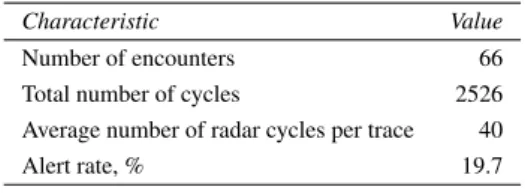
esti-Table 2. Flight Data statistics.
Characteristic Value
Number of encounters 66
Total number of cycles 2526 Average number of radar cycles per trace 40
Alert rate, % 19.7
mates a predictive probability density of an alert for a given cycle. Estimates of the probability density are then used for evaluating the uncertainty of the pre-diction. If the uncertainty in terms of deviation of the predictive probability density is high, the prediction is said to be “uncertain”, otherwise the prediction is said to be “certain”. For estimating predictive poste-rior densities, the Bayesian method employs DT mod-els built on the recorded flight data. DT modmod-els grown on these data have different sizes and so the Bayesian method uses RJ MCMC to handle variable dimen-sionality of model parameters. Reversible Jumps are made by the MCMC sampler outlined in Section 5 by proposing the parameter q0 for the moves which change dimensionality of the DT model. The proposed changes can be rejected or accepted. Eq. 1 defines a condition when DT node i is unavailable for a pro-posed move. Algorithm 1 outlines moves that are more likely to be accepted and thus the efficiency of the MCMC sampler will be improved. This condition de-fines when a DT node can further split the data into smaller subsets.
DT models outlined in Section 2 are used for STCA prediction as follows. The input variables which represent the flight data at a given cycle feed the DT models accepted by the MCMC algorithm. The av-erage over outcomes of these models is the predicted probability of alert at the given cycle. The model out-comes represent a predictive probability distribution of the alert, which is required in order to estimate the uncertainty in predictions. As discussed DT models are easy-to-interpret and for this purposes the Maxi-mum a Posterior model can be selected. An example of the interpretation of DT models for predicting alerts is provided in Section 6.4.
The experiments were run within 10-fold cross validation so that each fold contains 59 aircraft traces, which were selected for training, and the remaining 7 for testing the accuracy of alert detection. Table 2 summarises the information about the flight data, de-scribed in Section 3.1, which were used in our experi-ments.
An advantage of using DT models is that these models are applied “off-the shelf” as noted in [52], and so the BMA method does not require many settings, as discussed in [68,69].
The proposed Bayesian method was run with a uniform prior on DT models as there was no informa-tion about possible DT structures. The minimal num-ber pmin was set equal to 5. The proposal
probabili-ties for the birth, death, change-split and change-rules were set to 0.1, 0.1, 0.2, and 0.6, respectively. The first two probabilities, the birth and death moves set to 0.1, enabled the MCMC sampler to explore DT configu-rations with a reasonable intensity during the burn-in phase. Typically, larger DT configurations require more intensive proposals of the birth and death moves, see e.g. [37].
Setting the probability of the change-split to 0.2 enabled the MCMC algorithm to make the “large jumps” that increase a probability of exploring all ar-eas of interest and avoiding oversampling from arar-eas of local maxima. The remaining proposal probability of 0.6 is assigned to the change-rule to enable the sam-pler algorithm to explore details of the posterior dis-tribution of DT model parameters of a current config-uration. We found that with the given priors the above proposal probabilities provided the best performance of the Bayesian method with a reasonable efficiency of MCMC sampling, which is achieved when an ac-ceptance rate ranges between 0.25 and 0.7, according to [34].
The number of burn-in and samples was set to 100,000 in order to achieve a stationary Markov chain. In order to collect sufficient posterior samples to achieve a desired approximation accuracy, the number of post burn-in samples was set to be 10,000. Markov chains generate correlated samples, and so the gener-ated samples were decorrelgener-ated in order to obtain an i.i.d. sequence by drawing each 10th sample in the post burn-in phase. The proposal variance was set to 4.0 to achieve an acceptance rate of updating the Markov chain around 0.4, which is within the range of efficient MCMC sampling. With these settings, the Bayesian performance within the 10-fold cross-validation was 82.1%±σ, whereσ=5.1% is the standard deviation.
In the burn-in phase the Markov chain started with log a low likelihood value around -1000, converging to a higher value that oscillates around -175. In the post burnin phase the log likelihood oscillated between -200 and -150. The lower plots show that the average number of DT nodes was around 46.
6.2. Experimental settings for Random Forest RF, as an ensemble method discussed in Section 2, can approximate posterior predictive probability distribu-tions. In our experiments we applied this technique to the flight data with the following parameters. The number of DT models (or ensemble size) was 5,000. The bootstrap sampling rate (or fraction of input data to sample) was set to 0.7. The number of predictors to be randomly selected for DT splits was 10 out of the 12 described in Table 1. These parameters have en-abled the RF to achieve a highest prediction accuracy of 83.2% and so approximate a probability distribution of interest.
6.3. Analysis of uncertainty in alert predictions This section describes the experiments aimed at evalu-ating the uncertainty in STCA predictions on the flight data described in Section 3.1. The data are represented by the predictor variables that characterise the flight trajectories of aircraft pairs. The tracks were selected with alert cycles that were recorded nearest to a closet point of approaching. In the given airport environment the number of such tracks was very small. The total number of cycles was 2,526, and each cycle has a label A=1 (alert) or A=0 (normal). The experiments were run to compare the proposed Bayesian and existing RF methods in terms of accuracy of estimating the uncer-tainty of predictions made by the STCA system on the given flight data.
Let us consider track 2 shown on Fig. 5 and es-timate the posterior predictive probability densities of alert for each cycle by using the proposed (BDT) and existing RF methods. The related experimental set-tings were discussed in Sections 6.1 and 6.2. Fig. 5 shows this track including 42 cycles in which cycles 21 to 33 were detected as alert (shown in Red), and cycles before 22 and after 33 are normal.
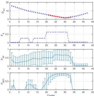
Fig. 2 shows the distances DXY between aircraft
pair A1 and A2 along with the extrapolated probabil-ities of alerts,PA, for cycles 1 to 42. The probabilities
PA increase from cycle 1, having a drop at cycle 11
as a result of change in flight direction of aircraft A2, shown on Fig. 5. Then between cycles 20 and 31 the probabilitiesPAreach a maximum around 0.67, whilst
the STCA system has predicted alert events between 21 and 33 cycles. We see that the estimations of PA
explain the alert events along the cycles, but impor-tant information about uncertainties in the predictions is absent.
RF as an ensemble method, discussed in Sec-tions 1 and 2, is capable of approximating the posterior probability densities, providing the predicted probabil-ities along with the ensemble variances which reflect the uncertainty in predictions. The predicted probabili-ties,PRF, and the ensemble standard deviation,σ, were calculated for the cycles 1 to 41 and shown as error bars on the third subplot of Fig. 2. Theσreflect the un-certainties in predicted probabilitiesPRF. We can see
that the values ofσremain large between cycles 1 and 20 in the absence of alerts as well as between cycles 21 and 34 in the presence of alerts. The values ofσ
decrease only after the last alert cycle 34. Thus the RF based estimator fails to indicate the relevant uncer-tainty level at cycles which precede the alerts.
The posterior probability densities of interest were calculated by the proposed BDT method and are shown in the fourth subplot of Fig. 2 as error bars. We see that the alert probabilitiesPBDT and the values of σ differ from those calculated by the RF estimator. Both the alert probabilitiesPBDT andσ at cycles 1 to
18 remain low, except cycles between 9 and 13 when the aircraft A2 has changed the flight direction. The probabilitiesPBDT increase to 0.9 during alert cycles
between 21 and 33. Thus in comparison with the RF estimator, the BDT provides more accurate informa-tion on the predicted alert probabilities and uncertain-ties. The RF estimator provides predictions variations of which are unreasonably large.
It is interesting to observe in Fig. 2 and Fig. 5 that at cycle 10 the aircraft A2 changed direction so that the distance of CPA was increased, thus decreasing the probability of conflict. The alert probabilitiesPRFand
PBDT predicted at this cycle are equal to 0.31.
How-ever, at the previous cycle 5 of these probabilities were PRF=0.23 andPBDT =0 with the σRF=0.363 and σBDT =0.05, respectively. This shows that the BDT
outcomes at cycles 5 and 10 are more realistic than the RF outcomes.
Table 3 shows the standard deviations σRF and σBDT calculated for the cyclesk=5,10, ...,35 along
with the alert probabilitiesPRF andPBDT and alert
la-belsA∈ {0,1}. It is interesting to note that cycle 20 is normal whilst the next cycle 21 is alert, but the RF estimator predicts the cycle 20 with PRF =0.5 and σRF=0.383, whilst the BDT givesPBDT =0.45 and σRF=0.451. Cycle 20 has A=0 and the BDT
out-come is more accurate than that provided by the RF. For the other cycles the values ofσBDT are
substan-tially smaller thanσRF.
The above results allow us to make the following observations:
Figure 2. DistancesDXYbetween aircraft pair A1 and A2 (subplot
1) along with the extrapolated probabilities of alertsPA(subplot 2)
over cycles 1 to 42. Posterior predictive probability densities of alert for cycles 1 to 42 estimated by the existing RF (subplot 3) and pro-posed BDT (subplot 4) methods.
Table 3. Standard deviationsσfor RF and BDT methods.
k σRF σBDT PRF PBDT A 5 0.363 0.005 0.23 0.00 0 10 0.352 0.275 0.31 0.31 0 15 0.435 0.005 0.45 0.00 0 20 0.383 0.451 0.50 0.47 0 25 0.310 0.148 0.67 0.91 1 30 0.295 0.100 0.67 0.94 1 35 0.129 0.006 0.05 0.01 0
(1) Variations in model outcomes included in an ensemble estimator reflect the ability of the estima-tor to approximate the posterior probability density of alert for a cycle.
(2) The standard deviation σ of the posterior probability density estimated for a cycle reflects the uncertainty in the prediction.
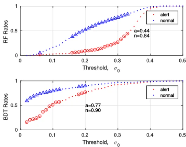
Given a threshold deviation σ0, we can find ra-tios of alert and normal cycles which are assigned by the RF and BDT estimators to the certain group. Fig 3 shows these ratios over the thresholdsσ0. The trian-gles and circles denote that the differences between the certain and uncertain groups are significant in terms of the extrapolated probabilitiesPA. The differences are
Figure 3. Ratios of alert (Red circles) and normal (Blue triangles) cycles assigned to the certain group by the RF and proposed BDT estimators:aandnare the ratios of alert and normal cycles, respec-tively.
verified with a 2-sample Kolmogorov-Smirnov test at a significance levelα<0.05.
The maximum rates of the certain alert and nor-mal cycles, which are obtained with the RF and BDT estimators, are aRF =0.44,nRF =0.84 and aBDT =
0.77,nBDT=0.90, respectively. The Wilcoxon signed
rank test shows that in comparison with RF the pro-posed BDT method provides a statistically significant increase,p<2·10−5, in the numbers of certain pre-dictions.
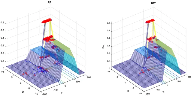
Cycles assigned to the uncertain group can be vi-sualised on a plane of distancesDand timeT of CPA, calculated for given flight data. The scattering of cy-cles which have been assigned to the uncertain group by the RF and BDT estimators is plotted in Fig. 4 on the right and left plots, respectively.
On these plots we can observe that the normal cycles (in Blue) are scattered more widely and inten-sively for the RF method than those assigned by the BDT method. The alert predictions (in Red) are also scattered more intensively for the RF method. This means that the RF method providing a comparable prediction accuracy tends to overestimate the uncer-tainty in both the alert and normal predictions. 6.4. Interpretation of alert patterns
Following [71,72], we would like to consider how models developed for alert predictions can be inter-preted. This section provides an example of using DT models for predicting patterns of interest. According to our approach Fig. 2 shows the probabilities of alerts for the RF and BDT methods. In this Figure we can
Table 4. A subtree predicting alert probability at cycle 2.
i vi qi p1 p2 xi 1 4 3543.75 0.00 1807.06 2 7 11.78 13.25 3 3 -1678.53 -1807.00 4 9 -247.36 0.00 273.00 5 10 0.00 0.04 26.68 6 8 -315.03 1.00 68.00 7 4 2276.87 0.77 0.09 1807.06
observe unexpectedly high alert probabilitiesPRF and
PBDTfor cycles 1 and 2, which on average are 0.2 and
0.4 respectively. We can explain these events by the following.
Let us first find the DT models that predict the highest alert probability, which is 0.77 for cycle 2. The proportion of such models is 9.1%. The high probabil-ity predicted by these models is explained by the fol-lowing. The flight data, represented in Table 1, include the distance between aircraft pair,x4, which makes the determining contribution to the prediction for cycle 2. The prediction is made by a subtree path which is shown in Table 4. This table represents the rules i=1, . . . ,7, indexes of input variables vi ∈ {1,12},
thresholds qi, terminal probabilities p1 and p2. The
subtree tests the rules and assigns the right branch if xi>qiand the left branch if otherwise. The rules 1 and
7 contain the right-branch terminals with probabilities of alert 0.00 and 0.09. The rules 4 to 7 contain the left-branch terminals with the probabilities of alerts as shown. For the given cycle 2, the input falls into the left-branch terminal of rule 7 which assigns an alert probability pBDT =0.77. The distancex4=1807.06 is critically close to the thresholdq=2276.87, and so the predicted probability remains high.
The above scenario can be used in a similar way for interpretation of other patterns of interest.
7. Discussion
Alert systems are designed to predict critical events when the “ground truth” is unavailable and the accu-racy of alert predictions cannot be directly evaluated from given data. Uncertainty which exists in the data and models affects the accuracy in such an application as air-traffic conflict avoidance using STCA systems that aim to inform controllers about possible conflicts in an intensive airport traffic environment. The
uncer-Figure 4. Cycles assigned to the uncertain group spread over distancesDand timeTof CPA. The vertical axis shows the extrapolated alert probabilitiesPA. Alerts are shown in Red, and normal cycles are in Blue. Predictions are assigned to the uncertain group by the RF and BDT
methods on the left and right plots, respectively.
tainty affects accuracy of predicting the coordinates of aircraft and increases errors of alert prediction. There-fore it is critically important to find new insights into areas in which alert systems can be improved in the absence of the ground truth.
In our study we used a probabilistic approach to learn a model of an STCA system from recorded flight data, and expect that such an approach is able to pro-vide realistic insights into the uncertainty in alert pre-dictions. The accurate identification of uncertain pat-terns is required in order to find ways of improving the accuracy of alert detection. Existing methods, out-lined in Sections 1 and 2, are often based on unrealis-tic assumptions which cannot be widely accepted for analysing the uncertainty in alert predictions.
In our previous work, outlined in Section 1, more realistic results have been achieved within a Bayesian framework employing a new MCMC strategy of av-eraging over Decision Tree models. In this study we extend the Bayesian method, outlined in Section 5, to address the problems of finding the uncertain patterns in alert predictions.
In our experiments we used Heathrow flight data, described in Section 3.1, which include recorded radar tracks and other flight parameters of aircraft pairs as input to the STCA system. We found in these data alerts which have been predicted at different flight conditions variations of which have exceeded the tech-nical ability of the STCA system to keep the accuracy
of alert predictions. The experiments have been run on 66 tracks of aircraft pairs with a high rate of alerts which were rare in the normal operation, so that in to-tal the 2,526 cycles were available. In such a case the sensitivity of alert detection will be higher than that estimated on the real flight data. This however can be effectively managed by using an approach using DT ensembles, as described in [73].
In addition to the core predictors listed in Table 1, the current STCA systems use derived predictors. The core predictors can be extended with, e.g., outcomes of filters, as described in the guidelines [74]. The set of predictors in our approach is not limited by the core variables listed in Table 1, and so new features can be added.
Following [54] we estimated the uncertainty as variance in posterior predictive probability distribu-tions of alerts. This allowed us to identify cycles with large and small uncertainties for a given variance threshold. The uncertain cycles were significantly dif-ferent from the certain cycles in terms of probabilities of alerts, which were predicted by using the distances and time of CPA described in Section 4. Under certain conditions, the linear trajectory extrapolation of flight parameters of an aircraft pair approaching each other provides realistic estimates of the distanceDand time T of CPA.
The proposed Bayesian method has provided a sufficient accuracy of STCA modelling on the test
flight data, which allowed us to estimate variances in posterior probability densities of alerts and then find cycles with high and low uncertainties which were as-signed to two groups. We have shown that, given a threshold variance, the proposed Bayesian method was able to identify the two groups of patterns in which the contribution to alert prediction is significantly differ-ent.
The method has been compared with bootstrap aggregation and demonstrated a statistically signifi-cant (p<2·10−5) increase in the numbers of certain predictions. It is interesting to note that the improve-ment in the accuracy of estimating the uncertainty can be explained by the important property of Markov chains used to explore model parameters, which al-lows the MCMC sampler to quantify the uncertainty more accurately than a technique based on bootstrap aggregation.
As discussed in Section 1, the improvement of operational characteristics of an STCA system is of crucial importance because uncertainties existing in flight data and the system affect the accuracy of alert predictions. In order to analyse factors which affect the results, the predictions that are made at high un-certainty on the given data have to be identified and analysed. The proposed method provides reliable esti-mates of predictive posterior density for each predic-tion in the following way. Patterns of interest, which are identified as uncertain by the method, are repre-sented by DT models. Each predicted outcome can be therefore interpreted by a decision tree, that has the maximum posterior probability. Such a tree consists of k=1, . . . ,kmax splitting nodes, where kmax is the
maximal number of nodes in the DT model. A tree model includes the input variables{xi}k1 and thresh-olds{qi}k1. The predicted outcome therefore can be ex-plained by the input variables that make determining contribution. An example of such an interpretation has been given in Section 6.4.
8. Conclusions and Future Work
A new approach has been proposed to model alert sys-tems on data which cannot include the “ground truth”. In such applications, existing methods cannot provide realistic insights into posterior predictive distributions which are required for analysis. In our experiments with Heathrow flight data including radar tracks of air-craft pairs, we have observed that alerts were predicted under different flight parameters, variations in which
often affect the ability of STCA system to maintain accuracy of alert prediction.
The proposed Bayesian method has provided the accuracy of modelling the STCA on the flight data, sufficient for analysing the uncertainties in alert pre-dictions. Estimating the variance in posterior predic-tive probability distributions of alerts, we have iden-tified cycles that have large uncertainty. The identi-fied uncertain cycles were significantly different from the certain cycles in terms of probabilities of alerts which were predicted using the distances and time of Closest Point of Approach. The proposed method has been compared with bootstrap aggregation and demonstrated a statistically significant increase (p< 2·10−5) in the numbers of certain predictions.
In our experiments the proposed approach has re-alistically estimated the uncertainty of alerts and thus can be used for modelling of alarm systems with the aim of optimisation. We conclude that the Bayesian method is capable of delivering tractable probabilistic information about alerts and thus will be essential for designing alert systems and other critical applications in which the ground truth is unavailable.
Our research has been mainly focused on the re-liable analysis of uncertainty in alert predictions. Sev-eral questions have not been resolved and so can be addressed in future work. First we think that nonlinear extrapolation of the distance and time to the closest point of approach will provide more realistic calcula-tion of probability of alertPA. Inclusion of vertical
sep-aration in the extrapolation can also improve the accu-racy of alert prediction. Another question which can be also addressed is related to scalability of the method in part of additional information existing in STCA sys-tems, as discussed, e.g., in [74]. It will be undoubt-edly interesting to extend the method with the abil-ity of capturing trajectory dynamics, provided within a rigorous framework for dynamic Bayesian networks [36,75], whilst the use of Bayesian data fusion dis-cussed in [76] seems to be also attractive for the future work.
A. Time and Distance to Closest point of Approach
Based on predicted positions and velocities of an air-craft pair, the alert system generates an alarm if the predicted distance between the aircraft becomes crit-ical. The uncertainty in the data affects the accuracy of alert detection. Besides, alert predictions are in-fluenced by variations in the flight parameters of
air-craft such as distance and velocities. The distribution of alert events over distances can be estimated from the recorded flight data in order to find a compromise between the false and missed alert rates. The compro-mise is consequently dependent on factors represent-ing the flight data [28]. In particular, the relative ve-locity with which the aircraft are approaching is one such factor [30].
According to [27], distance and time of closet point of approach (CPA) is estimated by using linear extrapolation for each aircraft pair in thexy coordi-nates. This method assumes the flight parameters of the pair will not be changed in the immediate future [46].
Given an aircraft pair A1 and A2 with positions
(x1,y1) and (x2,y2) in the xy-axes, the distance be-tween the aircraft is
S= q
(x2−x1)2+ (y2−y1)2. (2) The angle between the aircraft is defined as
Qs=arctan
y2−y1
x2−x1
. (3)
The relative velocityVwith which the aircraft are approaching is
V=q(vx,2−vx,1)2+ (vy,2−vy,1)2, (4) wherevxandvyare the velocities of the aircraft along
thexandyaxes, respectively.
The angle between the velocity vectors of the air-craft is Qv=arctan vy,2−vy,1 vx,2−vx,1 . (5)
Having assumed that the above velocityV is un-changed in the immediate future, the aircraft will cross the CPA at the minimal distanceDwhich is defined according to the sine rule as:
D=Ssin(Qs−Qv). (6)
According to this rule, the minimalDis the per-pendicular from A1 to the line of the vectorV. The arrival time at the CPA is
T=Scos(Qs−Qv)
V . (7)
Note that after crossing the CPA, the distanceD and time T become negative. An alarm is raised if
the distance Di and time Ti estimated at a cycle i
are positive and their absolute values are smaller than the predefined critical valuesD0andT0:|Di|<D0& |Ti|<T0.
Fig. 5 plots the distancesS and the velocitiesV for the aircraft A1 and A2 along 42 cycles. The cycles represent track 2 over thexycoordinates for the flight data described in Section 3.1. The system has detected 13 alert cycles denoted by the Red stars.
In particular at cycle 1 the distanceSbetween air-craft A1 and A2 is 15.8 nmi. The airair-craft have veloci-tiesV1=6.39 andV2=7.06, so that the relative veloc-ityV =7.06 The distance vector angle isQs=14.8◦
whilst the relative velocity vector angle isQv=13.1◦.
At cycle 1 the aircraft will approach the CPA with distance D for this cycle is 0.48 nmi and the time T =134s. This time is not critical and so the system does not raise an alarm for cycle 1.
The first alert is detected at cycle 21 when the es-timates DandT are less than the predefined critical valuesD0andT0. The initiated alert sequence ends at cycle 33 as shown on Fig. 5.
Having undertaken a manoeuvre during the alert cycles, both aircraft have urgently changed flight pa-rameters. Cycle 35 which is two cycles after the last alert is shown in Fig. 5. After crossing the CPA with minimal distance at cycle 30, the aircraft at cycle 35 arrived at the new positions and the distance was in-creased toS=3.28. At this cycle the aircraft have ve-locitiesV1=6.52 andV2=4.25 so that the relative velocityV =3.28 is nearly half that at cycle 1. After the manoeuvre, the distance angle was significantly in-creased toQs=241◦, so that the velocity vector angle
increased toQv=78.4◦. With the new flight
parame-ters the aircraft pair has then diverged, so that both the distance D=−0.93 and timeT =−50 are negative after crossing the CPA.
The above model is based on linear extrapolation and assumptions that flight parameters of the aircraft pair are not changed in the time before crossing the es-timated CPA. The model has been extended with ve-locity acceleration as well as with resolution of ver-tical conflicts [29]. A number of probabilistic exten-sions has been undertaken [20].
Fig. 5 illustrates how the above geometrical ex-trapolation is used for predicting an alert event proba-bility. Section 6.3 provides details and the experimen-tal settings for this technique.
Figure 5. DistancesSand the velocitiesVfor the aircraft A1 and A2 along 42 cycles which represent track 2 over thexycoordinates. The 13 alert cycles (in Red) were detected by the STCA system.
B. Supplementary materials
The STCA data described in Section 3.1 are available
athttp://figshare.com/articles/Flight_data/
5446681.
Acknowledgements
The authors are thankful to all the anonymous re-viewers for their constructive comments. This research was largely supported by the UK Engineering and Physical Sciences Research Council (EPSRC) grant GR/R24357/01 “Critical Systems and Data-Driven Technology”.
References
[1] J. Jansson and F. Gustafsson, “A framework and automotive application of collision avoidance decision making,” Auto-matica, vol. 44, no. 9, pp. 2347 – 2351, 2008.
[2] Z. Grande, E. Castillo, E. Mora, and H. K. Lo, “Highway and road probabilistic safety assessment based on bayesian network models,”Computer-Aided Civil and Infrastructure Engineering, vol. 32, no. 5, pp. 379–396, 2017.
[3] E. Castillo, Z. Grande, E. Mora, H. K. Lo, and X. Xu, “Com-plexity reduction and sensitivity analysis in road probabilis-tic safety assessment bayesian network models,” Computer-Aided Civil and Infrastructure Engineering, vol. 32, no. 7, pp. 546–561, 2017.
[4] H. A. P. Blom, S. H. Stroeve, and H. H. de Jong,Safety Risk Assessment by Monte Carlo Simulation of Complex Safety Critical Operations. London: Springer London, 2006, pp. 47–67.
[5] T. Lauderdale, “Probabilistic conflict detection for robust de-tection and resolution,” in12th AIAA Aviation Technology, Integration, and Operations (ATIO) Conference, 2012. [6] M. J. Kochenderfer, M. W. M. Edwards, L. P. Espindle, J. K.
Kuchar, and J. D. Griffith, “Airspace encounter models for estimating collision risk,”Journal of Guidance, Control, and Dynamics, vol. 33, no. 2, pp. 487–499, 2010.
[7] W. Harman, “TCAS - a system for preventing midair colli-sions,”The Lincoln Laboratory Journal, vol. 2, p. 437458, 1989.
“Com-parison of 1D/1D and 1D/2D coupled (sewer/surface) hy-draulic models for urban flood simulation,”Journal of Hy-draulic Engineering, vol. 135, no. 6, pp. 495–504, 2009. [9] A. Kosgodagan-Dalla Torre, T. G. Yeung, O.
Morales-Npoles, B. Castanier, J. Maljaars, and W. Courage, “A two-dimension dynamic bayesian network for large-scale degradation modeling with an application to a bridges net-work,”Computer-Aided Civil and Infrastructure Engineer-ing, vol. 32, no. 8, pp. 641–656, 2017.
[10] H.-Q. Mu and K.-V. Yuen, “Ground motion prediction equation development by heterogeneous bayesian learn-ing,”Computer-Aided Civil and Infrastructure Engineering, vol. 31, no. 10, pp. 761–776, 2016.
[11] D. Rabuffetti, G. Ravazzani, C. Corbari, and M. Mancini, “Verification of operational Quantitative Discharge Forecast (QDF) for a regional warning system: the AMPHORE case studies in the upper Po River,”Natural Hazards and Earth System Science, vol. 8, no. 1, pp. 161–173, Feb. 2008. [12] B. Thiebes, R. Bell, T. Glade, S. J¨ager, J. Mayer, M.
An-derson, and L. Holcombe, “Integration of a limit-equilibrium model into a landslide early warning system,”Landslides, vol. 11, no. 5, pp. 859–875, Oct 2014.
[13] T. Aldemir, “A survey of dynamic methodologies for prob-abilistic safety assessment of nuclear power plants,”Annals of Nuclear Energy, vol. 52, no. Supplement C, pp. 113 – 124, 2013, nuclear Reactor Safety Simulation and Uncer-tainty Analysis.
[14] S. Wager, T. Hastie, and B. Efron, “Confidence Intervals for Random Forests: The Jackknife and the Infinitesimal Jack-knife,”Journal of Machine Learning Research, vol. 15, pp. 1625–1651, 2013.
[15] J. L. Anderson, “A method for producing and evaluating probabilistic forecasts from ensemble model integrations,”
Journal of Climate, vol. 9, no. 7, pp. 1518–1530, 1996. [16] I. Lymperopoulos and J. Lygeros, “Sequential monte carlo
methods for multi-aircraft trajectory prediction in air traffic management,”International Journal of Adaptive Control and Signal Processing, vol. 24, no. 10, pp. 830–849, 2010. [17] C. D. Wickens, S. Rice, D. Keller, S. Hutchins, J. Hughes, and
K. Clayton, “False alerts in air traffic control conflict alerting system: Is there a “cry wolf” effect?”Human Factors, vol. 51, no. 4, pp. 446–462, 2009.
[18] T. Lauderdale, “The effects of speed uncertainty on a separa-tion assurance algorithm,” in10th AIAA Aviation Technology, Integration, and Operations (ATIO) Conference, 2010. [19] M. Prandini, J. Hu, J. Lygeros, and S. S., “A probabilistic
framework for aircraft conflict detection,”IEEE Transactions on Intelligent Transportation Systems, vol. 1(4), pp. 199–220, 2000.
[20] J. P. Chryssanthacopoulos and M. J. Kochenderfer, “Account-ing for state uncertainty in collision avoidance,”Journal of Guidance, Control, and Dynamics, vol. 34, no. 4, pp. 951– 960, 2010.
[21] D. M. Asmar, M. J. Kochenderfer, D. M. Asmar, and M. J. Kochenderfer, “Optimized airborne collision avoidance in mixed equipage environments,” 2013, performing Organiza-tion Report No.
[22] Y. Matsuno and T. Tsuchiya,Probabilistic Conflict Detec-tion in the Presence of Uncertainty. Tokyo: Springer Japan, 2014, pp. 17–33.
[23] J. Morrel, “Fundamental physics of the aircraft collision problem,” Bendix Corporation, Tech. Rep., June 1956,
tech-nical Memo 465-1016-39.
[24] D. Varon, “The effect of tracking accuracy on short term con-flict alert performance,”Air Traffic Control Quarterly, vol. 8, no. 3, pp. 173 – 193, 2000.
[25] L. Surhone, M. Tennoe, and S. Henssonow,Short Term Con-flict Alert. Betascript Publishing, 2011.
[26] Z. Mahboubi and M. J. Kochenderfer, “Learning traffic pat-terns at small airports from flight tracks,”IEEE Transactions on Intelligent Transportation Systems, vol. PP, no. 99, pp. 1– 10, 2016.
[27] A. Shakarian and A. Haraldsdottir, “Required total system performance and results of a short term conflict alert simula-tion study,” in 4thUSA/Europe Air Traffic Management
Re-search and Development Seminar, 2001.
[28] S. Alam, H. Abbass, C. Lokan, M. Ellejmi, and S. Kirby, “Computational red teaming to investigate failure patterns in medium-term conflict detection,” in8th EUROCONTROL In-novative Research Workshop and Exhibition, 2009. [29] R. A. Paielli and H. Erzberger, “Conflict probability
estima-tion generalized to non-level flight,”IEEE Transactions on Intelligent Transportation Systems, vol. 7, no. 3, pp. 195–222, 1999.
[30] H. A. P. Blom and G. J. Bakker, “Conflict probability and in-crossing probability in air traffic management,” in Proceed-ings of the 41st IEEE Conference on Decision and Control, vol. 3. IEEE Computer Society, 2002, pp. 2421–2426. [31] S. H. Stroeve, H. A. Blom, and G. B. Bakker, “Systemic
acci-dent risk assessment in air traffic by Monte Carlo simulation,”
Safety Science, vol. 47, no. 2, pp. 238 – 249, 2009. [32] H. A. P. Blom and G. J. Bakker, “Safety evaluation of
ad-vanced self-separation under very high en route traffic de-mand,”Journal of Aerospace Information Systems, vol. 12, no. 6, pp. 413–427, 2015.
[33] A. Isaksson, M. Wallman, H. G¨oransson, and M. G. Gustafs-son, “Cross-validation and bootstrapping are unreliable in small sample classification,” Pattern Recognition Letters, vol. 29, no. 14, pp. 1960–1965, 2008.
[34] C. Robert and G. Casella,Introducing Monte Carlo Methods With R, ser. Use R. Springer, 2009.
[35] S. Taheri and R. Zarei, “Bayesian system reliability assess-ment under the vague environassess-ment,”Applied Soft Computing, vol. 11, no. 2, pp. 1614 – 1622, 2011.
[36] A. J. Weinert, E. P. Harkleroad, J. D. Griffith, M. W. Edwards, and M. J. Kochenderfer, “Uncorrelated encounter model of the national airspace system version 2.0,” MIT Lincoln Labo-ratory, Lexington, MA, Tech. Rep., August 2013, project Re-port ATC-404.
[37] V. Schetinin, L. Jakaite, and W. Krzanowski, “Bayesian pre-dictive modelling: Application to aircraft short-term conflict alert system,” inProceedings of the Twelfth UAI Bayesian Modeling Applications Workshop (BMAW 2015) co-located with the 31st Conference on Uncertainty in Artificial Intelli-gence (UAI 2015), 2015.
[38] T. Bailey, R. Everson, J. Fieldsend, W. Krzanowski, D. Par-tridge, and V. Schetinin, “Representing classifier confidence in the safety critical domain an illustration from mortality prediction in trauma cases,”Neural Computing and Applica-tions, vol. 16, no. 3, pp. 1–10, 2007.
[39] V. Schetinin, L. Jakaite, J. Jakaitis, and W. Krzanowski, “Bayesian decision trees for predicting survival of patients: A study on the us national trauma data bank,”Computer Meth-ods and Programs in Biomedicine, vol. 111, no. 3, pp. 602 –