Improving computer-aided detection systems through advanced pattern recognition techniques

(1)

PDF hosted at the Radboud Repository of the Radboud University

Nijmegen

The following full text is a publisher's version.

For additional information about this publication click this link. http://hdl.handle.net/2066/142761

Please be advised that this information was generated on 2017-12-05 and may be subject to change.

(2)

Improving computer-aided detection

systems through advanced pattern

recognition techniques

(3)

Copyright c 2015 by Jaime Mel´endez ISBN 978-94-6259-762-4

(4)

Improving computer-aided detection systems through

advanced pattern recognition techniques

Proefschrift

ter verkrijging van de graad van doctor aan de Radboud Universiteit Nijmegen op gezag van de rector magnificus prof. dr. Th.L.M. Engelen,

volgens besluit van het college van decanen, in het openbaar te verdedigen op donderdag 24 september 2015 om 10.30 uur precies

door

(5)

Promotoren: Prof. dr. B. van Ginneken Prof. dr. ir. N. Karssemeijer

Copromotor: Dr. C.I. S´anchez

Manuscriptcommissie: Prof. dr. T.M. Heskes

Prof. dr. G.J. den Heeten (UvA) Dr. R. van Crevel

The research described in this thesis was carried out at the Diagnostic Image Analysis Group, Department of Radiology and Nuclear Medicine, Radboud University Medical Center, Nijmegen, the Netherlands.

(6)

CONTENTS v

Introduction

(9)

2 Introduction

The goal of computer-aided detection (CAD) systems is to improve human performance in detecting abnormalities related to several diseases. In compromised scenarios, these systems may even take the place of human experts when they are not available. In this thesis, several pattern recognition methods aimed at further developing the capabilities of CAD are investigated. To evaluate these methods, CAD systems applied to breast cancer screening and tuberculosis detection are explored.

1.1 Computer-aided detection

In broad terms, the process of diagnosing based on medical images involves two funda-mental steps: image inspection (visual perception) and rendering of an interpretation (cognition).1 Due to their complexity and human limitations, these two steps are, unfor-tunately, not error-free. As several studies have shown,2,3 abnormalities that are clearly present on an image are sometimes not reported by clinicians. Depending on the un-derlying cause of the abnormality, these errors may have a large impact on the patient’s care. To address this problem, strategies such as double reading have been devised. A notable example is screening mammography, for which double reading has shown to in-crease the cancer detection rate.4 _{However, since this kind of strategy is labor intensive,}

it has not been widely adopted.

An alternative way to obtain a similar double reading effect, but without the addi-tional human burden, has been accomplished through computer-aided detection (CAD). As the name suggests, CAD is a technology that utilizes computers to assist human observers in detection tasks. From a certain perspective, a CAD system can be viewed as pattern recognition software that identifies suspicious features on an image and brings them to the attention of the observer so they can be incorporated into his or her interpre-tation.5 _{Because CAD systems attempt to emulate their human counterparts, they are}

typically developed to search for the same signs a human expert will take into account during case reading. For instance, if the task is to detect breast cancer, the CAD algo-rithms will search for microcalcifications or masses; if the task is to detect tuberculosis, the CAD algorithms will search for lung opacities or fluid accumulation.

Since the very first attempts in the 1960s,6 _{the increase in computation power, the}

development of new computer science techniques and the introduction of digital imaging have led to an increasing amount of research on CAD and its subsequent adoption in clinical practice.7,8 _{As currently implemented, the primary goal of CAD is to improve}

the detection of disease by reducing the false negative rate due to oversight errors. The protocol established by the U.S. Food and Drug Administration well exemplifies this case. According to this protocol, a given exam should first be reviewed and interpreted in the usual fashion, and only then, the CAD marks should be displayed so the

(10)

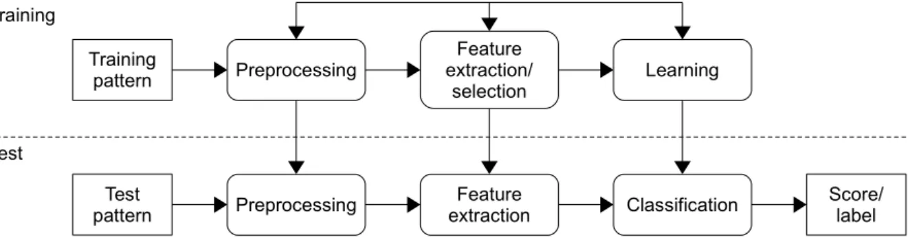
radiolo-1.2 Pattern recognition as the foundation of CAD 3 Training Test Preprocessing Test pattern Training pattern Preprocessing Feature extraction Feature extraction/ selection Classification Learning Score/ label Figure 1.1. General scheme for supervised classification. Adapted from Jain et al.18

gist can reconsider those areas prompted by the system.5 Although several studies have demonstrated the added value of CAD,2,9,10 alternative work has shown rather disap-pointing results.11,12 An explanation provided for the latter is that observer errors are often attributable to misinterpretation and not to oversight; consequently, the existing CAD technology is not addressing the right problem.13 _{Acknowledging this issue,}

re-searchers have lately investigated different ways of applying CAD and have proposed specific methods and protocols to improve interpretation.13,14 _{In addition, some more}

radical approaches have conceived CAD as a truly independent reader.15–17

1.2 Pattern recognition as the foundation of CAD

Pattern recognition is the study of how machines can observe the environment, learn to distinguish patterns of interest from their background and make sound and reasonable decisions about the categories of these patterns.18 _{Given this definition, it is easy to}

see why, as indicated before, a CAD system can be fully approached from a pattern recognition perspective: a CAD system has to learn to distinguish between normal and abnormal patterns in order to properly inform the user. For such learning to occur, a particular strategy, known as supervised classification, is typically followed. According to this strategy, a set of labeled examples belonging to the classes of interest is utilized to construct a decision rule that can be later applied to unlabeled data. A general scheme with the steps taken to perform supervised classification is shown in Figure 1.1. Similar steps are followed by a CAD system to fulfill its detection task.

During the preprocessing step, several operations that contribute to defining a com-pact representation of the patterns of interest are carried out. Common preprocessing procedures include noise removal, pattern normalization and pattern segmentation. In a CAD system, preprocessing may be applied to enhance the input images or to reduce the differences among them, which is frequently a significant issue resulting from dif-ferent acquisition devices or settings being used. Although humans seem to be quite capable of ignoring variations that are not relevant to detection, CAD algorithms should

(11)

4 Introduction

be explicitly prepared to deal with them. Another important preprocessing procedure is segmenting the region of interest from the input image. Since most detection problems concern specific anatomical structures (e.g., lungs, prostate, breasts), these structures are usually isolated so all the subsequent processing is restricted to the pertinent regions. This avoids both unnecessary computation and focusing on irrelevant patterns.

In the feature extraction step, features to represent the input patterns in such a way that the different classes can be discriminated are found. In the case of CAD, fea-tures are derived from image characteristics and are often based on knowledge about the performed task. For instance, it is known that spiculation in a mass is suggestive of malignancy.19 _{Accordingly, several CAD systems for cancer detection attempt to}

char-acterize image regions in terms of this feature.20–22 _{As not all the specific knowledge can}

be encoded into computational algorithms, general object properties, such as shape or texture, may also be taken into account. Given the amount of research conducted in the computer vision field, a large number of potentially suitable descriptors are readily available. However, since not every plausible feature is necessarily useful, and some fea-tures may even be detrimental, determining which ones are the most advantageous is an important matter to bring into consideration. Moreover, the curse of dimensionality, a well-known problem in which the required number of training points is an exponential function of the number of features, is a strong motivation for dimensionality reduction. Therefore, feature extraction is usually complemented with feature selection.

In the third step, learning and classification are carried out. In training mode, a classifier learns to appropriately partition the feature space from a set of data labeled according to the defined classes. In testing mode, the trained classifier assigns unlabeled input patterns to one of these classes. A typical classification example in CAD is to predict if the examined tissue is diseased or healthy. As with this example, common CAD applications involve binary classification problems (two classes). Additionally, supervised classification can be used to segment anatomical structures as part of the preprocessing step described before. The goal, in that case, is to decide if the analyzed regions belong or not to the sought structure. Although, in strict terms, classification implies that a single class label per pattern is assigned, most classifiers are able to output a set of scores relating each pattern with all the available classes. Depending on the objective of the task at hand, either alternative, respectively referred to as hard and soft classification, may be preferred.

Once the output of the classification component is obtained, the performance of the complete pattern recognizer can be evaluated. In CAD applications, this is fre-quently done by means of receiver operating characteristic (ROC)23 _{and free-response}

ROC (FROC)24 analysis. The empirical ROC curve is constructed by plotting pairs of observed rates, sensitivity versus specificity, resulting from applying different thresholds

(12)

1.3 Breast cancer screening 5

to the classifier’s score. Here, sensitivity is computed as the fraction of positive objects (i.e., those having a condition) being correctly labeled as positive, and specificity is com-puted as the fraction of negative objects (i.e., those not having a condition) correctly labeled as negative. A usual measure derived from the ROC curve is the area under the curve (AUC), which estimates the probability of correctly ranking a random pair of pos-itive and negative objects according to the classifier’s score. An AUC of one indicates perfect classification, whereas an AUC of 0.5 is equivalent to random guessing. The FROC curve is analogous to the ROC curve, except that it enables the analysis of cases where the condition is multifocal (i.e., there could be one or more diseased regions, and a location is associated with each of them). Since, contrary to the ROC curve, the FROC curve does not have an upper bound on the negative object axis, the partial AUC is used instead of the AUC. Besides sensitivity and specificity, and the summarizing measures derived from the ROC and FROC curves, indicators such as the positive predictive value (PPV), defined as the percentage of objects labeled as positive that are truly positive, and the negative predictive value (NPV), defined as the percentage of objects labeled as negative that are truly negative, are utilized, particularly in screening. A relevant aspect of both PPV and NPV is that they take into account prevalence, which is the proportion of a population found to have a condition.

A final detail to notice regarding the classification scheme provided in Figure 1.1 are the feedback links among the training blocks. They allow the designer to optimize the strategies taken at each step depending on the previously or subsequently obtained outcomes. In the context of an interdisciplinary technology such as CAD, this refine-ment mechanism is of especial importance, as it is the main means of ensuring proper interaction among the different combined elements.

1.3 Breast cancer screening

As the name suggests, breast cancer is cancer that forms in tissues of the breast. The most common types of breast cancer are ductal carcinoma, which begins in the lining of the milk ducts, and lobular carcinoma, which begins in the lobules (milk glands) of the breast. Of the known cancers, breast cancer is the most frequent and the leading cause of cancer deaths among women worldwide. According to the latest statistics,25 almost 1.7 million women were diagnosed with breast cancer and more than half a million died of this disease in 2012. Although several risk factors, such as familial history or reproductive issues, have been well documented,26 _{the specific cause of breast cancer}

in the majority of cases cannot yet be identified. As a result, effective mechanisms of prevention are difficult, which renders early detection the best available option.

(13)

6 Introduction

morbidity and mortality by increasing the chances of full recovery due to a more effective treatment. To take advantage of this potential, several countries have implemented breast cancer screening programs in which asymptomatic women in a determined age group are periodically invited for examination. In the Netherlands, for example, the national program is directed at women between 50 and 75 years, and establishes a two-year period between screening rounds. While several studies have shown the effectiveness of screening along its history,27–30 some recent publications31–33 have raised controversy by stating that only a limited benefit in terms of breast cancer death prevention has been observed. One of the main arguments given to refute this negative conclusion is that the real effect of screening can only be appreciated in the long term.34–36

The most common test performed for breast cancer screening is mammography, which uses low-dose X-rays to examine the breasts. During the procedure, the breast is compressed using parallel plates so the tissue thickness is evened out and the target is kept fixed. This contributes to improving the detection of small abnormalities by increasing the image quality and minimizing the motion blur. In ordinary screening, up to four images are acquired. They correspond to the mediolateral oblique (MLO) and the craniocaudal (CC) projections for both the left and the right breasts. Com-bined information from the MLO and CC views is used to check if a space occupying lesion is visible on both images, in which case, the likelihood of malignancy is higher. Combined information from the left and the right breasts is used to detect asymmetry, which is also believed to be a malignancy indicator. Further, by comparing the current mammograms with the ones obtained in previous screening rounds, suspicious tissue changes can be identified.

Mammographic manifestations of cancer can be roughly divided into microcalcifica-tions and masses. Microcalcificamicrocalcifica-tions are calcium deposits that appear as small, high-intensity specks on a mammogram. They can be distributed in one or more clusters, fill a segment of the breast or be scattered over the entire breast. Usually, microcalcifications are associated with noncancerous extra cell growth; however, clusters of microcalcifi-cations can sometimes occur in areas of early cancer. Thus, depending on how they are clustered, and their shape, size and number microcalcifications may raise concern. An example of a malignant cluster of microcalcifications is shown in Figure 1.2 (left). Masses are space occupying lesions with a circumscribed, indistinct or spiculated margin. Spiculation, in particular, is considered an important sign of malignancy.19 _{As shown in}

Figure 1.2 (right), spiculation is a stellate pattern of line-like structures directed from the margin to the center of a mass. Irregular mass margins may also be attributed to cancer, whereas sharp, circumscribed borders are often an indication of a benign process. In practice, besides the previous definition, the term “masses” may include lesions such as architectural distortions and asymmetric densities.

(14)

1.4 Tuberculosis detection 7

Figure 1.2. Mammographic manifestations of cancer: a cluster of microcalcifications (left) and a spiculated mass (right).

Interpretation of mammography is a difficult task; therefore, it has become an at-tractive target for CAD application since the early developments.8 In fact, one of the first CAD systems approved for clinical use aimed at detecting breast cancer on digitized mammograms.37 _{Nowadays, several similar systems are commercially available, and in}

the United States, the majority of the screening mammograms are read with CAD.38

Notwithstanding, despite years of research, both in industry and academy, the effec-tiveness of CAD for screening mammography is still questioned. More precisely, while the detection performance of current CAD systems on microcalcifications is relatively high and well recognized by radiologists, there is less agreement on the benefit for mass detection.39 _{Being the latter a more challenging problem, development of radically new}

or an update to previously established algorithms seem key to further achievements. Chapter 2 presents a contribution in this line. Additionally, disappointing results of CAD may be due to the way it is currently applied. Recall that the adopted protocol restricts CAD systems to be mere prompting tools. In this respect, different ways of exploiting CAD should be explored. Notable approaches such as “interactive CAD”13

and “CAD for independent reading”15 _{have already been proposed. In Chapter 3, yet}

another alternative, “postscreening CAD,” is investigated.

1.4 Tuberculosis detection

Tuberculosis (TB) is an infectious disease caused by Mycobacterium tuberculosis and other TB complex members. It can affect practically any human organ but is most fre-quently associated with the lungs, as the bacilli grow better in tissues with high oxygen content.40 _{In lung infection, M. tuberculosis is typically inhaled and passed through the}

airways to the alveolar space, where it mainly targets macrophages and other mononu-clear phagocytes.41 Progression of the infection may promote the formation of

(15)

granu-8 Introduction

lomas, destruction of lung tissue and further dissemination through the bloodstream. Although, in most cases, the organism’s adaptive immune response is enough to contain that progression (which leads to an asymptomatic state known as latent TB infection), when immune deficiencies are present (e.g., due to HIV infection), failure to control the bacteria results in active disease.

Common symptoms of active TB are, for instance, fever, weight loss, night sweats and chronic cough. Further, since the bacilli are present in the sputum, subjects with active TB are able to infect others by coughing or sneezing. This simple transmission mechanism is probably one of the main factors that have made TB a worldwide health problem. It is estimated that one-third of the world’s population has latent TB infection. From this population, around nine million people develop active disease every year, with most of the burden corresponding to middle- and low-income countries, especially in Asia and Africa.42 _{The mortality rates associated with TB are high as well.} _In

fact, despite affordable and effective treatment being available, TB remains one of the world’s deadliest communicable diseases, accounting for 1.5 million deaths per year.42

In this regard, accurate and rapid diagnosis is of paramount importance to ensure that individuals with active disease are properly treated.

Definitive diagnosis of TB is often performed through sputum culture, which is con-sidered the gold standard. However, although this test yields the highest sensitivity, it also takes the longest time to produce its results, which may vary from two to four weeks and is a direct consequence of the slow growing rate of M. tuberculosis.40

More-over, implementing the method is relatively expensive and requires good laboratory facilities; therefore, it is difficult to deploy in resource-constrained settings. This issue has led smear microscopy, a 100-year-old test, to become the main diagnosis option in low-income countries. Smear microscopy is relatively easy to perform and has high specificity but suffers from low sensitivity, notably in patients with advanced HIV dis-ease.40 In recent years, the advent of nucleic acid amplification techniques has been the most promising development in TB diagnosis. One test, in particular, known as Xpert MTB/RIF assay, has shown both high sensitivity and specificity, and has been endorsed by the World Health Organization in 2010. An additional advantage of Xpert MTB/RIF is that results can be obtained in only two hours. Unfortunately, the cost of the test is relatively high, which poses a serious problem for its massive utilization in restricted settings. To circumvent this problem, screening strategies involving symptom evaluation and, more prominently, chest radiography have been proposed.43,44 _Inspired

by these strategies, an automated screening alternative combining the same cues has been developed as part of this thesis (Chapter 6).

The renewed interest in chest radiography in the context of TB diagnosis algorithms has been largely motivated by the introduction of digital devices, which among others,

(16)

1.4 Tuberculosis detection 9

Figure 1.3. Radiographic manifestations of TB. From left to right: small opacities (affecting most of the lung), large opacities (top part of the lung) and consolidation (bottom part of the lung).

has decreased the cost and the effort required for the test by eliminating the need for film and chemicals, and the whole developing process. Moreover, the quality of the images has been considerably improved. Digital radiography has also accelerated the development of CAD by simplifying the collection of image data. In its current stage, CAD may be able to address one of the main disadvantages of radiological tests, which is the need for qualified experts to assess the images. The lack of this kind of personnel has been a major barrier to chest radiography usage in low-resource countries. Another historical problem of chest radiography has been the interpretation process itself, as disagreement between readers has been frequently observed.45–47 _{CAD may also offer a}

solution to this problem by providing objective and consistent results.

The standard chest radiograph (CXR) view utilized for TB examination corresponds to a posterior anterior (PA) acquisition, in which the patient faces the imaging plane, and the X-rays enter through the posterior side and exit through the anterior side. Typical TB manifestations sought on this PA CXR include small opacities, which are small foci surrounded by still-healthy tissue that resemble a dotted pattern; large opac-ities, which are a product of an increased inflammation and destruction of more tissue; and consolidation, which is an increase of fluid in spaces surrounding the lung.∗ Some illustrative examples are shown in Figure 1.3. As can be seen on the examples, the afore-mentioned manifestations exhibit some particular textural properties that allow their discrimination from the healthy lung parenchyma. These properties are heavily ex-ploited by most of the computerized TB detection methods reported in the literature.49 In Chapters 4 and 5, a CAD system targeting this kind of textural abnormalities is used as a basis for experimentation.

(17)

10 Introduction

1.5 Thesis outline

As indicated before, the aim of this thesis is to expand the capabilities of CAD systems by means of effective pattern recognition. This has been accomplished both by pushing the limits of already established techniques, as well as by addressing their limitations. Considering the general scheme given in Section 1.2, two core components: feature ex-traction and selection, and learning and classification have been the main focus. The tackled issues and the developed methods are presented in the chapters of this thesis as outlined bellow.

Chapter 2 deals with the problem of feature discrepancy in image location classi-fication. In mammography-based cancer detection and other CAD applications, the observed lesions are focal and have a distinct location. For that reason, specific feature extractors yielding a peaked response in the presence of these lesions are often utilized. However, due to pattern variability and other factors, the responses of different features may not be well matched. This may prevent their optimal combination during learning and classification. As a solution, strategies applying feature maxima propagation and local feature selection are proposed.

Chapter 3 investigates CAD operation at very high specificity. The objective is to develop a standalone postscreening system for detecting early signs of malignant masses that could be missed by screening radiologists. In such a scenario, a highly specific system is necessary to avoid a significant impact on the recall rate. These operating conditions are radically different from traditional CAD settings that prioritize sensitivity in order to minimize oversight errors. The crucial aspect of the investigated system is to optimize its learning component in such a way that it reaches reasonable sensitivity while preserving high specificity. For that purpose, a large number of normal cases, approximating the data distribution found in screening, is taken into account.

Chapter 4 centers on the issues arising in data labeling for training and optimiza-tion. Detailed labeling, as required by the supervised scheme described in Section 1.2, demands a considerable amount of effort. It may also be error prone, especially in cases where nonfocal disease patterns are to be outlined. Under adverse circumstances, de-tailedly annotated data or the expertise to obtain them may simply be unavailable. As a consequence, any supervised approach becomes inapplicable. To address these issues, multiple-instance learning (MIL), a learning paradigm that assigns labels to groups of patterns instead of individual instances, is adopted. This allows a CAD system to be trained with image labels instead of pixel labels obtained from annotated lesions. To evaluate this alternative strategy, a MIL-based CAD system designed to detect textu-ral TB manifestations is compared with its supervised counterpart through different operating conditions.

(18)

1.5 Thesis outline 11

Chapter 5 tackles the problem of uncertainty inherent to MIL. Although MIL leads to a simplified labeling approach beneficial for CAD, it also leads to uncertainty, as the labels of individual instances are not directly known. To deal with this problem, several MIL algorithms attempt to infer the unknown labels based on the known information. However, imputation of data may be difficult and uncertainty may not be removed to the desired extent. Perhaps, under those conditions, certain labeling is still the best alternative, and the key is to obtain this labeling with the minimum effort. To this end, active learning (AL) is applied, and a new training algorithm combining MIL and AL is developed. This new algorithm further refines the system introduced in the previous chapter and improves its performance in terms of lesion localization and false-positive detections.

Chapter 6 explores the use of nonimage data as a complementary input in CAD. Besides image data, there is often clinical information available in the medical context. While this information is ordinarily exploited by human experts, it is largely disregarded by CAD algorithms. Since CAD capabilities may be limited by the utilized images themselves, incorporating other types of cues could be a good alternative to improve performance. To capitalize on this point, a combination framework based on state-of-the-art feature ranking and selection, and multiple learner fusion is proposed. A pstate-of-the-articular configuration combining CXR CAD scores and TB-related indicators is applied to the task of TB detection.

(19)

(20)

Mass candidate detection

2

J. Melendez, C. I. S´anchez, B. van Ginneken, N. Karssemeijer

Original title: Improving mass candidate detection in mammograms via feature maxima propagation and local feature selection

(21)

14 Mass candidate detection

Abstract

Mass candidate detection is a crucial component of multistep computer-aided detection (CAD) systems dealing with breast cancer. It is usually performed by combining several local features by means of a classifier. When these features are processed on a per-image-location basis (e.g., for each pixel), mismatching problems may arise while constructing feature vectors for classification, which is especially true when the behavior expected from the evaluated features is a peaked response due to the presence of a mass. In this study, two of these problems, consisting in maxima misalignment and differences of max-ima spread, are identified, and two solutions are proposed. The first solution, feature maxima propagation, reproduces feature maxima through their neighboring locations. The second solution, local feature selection, combines different subsets of features for different feature vectors associated with image locations. Both alternatives can be ap-plied independently or together. They are included in a mammogram-based CAD system intended for mass detection in screening. Experiments are carried out with a database of 382 digital cases. Sensitivity is assessed at two sets of operating points. The first one is the interval from 3.5 to 15 false positives per image (FPs/image), which is typical for mass candidate detection. The second one is 1 FP/image, which allows estimating the quality of the mass candidate detector’s output for use in subsequent steps of the CAD system. The best results are obtained when the proposed methods are applied together. In that case, the mean sensitivity in the interval from 3.5 to 15 FPs/image significantly increases from 0.926 to 0.958 (p <0.0002). At the lower rate of 1 FP/image, the mean sensitivity increases from 0.628 to 0.734 (p < 0.0002). Given the improved detection performance, it is believed that the strategies proposed in this study can render mass candidate detection approaches based on image location classification more robust to feature discrepancies and prove advantageous not only at the candidate detection level but also at subsequent steps of a CAD system.

(22)

2.1 Introduction 15

2.1 Introduction

It is well known that assessment of screening mammography is a complex task. Thus, to assist radiologists during breast cancer screening, computer-aided detection (CAD) systems are being developed. In the majority of cases, the sought abnormalities are either microcalcifications or masses, being the latter the most difficult to detect due to their large variation in size and shape, and their poor image contrast. Therefore, considerable effort is devoted to improving CAD systems for detecting malignant masses as in the case of the current study.

CAD systems dealing with mass detection usually comprise multiple steps.50–52_{In the}

initial step, a set of mass candidate locations is determined based on local image features. These features are typically processed by a classifier, which assigns a mass likelihood score to each image location. Then, those locations associated with a high score are identified as mass candidates and segmented. By adjusting the threshold applied to the classifier’s output, the sensitivity of the initial step can be varied. It is common to set this sensitivity to a relatively high value in such a way that most potential abnormalities are detected. However, due to misinterpretation of normal structures, the number of false-positive detections is relatively high as well. Therefore, in the following steps, the candidate regions are further processed, usually by considering a more elaborate set of features. Since the performance of the subsequent steps strongly depends on the quality of the candidate regions, the initial detection step is a key component of the complete system. Furthermore, the masses missed during this step cannot be recovered later. Ideally, the initial detection step should reach its maximum sensitivity with the minimum number of false positives. In this way, the subsequent steps could focus on a more specific problem and achieve better solutions, as they would not be influenced by irrelevant patterns that could be filtered during the initial step.

Features used for mass detection can be related to gray-level intensities, local texture or morphological measures.53In addition, it is common to take the distribution of spicules associated with masses into account. Spiculation is an effective indicator of malignancy in masses, as more than half of the screening-detected cancerous masses show this pattern.19

However, the remaining lesions may only be detectable by the mass itself. Thus, in order to deal with the different cases, it is also common to extract gradient orientation information. The orientation of gradient vectors can provide an idea of the location of a mass’ center. Since the shape of a mass is approximately rounded, an image pixel located close to the center is expected to have most of its surrounding gradient vectors pointing to itself. As can be seen from the above, both spiculation and gradient orientation features seem to naturally complement each other. Therefore, including those features in a CAD system can be an important strategy for breast cancer detection.

(23)

Several approaches reported in the literature have implemented spiculation and gra-dient features for mass detection. For instance, Kobatake et al.54 _{applied the Iris filter,}

which measures the convergence of gradient vectors at a given pixel, to enhance rounded opacities. Later, they extracted morphological line-skeletons for spicule enhancement.55

Karssemeijer and te Brake20,56 _{developed a method based on analysis of local gradient}

concentration and line orientation after filtering the input image with a set of first- and second-order directional Gaussian derivatives. In related work,57 Karssemeijer intro-duced an efficient approach that computed features as a continuous function of spatial scale. Zwiggelaar et al.21 modeled the center of a mass and the surrounding pattern of linear structures using a directional recursive median filter and a multiscale directional line detector, respectively. Liu et al.22 _{detected spiculated lesions by means of a}

top-down multiresolution scheme based on linear phase nonseparable wavelets. Sampat and Bovik58 _{applied the Radom transform for spicule enhancement and then determined the}

convergence location with a set of radial spiculation filters. Wei et al.50 _{computed the}

average gradient direction over neighboring concentric annular regions around a pixel to identify regions of interest. Sakellaropoulos et al.59 _{extracted intensity and gradient}

orientation features after wavelet decomposition to detect masses in dense parenchyma. Mencattini and Salmeri60 evaluated the eigenvalues of the Hessian matrix obtained from the gradient image and proceeded to locate “wells,” which according to the authors can be associated with masses. Other related approaches can be found in the review by Oliver et al.53

Most of the aforementioned features are designed to attain their maximum response at the center of a mass. Therefore, the task of labeling image locations as normal or abnormal corresponds to segregating the peaks resulting in the feature domain. This is not a simple task. Thus, in order to achieve the best performance, the common approach is to combine several features by means of elaborate classification techniques. However, due to the large variability of the processed images, the theoretical properties expected from these features are not always observed, and problems during classifica-tion may arise. We have identified two of these problems:

1. The maxima among several features that characterize a given mass may not oc-cur at the same image location. Since feature vectors for classification are con-structed on a per-image-location basis at this point, these maxima may never be part of the same feature vector, which is undesirable, as it dims the discrimina-tion power of the combined features.

2. Although the ideal output of these features is a well-defined peak at the center of a mass, in practice, lesions may be far from the ideal model for which a particular feature was designed and may show distorted or scattered patterns,

(24)

2.1 Introduction 17

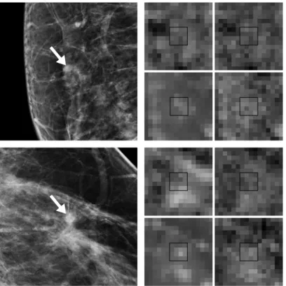
Figure 2.1. A mammographic image with a malignant mass (left) and two of its associated feature images obtained by means of the spiculation-based (middle) and gradient orientation-based (right) feature extractors developed by Karssemeijer and te Brake.20,56,57 _{Features were computed according}

to an eight by eight pixel grid. Lighter gray levels indicate higher feature values. The region where the mass is located is shown magnified in order to better appreciate the differences in peak location and spread yielded by the two features.

or appear at a different scale. Consequently, the resulting output may not be clearly concentrated at a specific location but span several neighboring locations instead. If several features are combined, differences in peak spread are likely to occur. Depending on how large these differences are and the proportion of discrepant data, the coherence of the feature vectors may be compromised, and the classifier may not be able to optimally determine appropriate relations among the features.

Figure 2.1 illustrates an example of both discussed problems. In this figure, a mam-mographic image with a malignant mass (left) and two of its associated feature images (middle and right) are shown. From the magnified crops of the feature images, a dis-placement of two locations can be observed between the maxima of the peaks charac-terizing the lesion. Moreover, the peak corresponding to the first feature (middle) is substantially wider than the one corresponding to the second feature (right). Thus, even if they were aligned (with respect to their maxima), a mismatch would still exist in the following sense: while the location corresponding to the maximum in the narrow peak would be paired with the maximum of the wide peak, the neighboring locations around the center of the narrow peak, which have much lower values, would still be paired with high values in the wide peak. As a result, it would be difficult to establish a coherent pattern made up of high responses for masses.

(25)

operates at the feature level and propagates (and hence aligns) the feature maxima through a given neighborhood. The second strategy operates at the classifier level and relies on the observation that the issues mentioned before do not always occur in all the available features; therefore, exploiting the interaction of particular subsets of features for particular subsets of samples seems an appropriate choice. This is accomplished by means of a random forest classifier.61 In addition, we investigate the effect of combining both strategies. We demonstrate the effectiveness of the proposed approaches via a CAD application consisting in mass candidate detection in screening mammography. The features used by the CAD system are based on the gradient orientation and spiculation measures derived by Karssemeijer and te Brake.20,56,57

2.2 Materials

The Dutch screening program targets women between 50 and 75 years, and invites them to participate in a free, nationwide breast cancer screening service every two years. Further information can be found elsewhere.62 _{The cases utilized in this study were}

acquired in the course of this program in the period 2003–2008 at both the Foundation of Population Screening Mid-West in Utrecht and the Radboud University Medical Center in Nijmegen. In accordance with the Dutch guidelines, the mediolateral oblique (MLO) and craniocaudal (CC) views were obtained only at the initial screening, whereas at subsequent rounds, only the MLO view was obtained, unless an indication that acquiring the second view was beneficial existed.

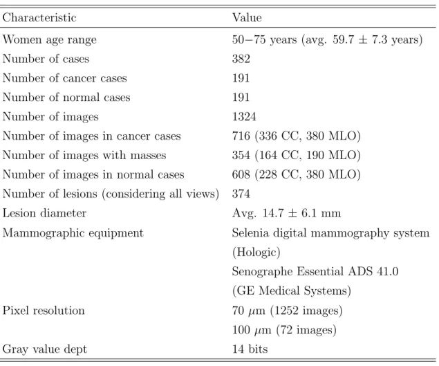
Mammograms with abnormalities were annotated under the supervision of an ex-perienced radiologist. These annotations were used as the reference standard during evaluation. For our experiments, a set of 328 digital cases sampled from a cohort of more than 50 000 cases available in our databases was selected. The set consisted of 191 cases with a biopsy-proven malignant mass and 191 cases without cancer. Both cases with MLO, or CC and MLO views were included. Cases in which lesions other than masses (e.g., microcalcifications, architectural distortions, etc.) were the only sign of malignancy were excluded. Cases with only benign lesions were excluded as well. This yielded a total of 169 cases that were included in the abnormal subset. To make the problem more challenging, we also searched for digital screening mammograms ac-quired prior to detection in which masses were already visible. This accounted for 22 more cases, which completed the total of 191 cancers mentioned above. The remaining 191 noncancer cases were digital mammograms that were not referred during screening and had at least one normal follow-up exam. These mammograms were randomly se-lected among the noncancer cases available in our databases. Further details about our experimental data set are given in Table 2.1.

(26)

2.3 Methods 19

Table 2.1. Characteristics of the mammogram data set utilized in this study

Characteristic Value

Women age range 50−75 years (avg. 59.7 ± 7.3 years)

Number of cases 382

Number of cancer cases 191

Number of normal cases 191

Number of images 1324

Number of images in cancer cases 716 (336 CC, 380 MLO)

Number of images with masses 354 (164 CC, 190 MLO)

Number of images in normal cases 608 (228 CC, 380 MLO) Number of lesions (considering all views) 374

Lesion diameter Avg. 14.7 ±6.1 mm

Mammographic equipment Selenia digital mammography system

(Hologic)

Senographe Essential ADS 41.0 (GE Medical Systems)

Pixel resolution 70µm (1252 images)

100 µm (72 images)

Gray value dept 14 bits

2.3 Methods

2.3.1 Mass candidate detection in mammography-based CAD

The CAD system utilized in this study closely follows the multistep paradigm described before. Considering its single-view mode, two main steps can be identified. In the first step, a set of basic features20,56,57 is computed, and a classifier is utilized to determine a set of candidate regions. In the second step, these regions are further processed by computing a richer set of features, and a new classification process is carried out to get the final malignancy score. More details can be found in related work.52 _{Since we}

are interested in the mass candidate detection problem, we focus on the first step of this system. This baseline mass candidate detector (or baseline detector in short) in turn consists of three steps: image preprocessing, feature extraction and image location classification. Figure 2.2 shows a flowchart of this baseline detector with its three steps, as well as the improvements proposed in this study (Sections 2.3.2 and 2.3.3). A description of each step is given next.

(27)

20 Mass candidate detection Image preprocessing Input image Feature extraction Image location classification Mass candidates Baseline mass candidate detector

Feature maxima

propagation Local featureselection

Proposed improvements

Figure 2.2. Flowchart of the baseline mass candidate detector showing its three steps: image pre-processing, feature extraction and image location classification, and the improvements proposed in this study, namely feature maxima propagation (Section 2.3.2) and local feature selection (Section 2.3.3).

Image preprocessing

Prior to mass detection, raw input images are preprocessed. In the first step, a given image is downsampled to a resolution of 200 µm per pixel by means of bilinear inter-polation. Then, the image is segmented into breast area, pectoral muscle (if it is an MLO view) and background. Background pixels are identified by applying thresholding and a sequence of morphological operators.63 Subsequently, the pectoral muscle is seg-mented from the breast area by fitting a straight line to its boundary using a modified Hough transform.63 Since this boundary is typically slightly curved, an optimal path search considering the previous initial estimate is performed afterwards. In the next step, the raw image is converted to a standard representation by simulating the film-based mammogram acquisition procedure.64 _{However, instead of modeling the relation}

between intensity values and exposure with a nonlinear characteristic curve, a piece-wise linear model is utilized. This approach follows more closely the linear relation between (logarithmic) exposure and tissue thickness established by Engeland et al.;65_{therefore, it}

provides a better image representation. The model parameters were determined in a set of independent experiments. After image conversion, a thickness equalization algorithm is applied to enhance the periphery of the breast.66 A similar algorithm is used on MLO images to equalize the intensity of the pectoral muscle in order to facilitate detection of masses located on or near the pectoral boundary.

Feature extraction

As stated before, in this study we utilized the spiculation- and gradient-based feature extractors developed by Karssemeijer and te Brake.20,56,57 _{Spiculation characterization}

involves detecting line-like patterns radiating from a central location. Line orientation estimates for the image pixels are obtained from the output of directional second-order

(28)

2.3 Methods 21

Gaussian derivative operators. The orientation at which these operators have the maxi-mum response is selected. The distribution of these estimates is analyzed for each image location considering a circular neighborhood. By imposing a selection criterion on the intensity of the filter output, a subset of pixels within this neighborhood, representing potential sites of interest, is determined. To calculate the features, all the pixels from this subset that are directed towards the center of the neighborhood are counted as a function of the direction in which they are located. Discrete directions are obtained by dividing the neighboring space into a number of radial bins. To achieve a multiscale representation, cumulative normalized counting is performed as a function of the radius. The first feature derived from this analysis, denoted as l1, is related to the maximum

number of pixels whose direction points to the center of the neighborhood and gives a measure of the maximum spiculation. The radius at which this maximum occurs, de-noted aslr, is used as a second feature. Since pixels oriented towards a location can be

found only in a few directions, and thus it is not very likely that the site being evaluated belongs to the center of a spiculated lesion, a third feature, denoted asl2, measuring in

how many directions spiculation is strong is defined. A similar procedure and reasoning is followed to compute the gradient-based features. In this case, however, first-order derivatives are utilized and only two features, denoted as g1 and g2, are defined. They

are analogous tol1 and l2. The five features described so far are extracted for locations

inside the tissue area sampled at 1.6 mm (every 8 pixels). This setting is a compromise aiming at decreasing the computational load while preserving the capability of detecting small masses.56 _{The resulting feature images are smoothed with a Gaussian kernel with}

σ= 1.6 mm before classification.

Image location classification

Location classification is carried out by an ensemble of five neural networks. Each of these networks is a multilayer perceptron with randomly initialized weights and utilizes a different ratio, ρ, ρ = 0.1, . . . ,0.5, of positive to negative training patterns. The remaining settings are shared among the networks and are configured as follows: there are five input neurons, five neurons in the single hidden layer and one neuron in the output layer; all neurons are configured with a sigmoid function. The standard backpropagation algorithm is used to train the networks to map abnormal patterns to a value close to one and normal patterns to a value close to zero. Training is carried out until 106 _patterns

are processed. The learning rate is set to 0.005. During classification, averaging of the networks’ outputs results in an image whose pixel values represent the likelihood of a mass being present. This likelihood map is then slightly smoothed and its local maxima are determined. A local maximum is selected as a candidate location when its likelihood

(29)

is above a certain threshold. This yields a list of locations that are of interest for further investigation. Before training and classification, features are scaled to have zero mean and unit standard deviation using the training set.

2.3.2 Feature maxima propagation

As discussed before, misalignment and differences of spread among feature maxima may pose serious problems when performing image location classification. In order to alleviate these problems, we propose to propagate the maxima of relevant features through a given neighborhood. This is accomplished by means of themaximum filtering algorithm described below:

1. For each feature image location F(i, j) that belongs to the tissue area, define a circular neighborhood N with radius R centered at location F(i, j). Members of this neighborhood are only those locations that belong to the tissue area as well. 2. Determine the maximum value of the neighborhood.

3. Assign this value to F0(i, j), which is the location corresponding to F(i, j) on a temporary feature image.

4. Once all valid image locations have been explored, replace their original values

F(i, j) with the temporary values F0(i, j).

Considering our particular application, the proposed algorithm is intended to be applied at the end of the feature extraction step described in Section 2.3.1, prior to Gaussian smoothing (see also Figure 2.2). It is worth to mention that, although all the features with relevant peaks could be processed, such an approach is not necessary. In a pilot experiment, we verified that applying the maximum filter only to the gradient-based features (g1 andg2), so their maxima were aligned and propagated with respect to

their spiculation-based counterparts (l1 and l2), yielded comparable results as filtering

all of them. Therefore, this approach was followed in the current study.

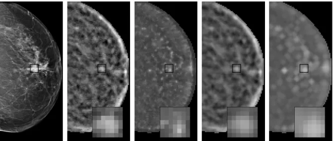
Figure 2.3 shows the feature images corresponding to Figure 2.1 once maximum fil-tering (and Gaussian smoothing) have been carried out. In this case, g1 (far right) was

processed with a maximum filter configured withR = 3.2 mm, whilel1 (right) remained

unprocessed. Comparing both feature images, it is possible to observe that the peak alignment is not perfect in the sense that the gap between the maxima still exists. How-ever, the neighbors of the maxima, which now have very close values, are indeed aligned. In addition, the width of the peak ing1better matches the width of the peak inl1, which

leads to a better overlap and thus increases the chances of having correct representative values of both peaks in the same feature vectors. Although it can be argued that with

(30)

2.3 Methods 23

Figure 2.3. The effect of applying the proposed maximum filtering algorithm to the gradient-based feature image shown in Figure 2.1 (right). From left to right: original mammographic image, original spiculation-based feature image, original gradient-based feature image, smoothed spiculation-based fea-ture image and smoothed gradient-based feafea-ture image after maximum filtering. Note that although the maxima in the last two feature images are still misaligned, locations with very close values are now matched.

a larger radius a better match in alignment and overlap could be obtained, such a set-ting could also increase the distortion in the feature image and lead to “enhancement” of irrelevant locations that do not belong to a lesion pattern. Ideally, a compromise be-tween enhancement and distortion should be determined. Consequently, in this study we also investigated the effect of different neighborhood radii on detection performance (Section 2.3.4).

2.3.3 Local feature selection

Since maxima misalignment and differences in maxima spread do not always occur si-multaneously in all the features, considering only the interactions of those features that do not show the aforementioned issues may lead to improved classification performance. Unfortunately, there is no way to know a priori which subsets of features are the most suitable for each particular case, as this condition may be different for a large number of image locations and their associated feature vectors. This makes the application of any feature selection method that estimates the relevance of features globally and only once per data set inappropriate. Therefore, in this study we investigate a particular classification technique, random forests,61 _{which incorporates a local feature selection}

mechanism as part of its learning and classification algorithms, and thus realizes (to a certain extent) the desired strategy that processes different subsets of features for differ-ent subsets of feature vectors. This classifier constitutes an alternative to the ensemble

(31)

of neural networks described in Section 2.3.1 (see Figure 2.2 as well).

A random forest is an ensemble of tree predictors that can deal with both classification and regression problems. For classification, the algorithm takes the input feature vector, classifies it with every tree in the forest and outputs the class label that receives the majority of votes. For regression, the output is the average of the outputs over all trees. We used regression trees in order to obtain a continuous output. The following algorithm was utilized to construct each regression tree in the ensemble:

1. Let the number of cases in the training set be N. Sample N cases at random with replacement from the original data and use these cases as a training set for the tree.

2. Let the number of features in the data set beM. Define a numberm,m < M, such that at each tree node, m features are randomly selected in order to determine the best split.

3. Grow the tree to the largest possible extent and do not prune it.

By carefully analyzing the previous algorithm, it is possible to identify a number of reasons why the random forest framework would be capable of achieving the desired local feature selection effect. First, themrandomly selected features are utilized at each tree node to determine the best split. Since the training set is continuously partitioned through the nodes of the tree, different subsets of feature vectors comprising different subsets of features are explored. This increases the chances that correctly constructed feature vectors are evaluated. Second, since there are usually several nodes (due to the lack of pruning) and several (independent) trees in a given forest, a wide variety of combinations are explored by the whole ensemble. By adding this to the previous point, diversity is further increased. Thus, we expect that the appropriate feature interactions can be learned with the appropriate feature vectors. Finally, in the same line as above, having different training sets for every tree in the ensemble also contributes (although to a lesser extent) to diversification.

Breiman61 _{showed that the generalization error of a random forest depends on the}

interplay between two parameters: the strength of each individual classifier and the correlation between any two individual classifiers. He also showed that increasing the strength of the trees decreases the forest error, while increasing the correlation increases this error. Moreover, reducing or increasingmrespectively reduces or increases both the strength and correlation, which means that an optimal range ofm could be determined. This seems to be the only adjustable parameter to which random forests are somewhat sensitive. However, Breiman also pointed out that this optimal range is usually wide. Therefore, taking into account that the number of available features in our application

(32)

2.3 Methods 25

is already low, a fixed, nonoptimized value of m was considered to suffice. Following Breiman’s approach, this value was set to the first integer lower than or equal to √M.

2.3.4 Evaluation

Detection performance was evaluated using free-response receiver operating character-istic (FROC) analysis after five-fold cross-validation. During data splitting into folds, we took care that the images corresponding to the same case were always assigned to the same fold. Moreover, the ratio of abnormal to normal cases was roughly the same in each fold. Once the five folds were processed, the likelihood scores assigned to the resulting maxima in the five test sets were pooled, and lesion-based FROC was com-puted. Sensitivity was defined as the number of detected lesions divided by the total number of lesions. A lesion was considered detected when the local maximum reported by the system was inside the reference annotated region. If several local maxima were associated with a given lesion, only the one with the highest score was counted.

To obtain a single performance measure, the mean sensitivity in a range of false positive rates on a logarithmic scale52 _{was computed as}

S(3.5,15) = 1 ln 15−ln 3.5 Z 15 3.5 s(f) f df, (2.1)

wheref is the number of false positives per normal-case image (FPs/image) and s(f) is the lesion sensitivity. Note that, in a screening setting, only the normal cases are relevant when assessing the false-positive detections. The computed measure is proportional to the partial area under the FROC curve plotted on a logarithmic scale. Using a logarithmic scale avoids that the measure is dominated by operating points at high false positive rates. The range from 3.5 to 15 FPs/image was selected based on the operating points reported in the literature for similar mass candidate detection systems.50,64,67–69

Statistical significance of the performance difference between pairs of evaluated ap-proaches was determined by means of bootstrapping.70_{Cases were sampled with}

replace-ment from the pooled cross-validation set 5000 times. Every bootstrap sample had the same number of cases as the original data set. For each new sample, two FROC curves were constructed using the likelihood scores yielded by the two methods being com-pared. Then, the difference in mean sensitivity, ∆S, was computed. After resampling 5000 times, 5000 values of ∆S were obtained. Thep-values were defined as the fraction of ∆S values that were negative or zero. Since we performed three comparisons per experiment, we applied the Bonferroni correction to the significance level. As a result, performance differences were considered significant if p <0.0167 (0.05/3).

(33)

Table 2.2. Approaches compared per experiment and their settings

Approach Neighborhood Classifier

Experiment 1

Baseline features – Neural networks (5 networks)

Maximum filtering R= 1.6 mm Neural networks (5 networks)

Experiment 2

Neural networks – Neural networks (5 networks)

Gentle adaboost – Gentle adaboost (100 stumps)

Random forest – Random forest (100 trees)

Experiment 3

Neural networks + baseline features – Neural networks (5 networks) Neural networks + max. filtering R= 1.6 mm Neural networks (5 networks)

Random forest + baseline features – Random forest (100 trees)

Random forest + max. filtering R= 1.6 mm Random forest (100 trees)

approaches. Table 2.2 summarizes the system configurations utilized in each of them. More details are given below.

In the first experiment, we compared the detection performance of the spiculation-and gradient-based features with spiculation-and without the maximum filtering algorithm described in Section 2.3.2. We also assessed the effect of using different neighborhood radii with the maximum filter. The explored values of R were 1.6, 3.2 and 6.4 mm. Classification was carried out by the ensemble of neural networks and the methodology described in Section 2.3.1.

In the second experiment, we compared the detection performance of the random forest classifier described in Section 2.3.3 with that of the ensemble of neural networks used by the baseline detector. To gain further insights from this experiment, a gentle adaboost classifier71 _{with regression stumps as weak learners was also included. We}

se-lected to compare with this technique for several reasons. First, it constitutes a classifier ensemble similar to the random forest investigated in this study. Second, it is considered a state-of-the-art classifier. Third, and most important, it results in a sort of feature selection algorithm that evaluates features according to differently weighted training sets when selecting the best classifiers for the ensemble. Consequently, it represents a point in between what we criticized in Section 2.3.3 about traditional feature selection ap-proaches and what is expected from the feature selection capabilities of random forests.

(34)

2.4 Results 27

All the compared techniques processed the same baseline features and followed the same classification methodology as described in Section 2.3.1. The number of trees utilized by the random forest was 100. This parameter value was the one that yielded the high-est mean sensitivity during parameter optimization, although by a very narrow margin, which is in accordance with the observation that, after a certain point, adding more trees to the ensemble does not significantly increase nor decrease prediction performance. We evaluated several values: 50, 100, 200 and 500 in order to select the best number of trees. A similar approach was followed to select the number of regression stumps for the gentle adaboost classifier. The final setup and the reported results correspond to 100 stumps.

In the final experiment, we combined both the maximum-filtered features and the random forest classifier, and compared the resulting detection performance with the one obtained by applying each of the approaches independently (as in the previous two ex-periments). The baseline detector was included as well. The radius of the neighborhood used by the maximum filtering algorithm was set toR = 1.6 mm, as it yielded the best performance (Section 2.5 elaborates on this point).

2.4 Results

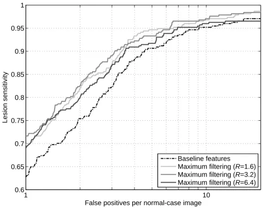
The results of the performed comparisons are listed in Tables 2.3 to 2.5. In these tables, the second column shows the mean sensitivity obtained by the approach given in the first column, the third column shows the approach with which the current one is compared, and for each comparison, thep-value is given in the fourth column. Significant differences are shown in bold. The FROC curves yielded by the compared approaches are shown in Figures 2.4 to 2.6.

2.5 Discussion

The results in Table 2.3 indicate that the proposed method for feature maxima prop-agation led to a significant improvement over the unprocessed features utilized as the baseline in this study. For instance, using a neighborhood with a radius of 1.6 mm, the maximum filtering algorithm increased the mean sensitivity from 0.926 to 0.953 in the range from 3.5 to 15 FPs/image. This increase in sensitivity corresponds to a substan-tial decrease of 36.5% in the number of masses missed during candidate detection. We expect that this will lead to a substantial improvement of the overall sensitivity when subsequent refinement steps, such as false positive reduction, are added. Taking into account a particular operating point such as 4 FPs/image, which can be considered a typical choice in order to maximize the performance of those subsequent steps while min-imizing the candidate complexity, the improvement is even larger (0.882 versus 0.931)

(35)

Table 2.3. Mean sensitivity (S) achieved by the mass candidate detection system provided with features with and without maximum filtering (baseline features)

Feature set S Compared with p-value

Baseline features 0.926 – –

Maximum filtering (R= 1.6) 0.953 Baseline features <0.0002 Maximum filtering (R= 3.2) 0.953 Baseline features 0.0022 Maximum filtering (R= 6.4) 0.940 Baseline features 0.1156

Table 2.4. Mean sensitivity (S) achieved by the mass candidate detection system when the ensemble of neural networks, the gentle adaboost classifier and the random forest classifier are applied for image location classification

Classifier S Compared with p-value

Neural networks (5 networks) 0.926 – –

Gentle adaboost (100 stumps) 0.934 Neural networks (5 networks) 0.0418 Random forest (100 trees) 0.948 Neural networks (5 networks) 0.0002 Gentle adaboost (100 stumps) 0.0008

Table 2.5. Mean sensitivity (S) achieved by the mass candidate detection system when the maximum-filtered features and the random forest classifier are applied independently or together

Detection with S Compared with p-value

N. nets. + max. filt. (R = 1.6) 0.953 – –

R. forest + baseline feat. 0.948 – –

R. forest + max. filt. (R = 1.6) 0.958 N. nets. + baseline feat. <0.0002 N. nets. + max. filt. (R = 1.6) 0.0748 R. forest + baseline feat. 0.0098

and accounts for a 41.5% reduction of missed masses.

The results in Table 2.3 also give an insight into the effect of using increasing neigh-borhood radii during maxima propagation. While with the smallest radii of 1.6 and 3.2 mm the obtained mean sensitivities were the highest, using larger radii, such as 6.4 mm and above, significantly deteriorated detection performance. A possible expla-nation is that, with those increasing radii, more normal image locations, that meant to have mismatched features due to their normal condition, were randomly matched with spurious peaks. As a consequence, they became as suspicious as true lesions for the clas-sifier and resulted in false-positive detections. This brings into consideration the point stated in Section 2.3.2 about selecting a compromise value for the neighborhood radius.

(36)

2.5 Discussion 29 1 10 0.6 0.65 0.7 0.75 0.8 0.85 0.9 0.95 1

False positives per normal-case image

Lesion sensitivity

Baseline features

Maximum filtering (R=1.6)

Figure 2.4. FROC curves for the mass candidate detection system provided with features with and without maximum filtering (baseline features).

1 10 0.6 0.65 0.7 0.75 0.8 0.85 0.9 0.95 1

Lesion sensitivity

Neural networks (5 networks) Gentle adaboost (100 stumps) Random forest (100 trees)

Figure 2.5. FROC curves for the mass candidate detection system using the ensemble of neural networks, the gentle adaboost classifier and the random forest classifier for image location classification.

(37)

30 Mass candidate detection 1 10 0.6 0.65 0.7 0.75 0.8 0.85 0.9 0.95 1

Lesion sensitivity

Neural networks (5 networks)

Neural networks + maximum filtering (R=1.6)

Random forest + baseline features

Random forest + maximum filtering (R=1.6)

Figure 2.6. FROC curves for the mass candidate detection system when the maximum-filtered features and the random forest classifier are applied independently or together.

Given our experimental results for this particular CAD application, a value of 1.6 mm is preferred, as it yielded virtually the same mean sensitivity as using 3.2 mm (with even a lower p-value when comparing with the baseline features) and is expected to introduce less distortion.

Considering our random forest-based method, similar trends as in the previous ex-periment were observed (see Table 2.4). In this case, the mean sensitivity increased from 0.926 to 0.948, which corresponds to a 29.7% reduction of missed masses. Due to its relation with the proposed random forest classifier, the gentle adaboost classification method was evaluated as well. The results in Table 2.4 indicate that this method also led to an improvement over the ensemble of neural networks, although it was not significant. This improvement can be explained by the weighting mechanism used during training. Since the weights associated with the feature vectors are modified by the algorithm, the training set used at each iteration can be regarded as a different set with a different prevalence for each feature vector, which results in a similar feature vector resampling approach as the one taken by random forests. Actually, when error estimates for the feature vectors cannot be introduced as part of the adaboost learning procedure, resam-pling of the original training set according to the assigned weights is suggested. Thus, under the conditions given in our problem, the feature selection process carried out by the stumps over the modified training sets is expected to give a certain improvement,