A score test of homogeneity in generalized additive models for zero-inflated count data

(1)

A Score Test of Homogeneity in Generalized Additive Models for

Zero-Inflated Count Data

by

GAOWEI NIAN

B.S., Henan University, China, 2012

A REPORT

submitted in partial fulfillment of the

requirements for the degree

MASTER OF SCIENCE

Department of Statistics

College of Arts and Sciences

KANSAS STATE UNIVERSITY

Manhattan, Kansas

2014

Approved by: Major Professor Wei-Wen Hsu

(2)

Copyright

GAOWEI NIAN

(3)

Abstract

Zero-Inflated Poisson (ZIP) models are often used to analyze the count data with excess zeros. In the ZIP model, the Poisson mean and the mixing weight are often assumed to depend on covariates through regression technique. In other words, the effect of covariates on Poisson mean or the mixing weight is specified using a proper link function coupled with a linear predictor which is simply a linear combination of unknown regression coefficients and covariates. However, in practice, this predictor may not be linear in regression pa-rameters but curvilinear or nonlinear. Under such situation, a more general and flexible approach should be considered. One popular method in the literature is Zero-Inflated Gen-eralized Additive Models (ZIGAM) which extends the zero-inflated models to incorporate the use of Generalized Additive Models (GAM). These models can accommodate the non-linear predictor in the link function. For ZIGAM, it is also of interest to conduct inferences for the mixing weight, particularly evaluating whether the mixing weight equals to zero. Many methodologies have been proposed to examine this question, but all of them are de-veloped under classical zero-inflated models rather than ZIGAM. In this report, we propose a generalized score test to evaluate whether the mixing weight is equal to zero under the framework of ZIGAM with Poisson model. Technically, the proposed score test is developed based on a novel transformation for the mixing weight coupled with proportional constraints on ZIGAM, where it assumes that the smooth components of covariates in both the Pois-son mean and the mixing weight have proportional relationships. An intensive simulation study indicates that the proposed score test outperforms the other existing tests when the mixing weight and the Poisson mean truly involve a nonlinear predictor. The recreational fisheries data from the Marine Recreational Information Program (MRIP) survey conducted

(4)

by National Oceanic and Atmospheric Administration (NOAA) are used to illustrate the proposed methodology.

(5)

List of Figures

4.1 Observed proportion of the number of fish caught per hour per individual. . 21

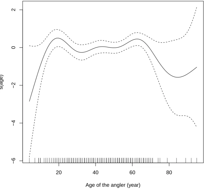
4.2 Plot of the smooth function components of the Poisson mean, on the log scale, of the fitted ZIGAM with the recreational fisheries data. . . 22

(8)

List of Tables

4.1 Empirical sizes and powers of score test statistics for different forms of ω_i∗

with Poisson mean µ∗_i = exp(0.5−0.25xi), at 5 % significant level. . . 16

4.2 Empirical sizes and powers of score test statistics for different forms of ω_i∗

with Poisson mean µ∗_i = exp(0.5−0.3m(xi)), at 5 % significant level. . . 17

4.3 Observed score test statistics and the associated p-values for heterogeneity in recreational fisheries data . . . 19

(9)

Acknowledgments

First of all, I would like to thank my major professor, Dr. Wei-Wen Hsu, for all his guidance, suggestions and encouragement.

I would also like to thank Dr. Weixin Yao and Dr. Christopher Vahl for their willingness to serve on my committee and for their valuable insight.

Finally, I would like to thank my parents, my brother and my sister for their support and endless love and I would also like to thank my wife for her encouragement during my graduate education. In addition, I will thank everyone who helped me during the completion of the report.

(10)

Chapter 1 Introduction

The Zero-Inflated Poisson (ZIP) regression model is a simple two-component mixture model that is often used for count data containing many zeros. In the ZIP model, one

component occurring with the probability ω is a degenerate distribution with mass one at

zero, while the other component occurring with the probability (1−ω) is a standard Poisson

distribution with the mean µ(see, for example, Lambert, 1992).

Under this classical ZIP model, the effect of covariates on the Poisson mean and the mix-ing weight is specified by a proper link function (such as log link; logit link function) coupled with a linear predictor which is simply a linear combination of unknown regression coeffi-cients and covariates. However, in practice, this predictor may not be linear in regression parameters but curvilinear or nonlinear. In other words, the observed features of the data may not be consistent with the ZIP model. For example, in the paper of Lam et al (2006), they found that age had a nonlinear effect on the outcome variable, the number of days of missed primary activities in a given period. In the paper of Liu and Chan (2011), they found that sampling (Julian) day had a nonlinear effect on the outcome variable, jellyfish catch per unit. For such a problem where the predictor is not linear, one popular method called Zero-Inflated Generalized Additive Models (ZIGAM) which extended the zero-inflated models to incorporate the use of Generalized Additive Models (GAM) has been discussed widely (See,

(11)

for example, Barry and Welsh, 2002; Ma et al., 2010). These models can accommodate the nonlinear predictor in the link function.

As a goodness-of-fit test, it is also of interest to evaluate whether the mixing weight in the ZIGAM equals to zero. But the revelent methodologies are all developed under classical ZIP models rather than ZIGAM (see, for example, Jansakul and Hinde, 2002; Todem et al., 2012). To our knowledge, there is no test for homogeneity under the framework of ZIGAM. In this report, we propose a generalized score test to evaluate whether the mixing weight equals to zero under the frame work of ZIGAM, focusing on the Poisson model. Technically, the proposed approach is developed based on the novel transformation proposed by Todem et al. (2012) and an assumption used by Ma et al. (2010). Their assumption assumes that the smooth components of covariates in the Poisson mean and the mixing weight have proportional relationships. In fact, ZIGAM coupled with this assumption is called Constrained Zero-Inflated Generalized Additive Models (COZIGAM) (Liu and Chan, 2011). In sum, the proposed test is developed under the framework of COZIGAM. A resam-pling approach proposed by Lin et al. (1994) is adopted to characterize the null limiting distribution of our test statistic.

This report is organized as follows. In chapter 2, we briefly introduce the ZIP model and the COZIGAM. In chapter 3, the proposed score test based on the approach of Todem et al. (2012) is discussed here as well as the resampling skill. In chapter 4, the performances of the proposed score test are compared to those of the existing score tests (Jansakul and Hinde, 2002 and Todem et al. 2012). Also, a recreational fisheries data set is used to illustrate the proposed methodology. Finally, some conclusions are provided in chapter 5.

(12)

Chapter 2 Costrained Zero-Inflated Generalized

Additive Models

2.1 Zero-inflated Poisson Model

Assume that yi, i= 1,· · · , n, are counts from a ZIP model and xi = (xi1, xi2,· · · , xip)

0

is the correspondingp×1 vector of covariates. The probability mass function of the mixture model is P r(Yi =yi) =      ωi+ (1−ωi) exp{−µi}, if yi=0, (1−ωi) exp{−µi}µyii yi! , if yi >0. , (2.1)

where µi is the mean of the standard Poisson distribution and ωi is known as the mixing

weight. In the ZIP model, the zeros are generated from two different components: a de-generate distribution with mass one at zero and a standard Poisson distribution with mean

µi. The first component occurs with the probability ωi and produces only zeros, while the

second component occurs with the probability (1−ωi) (Jansakul and Hinde, 2002). Lambert

(13)

functions are, respectively, logµi =x 0 iβ and log ωi 1−ωi =g0_iγ,

where xi and gi are covariate vectors and β, γ are t× 1 and r ×1 vectors of unknown

parameters. In equation(2.1), generally the mixing weightsωi are constrained in an interval,

−exp{−µi}/(1−exp{−µi})6ωi 61, i=1,...,n. (2.2)

Since the mixing weightωi can be either negative, zero or positive, the corresponding models

are Zero-Deflected Poisson, standard Poisson and Zero-Inflated Poisson, respectively (Dietz and B¨ohning, 2000).

2.2 Constrained Zero-inflated Generalized Additive

Mod-els

Generalized Additive Models (Hastie and Tibshirani, 1990; Wood, 2006) have been used widely in the literature to incorporate nonlinear predictors in Zero-Inflated models (See, for example, Barry and Welsh, 2002; Ma et al., 2010). It is more flexible to use GAM in a formal analysis due to the smooth terms.

In general, the Poisson means and the mixing weights in the ZIP model have the following structures, gµ(µi) = x 0 iβ and gω(ωi) = g 0 iγ,

whereµi is the Poisson mean; ωi is the proportion of the extra zeros; the gµ(·) and gω(·) are

link functions for the Poisson mean and mixing weight, which are often assumed to be log and logit link functions, respectively, under ZIP.

(14)

Under the framework of Zero-Inflated Generalized Additive Models, the more general structures for the Poisson means and the mixing weights can be assumed as,

gµ(µi) = β0+ p X j=1 sj(xij), and gω(ωi) =α0+ p X j=1 hj(xij),

whereβ0 andα0 are unknown parameters;sj(·) andhj(·) are smooth functions which can be

estimated by the penalized likelihood approach (See, for example, Green Peter J., 1987; Liu et al. 2012). Actually, the penalized likelihood estimator of sj generally equals to Q linear

combination of certain basis functions. In other words, the smooth function evaluated at

xi could be expressed as Diξ, where Di is the ith row of the design matrix D of the basis functions, and ξ is the parameter vector to be estimated.

Here we also assume that some covariates affect the mixing weight and the nondegenerate

distribution mean proportionally on the link scales (Liu and Chan, 2011). Under this

assumption, the models have fewer unknown parameters and thus can be more accurately estimated (Ma et al., 2010). Specially, we assume

hj =δsj.

ZIGAM coupled with this assumption is called Constrained Zero-Inflated Generalized Ad-ditive Model (COZIGAM) (Liu and Chan, 2011). Under COZIGAM, the structures for the means of the nondegenerate distribution and the mixing weights become:

gµ(µi) = β0+ p X j=1 sj(xij), and gω(ωi) =α0+δ p X j=1 sj(xij),

(15)

Chapter 3 Main framework

3.1 Testing Hypotheses

As a goodness-of-fit test, one is often interested in the two-sided hypotheses,

H0 :ωi = 0, for all i vs. Ha :ωi 6= 0, for some i, (3.1)

where ωi satisfies the constraints in equation (2.2). To test these hypotheses, a suitable

natural transformation (Todem et al., 2012) of ωi that incorporates covariates should be

considered. The natural transformation is then given by,

ωi = πi−exp{−µi} 1−exp{−µi} , 0≤πi ≤1. (3.2) where, πi = exp(−exp(x 0 iγ))and µi = exp(x 0 iβ).

(16)

Based on the transformation in equation (3.2), the hypotheses (3.1) are formally represented as,

H0 :πi = exp{−µi}, for all i vs. Ha :πi 6= exp{−µi}, for some i.

If a suitable parameterization of πi is considered, the homogeneity hypothesis above is

reduced to a problem involving a small number of parameters (See, Todem et al., 2012). We already know that the Poisson means under GAM have the following form,

µi = exp{β0+

p

X

j=1

sj(xij)}.

Given the natural transformation and the proportional constraints on the GAM with zero-inflated data, the quantity πi is assumed to be,

πi = exp{−exp{α0+δ

p

X

j=1

sj(xij)}}.

We assume the following reparameterization, γ=β0−α0. Then πi = exp{−exp{β0 −γ+

δPp

j=1sj(xij)}}. After the reparameterization, the new hypotheses are given,

H0 :γ = 0 andδ = 1 vs. Ha:γ 6= 0 or δ6= 1. (3.3)

3.2 Score test under COZIGAM

In classical parametric estimation, the unknown parameters are commonly estimated by maximum likelihood. However, for estimating GAMs, penalized likelihood method pro-vides more powerful tools (Wood, 2000). For observations y1,...,yn, the penalized likelihood

(17)

function is given by ``(θ(β0, ξ), γ, δ, λ) =`(θ(β0, ξ), γ, δ)− 1 2λξ 0 Kξ = n X i=1 I(yi = 0) log(πi) +I(yi >0) log (1−πi) exp{−µi}µyii (1−exp{−µi})yi! −1 2λξ 0 Kξ, where K = (K1,K2, . . . ,Kq, . . . ,KQ) 0

is the penalty matrix in which Kq is a 1 ×Q

vector; λ is the smoothing parameter corresponding to the penalty term, which controls

the trade-off between the smoothness of the function and goodness-of-fit. The smoothing parameter can be selected by generalized cross-validation (GCV). Since the score test only requires the penalized likelihood estimates of the parameters under the null hypothesis, the general score test only involves fitting the standard Poisson model with GAM for the mean. Based on the above penalized likelihood function and the link function for Poisson meanµi

and ωi, the score vector is

S(θ(β0, ξ), γ, δ) =       Sθ(θ(β0, ξ), γ, δ) Sγ(θ(β0, ξ), γ, δ) Sδ(θ(β0, ξ), γ, δ)       =       ∂``(θ(β0,ξ),γ,δ) ∂θ ∂``(θ(β0,ξ),γ,δ) ∂γ ∂``(θ(β0,ξ),γ,δ) ∂δ       , where ∂`` ∂β0 = n X i=1 I(yi=0)log(πi) +I(yi>0) −πilog(πi) 1−πi +I(yi>0) yi−µi− µiexp (−µi) 1−exp (−µi) ,

(18)

∂`` ∂ξq = n X i=1 I(yi=0)log(πi) +I(yi>0) ₋ πilog(πi) 1−πi δ p X j=1 sjq(xij) + I(yi>0) yi−µi − µiexp (−µi) 1−exp (−µi) p X j=1 sjq(xij) −λKqξ 0 , q = 1, . . . , Q, ∂`` ∂γ = ∂l ∂πi ∂πi ∂γ = n X i=1 −I(yi=0)log(πi) +I(yi>0) πilog(πi) 1−πi , ∂`` ∂δ = ∂l ∂µi ∂µi ∂δ = n X i=1 I(yi=0)log(πi)−I(yi>0) πilog(πi) 1−πi p X i=1 sj(xij) .

The expected information matrix I(θ(β0, ξ), γ, δ) can be partitioned as

I(θ(β0, ξ), γ, δ) =       Iθ(θ(β0, ξ), γ, δ) Iθγ(θ(β0, ξ), γ, δ) Iθδ(θ(β0, ξ), γ, δ) Iγθ(θ(β0, ξ), γ, δ) Iγ(θ(β0, ξ), γ, δ) Iγδ(θ(β0, ξ), γ, δ) Iδθ(θ(β0, ξ), γ, δ) Iδγ(θ(β0, ξ), γ, δ) Iδ(θ(β0, ξ), γ, δ)       ,

where the elements Iθ,Iθγ=I

0

γθ, Iθδ=I

0

δθ, Iγ,Iγδ=Iδγ and Iδ are, respectively,

−E h ∂2_l₍_θ₍_β 0,ξ),γ,δ) ∂θ∂θ0 i , −E h ∂2_l₍_θ₍_β 0,ξ),γ,δ) ∂θ∂γ0 i , −E h ∂2_l₍_θ₍_β 0,ξ),γ,δ) ∂θ∂δ0 i , −E h ∂2_l₍_θ₍_β 0,ξ),γ,δ) ∂γ2 i , −E h ∂2_l₍_θ₍_β 0,ξ),γ,δ) ∂γ∂δ0 i , −E h ∂2_l₍_θ₍_β 0,ξ),γ,δ) ∂δ2 i .

(19)

Under the null hypothesis, the general score statistic is then

Sω =S

0

γ,δ(ˆθ(β0, ξ),0,1)Λ−1Sγ,δ(ˆθ(β0, ξ),0,1),

where ˆθ(β0,ξ) is the maximum penalized likelihood estimator (MPLE) under the null model

and the MPLE has asymptotically normality (see, Liu and Chan, 2011); and

Sγ,δ(ˆθ(β0, ξ),0,1) =     Pn i=1 I(yi=0)(ˆµi)−I(yi>0) ˆ µiexp (−µî) 1−exp (−µî) Pn i=1 h −I(yi=0)(ˆµi) +I(yi>0) ˆ µiexp (−µî) 1−exp (−µî) i Pp j=1sj(xij)     , Λ =I_γ,δ∗ (ˆθ(β0, ξ),0,1)−Iγ,δ,θ∗ (ˆθ(β0, ξ),0,1)Iθ−1(ˆθ(β0, ξ),0,1)I∗ 0 θ,γ,δ(ˆθ(β0, ξ),0,1), where I_γ,δ∗ (ˆθ(β0, ξ),0,1) =    Iγ(ˆθ(β0, ξ),0,1) Iγδ(ˆθ(β0, ξ),0,1) Iδγ(ˆθ(β0, ξ),0,1) Iδ(ˆθ(β0, ξ),0,1)   , I_γ,δ,θ∗ (ˆθ(β0, ξ),0,1) =    Iγθ(ˆθ(β0, ξ),0,1) Iδθ(ˆθ(β0, ξ),0,1)   , I_θ,γ,δ∗ (ˆθ(β0, ξ),0,1) = Iθγ(ˆθ(β0, ξ),0,1) Iθδ(ˆθ(β0, ξ),0,1) .

As we mentional in previous chapter, we assume that µi=exp{β0+Pp_j₌₁sj(xij)} and πi=

exp{−exp{β0−γ+δ

Pp

j=1sj(xij)}}. Under the null model, given that γ=0, δ=1 coupled

with ˆθ(β0,ξ) which is the estimate of θ(β0,ξ), estimates of entries of the information matrix

(20)

Iθγ(ˆθ(β0, ξ),0,1) =            Pn i=1 −µî2exp (−µî) 1−exp (−µî) Pn i=1 −µî2exp (−µî) 1−exp (−µî) Pp j=1sj1(xij) .. . Pn i=1 −µî2exp (−µî) 1−exp (−µî) Pp j=1sjQ(xij)            , Iθδ(ˆθ(β0, ξ),0,1) =            Pn i=1 ˆ µi2exp (−µî) 1−exp (−µî) Pp j=1sj(xij) Pn i=1 ˆ µi2exp (−µî) 1−exp (−µî) Pp j=1sj(xij) Pp j=1sj1(xij) .. . Pn i=1 ˆ µi2exp (−µî) 1−exp (−µî) Pp j=1sj(xij) Pp j=1sjQ(xij)            , Iγ(ˆθ(β0, ξ),0,1) = n X i=1 ˆ µi2exp (−µî) 1−exp (−µî) , Iγδ(ˆθ(β0, ξ),0,1) = n X i=1 − µî 2_{exp (−}_µ_ˆ i) 1−exp (−µî) p X j=1 sj(xij) , Iδ(ˆθ(β0, ξ),0,1) = n X i=1 ˆ µi2exp (−µî) 1−exp (−µî) p X j=1 sj(xij) p X j=1 sj(xij) .

This term Iθ(ˆθ(β0, ξ),0,1) can be obtained by an R program (See detailed information in

Appendix B)

3.3 Resampling method

We’d like to use a resampling approach which applies the idea of Lin et al. (1994) to approximate the empirical distribution of the proposed score statistic. This resampling technique has been used widely in the literature (for example, Zhu and Zhang, 2006). In addition, this resampling approach can save a lot of time, compared with a simple

(21)

nonpara-metric bootstrap (Efron and Tibshirani, 1993).

Before applying the resampling approach, we need to make some basic preparation. Under the null model, we define ci,

ci =bi(ˆθ(β0, ξ),0,1)−Iθγδ∗ ∗I

−1

θ ∗ai(ˆθ(β0, ξ),0,1).

The function ci can be obtained from a Taylor expansion of bi(ˆθ(β0, ξ),0,1).

Actually, bi(θ(βo, ξ), γ, δ) andai(θ(βo, ξ), γ, δ) are the score functions under the null model,

they are, respectively,

bi(ˆθ(βo, ξ),0,1) =Sγ,δ(ˆθ(β0, ξ),0,1),

ai(ˆθ(βo, ξ),0,1) =

∂``(ˆθ(β0, ξ),0,1)

∂θ .

And I_θγδ∗ and Iθ can be acquired can be obtained from the fisher information matrix,

I_γδθ∗ =    Iγθ(ˆθ(β0, ξ),0,1) Iδθ(ˆθ(β0, ξ),0,1)   =     Pn i=1 −µî2exp (−µî) 1−exp (−µî) Pn i=1 ˆ µi2exp (−µî) 1−exp (−µî) Pp i=1sj(xij)     , Iθ =Iθ(ˆθ(β0, ξ),0,1).

Then we randomly generate {ε(₁b),· · · , ε(nb)} independently from standard normal

distribu-tion, where superscript (b) stands for replications,b=1,· · · , B. Given the realizations of the data, {yi, xi}ni=1, and values of γ = 0, δ = 1, we calculate the statistic U

(b)

n (ˆθ(β0, ξ),0,1) =

Pn

i=1ci ∗ε (b)

i , where θˆ is the maximum penalized likelihood estimator of θ under the null

model. Then we calculate the proposed score statistic for artificial observations

S_ω(b_n) = (U_n(b)(ˆθ(β0, ξ),0,1)) 0

(22)

By repeatedly generating the normal variates {ε1,· · · , εn} for B times, and repeating

the above procedure for each generated sample, we obtain the empirical distribution ofSω(b),

b=1,· · · , B. The asymptotical p-value of the test is the proportion of times the artificial score statistics which are greater than or equal to the observed test statistic SO given the generated data {yi, xi}ni=1. Thenp-value=B−1

PB

b=11{S (b)

(23)

Chapter 4 Numerical study

4.1 Simulation

The simulation study is aimed to evaluate the empirical performance of the score test under COZIGAM. We assess the performances of our proposed score test to those of the score tests proposed by Jansakul and Hinde (2002) and Todem et al. (2012). In our simula-tions, data are generated from a mixture model with true mixing weightsω_i∗ and a Poisson distribution with two different forms of true mean: one depends on covariates through re-gression technique, µ∗_i=exp(0.5−0.25xi), where xi is a covariate generated from a uniform

distribution on the interval(0,1); the other one depends on smooth functions of covariates,

µ∗_i=exp(0.5−0.3m(xi)), where m(xi)=(0.2x11i (10(1−xi))6 + 10(10xi)3(1−xi)10)/8. The

score test of Jansakul and Hinde (2002) assumed that ωi=γ0 +γ1xi, and that of Todem et

al. (2012) assumed that ωi=(πi−exp(−µi))(1−exp(−µi))−1 andπi=exp(−exp(γ0+γ1xi))

under the alternative hypothesis. For our proposed score test under COZIGAM, we assume that ωi=(πi −exp(−µi))(1−exp(µi))−1 under the alternative, where πi=exp{−exp{β0 −

γ+δPp

j=1sj(xij)}} and µi=exp(β0+

Pp

j=1sj(xij)). With the assumption and

(24)

H0: γj=0, j=0, 1, for the test of Jansakul and Hinde (2002); and H0: γj=βj, j=0, 1, for

the test of Todem et al. (2012). For each simulation, we have 1000 replicates for sample size 50, 100, 200 and 400.

(25)

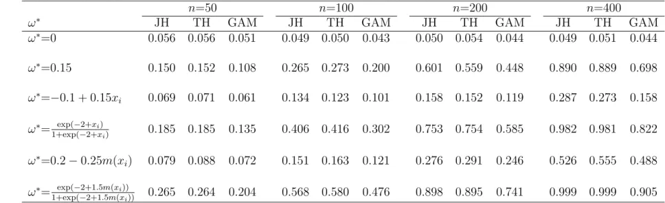
Table 4.1: Empirical sizes and powers of score test statistics for different forms of ω∗_i with Poisson mean µ∗_i = exp(0.5− 0.25xi), at 5 % significant level.

n=50 n=100 n=200 n=400

ω∗ JH TH GAM JH TH GAM JH TH GAM JH TH GAM

ω∗=0 0.056 0.056 0.051 0.049 0.050 0.043 0.050 0.054 0.044 0.049 0.051 0.044 ω∗=0.15 0.150 0.152 0.108 0.265 0.273 0.200 0.601 0.559 0.448 0.890 0.889 0.698 ω∗=−0.1 + 0.15xi 0.069 0.071 0.061 0.134 0.123 0.101 0.158 0.152 0.119 0.287 0.273 0.158 ω∗= exp(−2+xi) 1+exp(−2+xi) 0.185 0.185 0.135 0.406 0.416 0.302 0.753 0.754 0.585 0.982 0.981 0.822 ω∗=0.2−0.25m(xi) 0.079 0.088 0.072 0.151 0.163 0.121 0.276 0.291 0.246 0.526 0.555 0.488 ω∗= exp(−2+1.5m(xi)) 1+exp(−2+1.5m(xi)) 0.265 0.264 0.204 0.568 0.580 0.476 0.898 0.895 0.741 0.999 0.999 0.905 Note: 1. xi a covariate taking onnuniformly distributed values on (0,1),m(xi)=(0.2x11i (10(1−xi))6+ 10(10xi)3(1−xi)10)/8; 2. JH stands

for the score test of Jansakul and Hinde, TH stands for the score test of Todem et al., GAM stands for the score test under COZIGAM; 3. For each simulation, we have 1000 replicates.

(26)

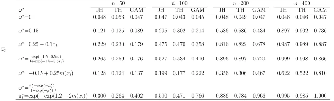
Table 4.2: Empirical sizes and powers of score test statistics for different forms of ω∗_i with Poisson mean µ∗_i = exp(0.5− 0.3m(xi)), at 5 % significant level.

n=50 n=100 n=200 n=400

ω∗ JH TH GAM JH TH GAM JH TH GAM JH TH GAM

ω∗=0 0.048 0.053 0.047 0.047 0.043 0.045 0.048 0.049 0.047 0.048 0.046 0.047 ω∗=0.15 0.121 0.125 0.089 0.295 0.302 0.214 0.586 0.586 0.434 0.897 0.902 0.736 ω∗=0.25−0.1xi 0.229 0.230 0.179 0.475 0.470 0.358 0.816 0.822 0.678 0.987 0.989 0.887 ω∗= exp(−1.5+0.5xi) 1+exp(−1.5+0.5xi) 0.265 0.259 0.176 0.527 0.534 0.410 0.896 0.897 0.720 0.999 0.998 0.866 ω∗=−0.15 + 0.25m(xi) 0.128 0.124 0.137 0.199 0.177 0.222 0.356 0.306 0.467 0.622 0.522 0.810 ω∗=π∗i−exp (−µ ∗ i) 1−exp (−µ∗ i) , π_i∗=exp(−exp(1.2−2m(xi)) 0.300 0.264 0.402 0.590 0.471 0.766 0.886 0.784 0.966 0.995 0.985 1.000

Note: 1. xi a covariate taking on n uniformly distributed values on (0,1), m(xi)=(0.2x11i (10(1−xi))6+ 10(10xi)3(1−xi)10)/8; 2. JH stands for

the score test of Jansakul and Hinde, TH stands for the score test of Todem et al., GAM stands for the score test under COZIGAM; 3. For each simulation, we have 1000 replicates.

(27)

4.2 Findings from simulation

Firstly, the three tests have controlled type I error rates well (Table 4.1 and Table 4.2). In Table 4.1, the true Poisson means depend on covariates through regression technique. The results demonstrate that no matter whether the true mixing weight is constant, a linear form of covariate, or smooth function of covariate, our proposed score test loses some efficiency, compared to the other two tests.

However, in Table 4.2, the true Poisson mean depends on smooth functions of covariate. It is clear that our proposed test outperforms the other two tests when the true mixing weights are, ω∗_i=−0.15 + 0.25m(xi) and ω∗i=

π_i∗−exp(−µ∗_i) 1−exp(−µ∗

i) , where π

∗

i=exp(exp(1.2−2m(xi)).

This is expected as data were generated under the situation where the ture mixing weights and the true Poisson means involve smooth functions of covariate.

Finally, incorporating smooth functions can improve the performances of the score test. Our proposed approach is indeed more powerful in detecting heterogeneity in the population when nonlinear covariates effects exist in both the Poisson mean and the mixing weight. Besides, our proposed approach loses some efficiency when the Poisson mean or the mixing weight truly depends on a linear function of covariates, on the link scales. However, the true model is always unknown to the analyst, it is a more conservative strategy to use our proposed score test to conduct inference for the mixing weight.

4.3 Application to Recreational Fisheries data

National Oceanic and Atmospheric Administration (NOAA) have conducted several fish-ing surveys since 2004. The main goal of these surveys is workfish-ing with both commercial and recreational fishermen to count what’s being caught, when, where, and how. They mainly use the collected information to decide how many fish can be taken recreationally and commercially without having negative effect on the sustainability of individual fisheries.

(28)

Table 4.3: Observed score test statistics and the associated p-values for heterogeneity in recreational fisheries data

Response

Methodology test statistic p-vlaue

Test of Jansakul and Hinde 28.6527 0.016

Test of Todem et al. 28.7641 0.017

Test under COZIGAM 22.2899 0.009

The information also ensures appropriate measures are taken to recover fisheries in trouble. To illustrate our methodology, we used fisheries data collected during July and August of 2013. The primary count outcome is the number of fish caught per hour per individual (NFPHPI). Age of the angler is considered as the covariate. After looking at the original data, we can observe many zeros in the data (see Figure 4.1). This implies that there may exist extra zeros. We evaluated the homogeneity hypothesis using the proposed score test under ZIGAM with Poisson, given the evidence from Figure 4.2 that there is nonlinear relationship between the age of angler (year) and the predictor in the Poisson mean on the log link scale. The nondegenerate distribution is a standard Poisson regression model with mean

µi=exp(β0+s(Age)) and the mixing weightωi is given by equation (3.2) with the quantity

πi=exp(−exp(β0 −γ +δs(Age))). The score test of Jansakul and Hinde (2002) and that

proposed by Todem et al. (2012) were also conducted. With the above parameterizations, the null hypotheses to be evaluated become: H0: γ=0, and δ=1, for our score test; H0:

γj=0, j=0, 1, for Jansakul and Hinde’s test; H0: γj=βj, j=0, 1, for test of Todem et al.

The first two tests were conducted by replacing the nuisance parameter β by its maximum

likelihood estimate under the null distribution, while our proposed test was conducted by

replacing the nuisance parameterθ by its maximum penalized likelihood estimate under the

null distribution. Results of this analysis are given in Table 4.3.

The results in Table 4.3 show that all the three tests reject the homogeneity hypothesis at 5 % significance level. But our proposed test is more powerful to detect the heterogeneity

(29)

(30)

Number of fish caught per hour per individual Propor tion 0 2 4 6 8 10 0.0 0.2 0.4 0.6 0.8 1.0

(31)

20 40 60 80 −6 −4 −2 0 2

Age of the angler (year)

s(age)

Figure 4.2: Plot of the smooth function components of the Poisson mean, on the log scale, of the fitted ZIGAM with the recreational fisheries data.

(32)

Chapter 5 Discussion

In this report, we proposed a generalized score test to evaluate the mixing weight under zero-inflated generalized additive models. Simulation studies indicate that our proposed test loses some efficiency compared with the tests of Jansakul (2002) and Todem et al. (2012) when the true Poisson mean depends on a linear form of covariates. However, if both the Poisson mean and the mixing weight truly involve smooth functions of covariates, our proposed test outperforms the other tests. Because the true model is always unknown to the analyst, we suggest that it is a conservative strategy to evaluate the mixing weight with our proposed score test.

It is worth nothing that, Wald test will be a good candidate to evaluate whether the mixing weight equals to zero under COZIGAM if the alternative model can be fitted in routine. In the literature, the R package ”COZIGAM” was developed to fit the alternative model, but it has been removed from the CRAN list in R software due to its non-stability. Furthermore, it is also worthwhile to extend our approach to analyze the longitudinal/-correlated data using random effects models or generalized estimating equations approach. These are actually the subjects of future research.

(33)

Bibliography

[1] Lambert D. Zero-inflated poisson regression, with an application to defects in manu-facturing. Technometrics, 34(1), 1992.

[2] Lam K. F., Xue H. Q., and Cheung Y. B. Semiparametric analysis of zero-inflated count data. Biometrics, 62:996–1003, 2006.

[3] Liu H. and Chan K. S. Generalized additive models for zero-inflated data with partial constraints. Scandinavian Journal of Statistics, 38:650–665, 2011.

[4] Barryand S. C. and Welsh A. H. Generalized additive modelling and zero inflated count data. Ecological Modelling, 157:179–188, 2002.

[5] Ma S., Liu A., Carr J., Post W., and Kronmal R. Statistical modeling of agatston score in multi-ethnic study of atherosclerosis (mesa). PLoS ONE, 5:e12036, 2010.

[6] Jansakul N. and Hinde J. P. Score tests for zero-inflated poisson models.Computational Statistics & Data Analysis, 40:75–96, 2002.

[7] Todem D., Hsu W-W., and Kim K. M. On the efficiency of score tests for homogeneity in two-component parametric models for discrete data. Biometrics, 68:975–982, 2012. [8] Lin D. Y., Fleming T. R., and Wei L. J. Confidence bands for sruvival curves under

the proportional hazards model. Biometrika, 81:73–81, 1994.

[9] Dietz E. and B¨ohning D. On estimation of the poisson parameter in zero-modified

(34)

[10] Hastie T. and Tibshirani R. Generalized additive models.Statistical Science, 1:297–318, 1986.

[11] Wood S. N. Generalized Additive Models, An Introduction with R., volume 1st Ed.

London: Chapman and Hall, 2006.

[12] Green P. J. Penalized likelihood for general semi-parametric regression models. Inter-national Statistical Review, 55:245–259, 1987.

[13] Liu H., Ma S., Kronmal R., and Chan K. S. Semiparametric zero-inflated modeling in multi-ethnic study of atherosclerosis (mesa). The Annals of Applied Statistics, 6(3): 1236–1255, 2012.

[14] Wood S. N. Modelling and smoothing parameter estimation with multiple quadratic penalties. J. R. Statist. Soc. B, 62:413–428, 2000.

[15] Zhu Z. Y. and Zhang H. Spatial sampling design under the in?ll asymptotic framework.

Enrironmetrics, 17:323–337, 2006.

[16] Efron B. and Tibshirani R. J. An Introduction to the Bootstrap. New York: Chapman

(35)

Appendix A

Second derivative of the Penalized

likelihood function

∂2_l₍_θ₍_β 0, ξ), γ, δ) ∂θ∂γ0 =            Pn i=1 −I₍_y_i₌₀₎logπi+I(yi>0) _π

i(logπi)2+πilogπi−πi2logπi (1−πi)2 Pn i=1 h −I(yi=0)logπi+I(yi>0)

πi(logπi)2+πilogπi−πi2logπi (1−πi)2 i Pp j=1sj1(xij) .. . Pn i=1 h −I(yi=0)logπi+I(yi>0)

πi(logπi)2+πilogπi−πi2logπi (1−πi)2 i Pp j=1sjQ(xij)            , ∂2l(θ(β0, ξ), γ, δ) ∂θ∂δ0 =            Pn i=1 h −I(yi=0)logπi+I(yi>0) _π

i(logπi)2+πilogπi−πi2logπi (1−πi)2 i Pp j=1sj(xij) Pn i=1 h −I₍_y_i₌₀₎logπi+I(yi>0) _π

i(logπi)2+πilogπi−πi2logπi (1−πi)2 i Pp j=1sj(xij)Ppj=1sj1(xij) .. . Pn i=1 h −I₍_y_i₌₀₎logπi+I(yi>0) _π

i(logπi)2+πilogπi−πi2logπi (1−πi)2 i Pp j=1sj(xij)Ppj=1sjQ(xij)            , ∂2l(θ(β0, ξ), γ, δ) ∂γ∂γ0 = n X i=1 I(yi=0)logπi −I(yi>0)

πi(logπi)2 +πilogπi−πi2logπi

(1−πi)2

(36)

∂2l(θ(β0, ξ), γ, δ) ∂γ∂δ0 = n X i=1 −I(yi=0)logπi+I(yi>0)

πi(logπi)2+πilogπi−πi2logπi

(1−πi)2 p X j=1 sj(xij) , ∂2l(θ(β0, ξ), γ, δ) ∂δ∂δ0 = n X i=1 I(yi=0)logπi−I(yi>0)

πi(logπi)2+πilogπi−πi2logπi

(1−πi)2 p X j=1 sj(xij) !2 .

(37)

Appendix B

Code

rm(l i s t=l s(a l l=TRUE ) ) ;l i b r a r y( mgcv ) ;l i b r a r y( b o o t ) ; ########################################################### N1=1000; ## MC s a m p l e s N2=1000; ## r e s a m p l i n g s a m p l e s a0 = 0 . 5 ; a1 =−0.25; ## t r u e p a r a m e t e r s o f P o i s s o n mean d e p e n d i n g on x3 #a0 = 0 . 5 ; a1 =−0.3; ## t r u e p a r a m e t e r s o f P o i s s o n mean d e p e n d i n g on s 1 i t e r a t i o n =100; ## show t h e p r o g r e s s e v e r y x x x i n t e r a t i o n s . ########################################################### f o r ( n i n c( 4 0 0 , 2 0 0 , 1 0 0 , 5 0 ) ){ ptm=Sys .time( ) ; S1=numeric( 0 ) S2=numeric( 0 ) S3=numeric( 0 ) f o r(mc i n 1 : N1 ) { ########################################################### ##G e n e r a t i n g P o i s s o n d a t a ( s a m p l e s i z e n ) i =1 s e q 0=numeric( 0 ) while( i<=n ) { j =0 s e q 0 1=numeric( 0 )

(38)

x3=r u n i f( 1 , 0 , 1 )

s 1 = ( 0 . 2∗x3 ˆ11∗( 1 0∗(1−x3 ))ˆ6+10∗( 1 0∗x3 ) ˆ 3∗(1−x3 ) ˆ 1 0 )/8 u=exp( a0+a1∗x3 ) ;#u=e x p ( a0+a1∗s 1 ) ;

p=0 x=r u n i f( 1 , 0 , 1 ) cp=p+(1−p )∗exp(−u )∗( u ˆ ( 0 ) )/( f a c t o r i a l ( 0 ) ) while( cp<=x ) { py=(1−p )∗exp(−u )∗( u ˆ ( j +1))/( f a c t o r i a l ( j +1)) cp=cp+py j=j +1 } s e q 0 1=c( s e q 0 1 , j , u , x3 , i ) z=c( s e q 0 1 ) s e q 0=c( s e q 0 , z ) i=i +1 mat=matrix( s e q 0 , 4 ) mat=t(mat) }##end o f g e n e r a t i n g P o i s s o n d a t a y=mat[ , 1 ] x3=mat[ , 3 ] mmat=data.frame( y , x3 ) ; #################################################### #s c o r e t e s t f o r GAM

f i t 1 =gam ( y˜s ( x3 ) ,family=” p o i s s o n ” ) x1=predict( f i t 1 , t y p e=” t e r m s ” ) s s=predict( f i t 1 , t y p e=” l p m a t r i x ” ) lambdahat =( f i t 1$s p ) ˆ 2 ;

S= f i t 1$sm [ [ 1 ] ] [ 1 2 ] [ [ 1 ] ] [ [ 1 ] ]

c o e f n e w 1=matrix(c( f i t 1$ c o e f[ 1 ] , 1 ) ,nrow=2 ,ncol=1) X1=matrix(c(matrix( 1 , n , 1 ) , x1 ) ,nrow=n ,ncol=2) muhat1=exp( X1%∗%c o e f n e w 1 )

#s c o r e t e s t s t a t i s t i c

I 0 0=as.matrix( vcov ( f i t 1 ) )

I 0 1=sum(−muhat1 ˆ2∗exp(−muhat1 )/(1−exp(−muhat1 ) ) ) I 0 2=sum( muhat1 ˆ2∗exp(−muhat1 )/(1−exp(−muhat1 ) )∗x1 ) I 1 1=sum(−muhat1 ˆ2∗exp(−muhat1 )/(1−exp(−muhat1 ) )∗s s [ , 2 ] )

(39)

I 1 2=sum( muhat1 ˆ2∗exp(−muhat1 )/(1−exp(−muhat1 ) )∗( s s [ , 2 ]∗x1 ) ) I 2 1=sum(−muhat1 ˆ2∗exp(−muhat1 )/(1−exp(−muhat1 ) )∗s s [ , 3 ] ) I 2 2=sum( muhat1 ˆ2∗exp(−muhat1 )/(1−exp(−muhat1 ) )∗( s s [ , 3 ]∗x1 ) ) I 3 1=sum(−muhat1 ˆ2∗exp(−muhat1 )/(1−exp(−muhat1 ) )∗s s [ , 4 ] ) I 3 2=sum( muhat1 ˆ2∗exp(−muhat1 )/(1−exp(−muhat1 ) )∗( s s [ , 4 ]∗x1 ) ) I 4 1=sum(−muhat1 ˆ2∗exp(−muhat1 )/(1−exp(−muhat1 ) )∗s s [ , 5 ] ) I 4 2=sum( muhat1 ˆ2∗exp(−muhat1 )/(1−exp(−muhat1 ) )∗( s s [ , 5 ]∗x1 ) ) I 5 1=sum(−muhat1 ˆ2∗exp(−muhat1 )/(1−exp(−muhat1 ) )∗s s [ , 6 ] ) I 5 2=sum( muhat1 ˆ2∗exp(−muhat1 )/(1−exp(−muhat1 ) )∗( s s [ , 6 ]∗x1 ) ) I 6 1=sum(−muhat1 ˆ2∗exp(−muhat1 )/(1−exp(−muhat1 ) )∗s s [ , 7 ] ) I 6 2=sum( muhat1 ˆ2∗exp(−muhat1 )/(1−exp(−muhat1 ) )∗( s s [ , 7 ]∗x1 ) ) I 7 1=sum(−muhat1 ˆ2∗exp(−muhat1 )/(1−exp(−muhat1 ) )∗s s [ , 8 ] ) I 7 2=sum( muhat1 ˆ2∗exp(−muhat1 )/(1−exp(−muhat1 ) )∗( s s [ , 8 ]∗x1 ) ) I 8 1=sum(−muhat1 ˆ2∗exp(−muhat1 )/(1−exp(−muhat1 ) )∗s s [ , 9 ] ) I 8 2=sum( muhat1 ˆ2∗exp(−muhat1 )/(1−exp(−muhat1 ) )∗( s s [ , 9 ]∗x1 ) ) I 9 1=sum(−muhat1 ˆ2∗exp(−muhat1 )/(1−exp(−muhat1 ) )∗s s [ , 1 0 ] ) I 9 2=sum( muhat1 ˆ2∗exp(−muhat1 )/(1−exp(−muhat1 ) )∗( s s [ , 1 0 ]∗x1 ) ) I 2 2 2=sum( muhat1 ˆ2∗exp(−muhat1 )/(1−exp(−muhat1 ) ) )

I 2 3 2=sum(−muhat1 ˆ2∗exp(−muhat1 )/(1−exp(−muhat1 ) )∗x1 ) I 3 2 2=t( I 2 3 2 )

I 3 3 2=sum( muhat1 ˆ2∗exp(−muhat1 )/(1−exp(−muhat1 ) )∗x1∗x1 )

sgama1=sum( muhat1∗( ( y==0)∗1)−(( y>0)∗1 )∗( muhat1∗exp(−muhat1 )/(1−exp(−muhat1 ) ) ) )

s d e l t a 1=sum((−muhat1∗( ( y==0)∗1 ) + ( ( y>0)∗1 )∗( muhat1∗exp(−muhat1 )/(1−exp(−muhat1 ) ) ) )∗x1 ) S c o r e 1=matrix(c( sgama1 , s d e l t a 1 ) ,nrow=2 ,ncol=1)

C11=matrix(c( I 2 2 2 , I 2 3 2 , I 3 2 2 , I 3 3 2 ) ,nrow=2 ,ncol=2)

C12=matrix(c( I 0 1 , I 0 2 , I 1 1 , I 1 2 , I 2 1 , I 2 2 , I 3 1 , I 3 2 , I 4 1 , I 4 2 , I 5 1 , I 5 2 , I 6 1 , I 6 2 , I 7 1 , I 7 2 , I 8 1 , I 8 2 , I 9 1 , I 9 2 ) , nrow=2 ,ncol=10) C13=t( C12 ) C1=C11−C12%∗%I 0 0%∗%C13 s t s 1=t( S c o r e 1 )%∗%s o l v e( C1 )%∗%S c o r e 1 s t s 1=c( s t s 1 ) ##s t s 1 i s t h e o b s e r v e d s c o r e s t a t i s t i c f o r Gam. ############################################################################# ##R e s a m p l i n g f o r GAM #r e s a m p l i n g s e t up s c o r e a 1 0=−muhat1+y

(40)

s c o r e a 1 2 =(−muhat1+y )∗s s [ , 3 ]−matrix( lambdahat∗S [ 2 , ]%∗%t(t( f i t 1$ c o e f[ 2 : 1 0 ] ) ) , n , 1 ) s c o r e a 1 3 =(−muhat1+y )∗s s [ , 4 ]−matrix( lambdahat∗S [ 3 , ]%∗%t(t( f i t 1$ c o e f[ 2 : 1 0 ] ) ) , n , 1 ) s c o r e a 1 4 =(−muhat1+y )∗s s [ , 5 ]−matrix( lambdahat∗S [ 4 , ]%∗%t(t( f i t 1$ c o e f[ 2 : 1 0 ] ) ) , n , 1 ) s c o r e a 1 5 =(−muhat1+y )∗s s [ , 6 ]−matrix( lambdahat∗S [ 5 , ]%∗%t(t( f i t 1$ c o e f[ 2 : 1 0 ] ) ) , n , 1 ) s c o r e a 1 6 =(−muhat1+y )∗s s [ , 7 ]−matrix( lambdahat∗S [ 6 , ]%∗%t(t( f i t 1$ c o e f[ 2 : 1 0 ] ) ) , n , 1 ) s c o r e a 1 7 =(−muhat1+y )∗s s [ , 8 ]−matrix( lambdahat∗S [ 7 , ]%∗%t(t( f i t 1$ c o e f[ 2 : 1 0 ] ) ) , n , 1 ) s c o r e a 1 8 =(−muhat1+y )∗s s [ , 9 ]−matrix( lambdahat∗S [ 8 , ]%∗%t(t( f i t 1$ c o e f[ 2 : 1 0 ] ) ) , n , 1 ) s c o r e a 1 9 =(−muhat1+y )∗s s [ , 1 0 ]−matrix( lambdahat∗S [ 9 , ]%∗%t(t( f i t 1$ c o e f[ 2 : 1 0 ] ) ) , n , 1 ) s c o r e a 1=cbind( s c o r e a 1 0 , s c o r e a 1 1 , s c o r e a 1 2 , s c o r e a 1 3 , s c o r e a 1 4 , s c o r e a 1 5 , s c o r e a 1 6 , s c o r e a 1 7 , s c o r e a 1 8 , s c o r e a 1 9 )

s c o r e a l=t( s c o r e a 1 )

s c o r e w 1=cbind( X1 [ , 1 ]∗( ( ( y==0)∗1 )∗muhat1−(( y>0)∗1 )∗( ( muhat1∗exp(−muhat1 ) )/(1−exp(−muhat1 ) ) ) ) , X1 [ , 2 ]∗(−(( y==0)∗1 )∗muhat1 +(( y>0)∗1 )∗( ( muhat1∗exp(−muhat1 ) )/(1−exp(−muhat1 ) ) ) ) )

s c o r e w 1=t( s c o r e w 1 ) Iwa1=C12 I a 1=I 0 0 c i 1=s c o r e w 1−Iwa1%∗%I a 1%∗%t( s c o r e a 1 ) ##r e s a m p l i n g s e q 1=matrix( , 1 , N2 ) f o r ( k i n 1 : N2 ) { e 1=matrix(rnorm( n , 0 , 1 ) , n , 1 ) u1=c i 1%∗%e 1 s b 1=t( u1 )%∗%s o l v e( C1 )%∗%u1 s b 1=c( s b 1 ) s e q 1 [ 1 , k ]= s b 1 } p1=mean( ( s e q 1>s t s 1 )∗1 ) E1=(p1<0 . 0 5 )∗1 S1=c( S1 , E1 )

##end o f r e s a m p l i n g f o r GAM and S1 a r e t h e r e s a m p l i n g s c o r e s t a t i s t c s f o r Gam #######################################################

#s c o r e t e s t s t a t i s t i c o f JH

#f i n d t h e MLE o f b e t a under s t a n d a r d p o i s s o n .

f i t 2 =glm( y˜x3 , family=” p o i s s o n ” ) ; c o e f 2= f i t 2$ c o e f;

(41)

G2=matrix(c(matrix( 1 , n , 1 ) , x3 ) ,nrow=n ,ncol= 2 ) ; muhat2=exp( X2%∗%c o e f 2 ) ;

D2=diag(c( muhat2 ) ) ;

#s c o r e t e s t s t a t i s t i c

s c o r e 2=t(G2)%∗%( ( ( y==0)∗1−exp(−muhat2 ) )/exp(−muhat2 ) ) ; s c o r e 2 1=t( X2 )%∗%(−(( y==0)∗1 )∗muhat2 +(( y>0)∗1 )∗( y−muhat2 ) ) ; f 1 1=t( X2 )%∗%D2%∗%X2 ;

f 2 2=t(G2)%∗%diag(c(((1−exp(−muhat2 ) )/exp(−muhat2 ) ) ) )%∗%G2 ; f 2 1=t(G2)%∗%diag(c(−muhat2 ) )%∗%X2 ; f 1 2=t( f 2 1 ) ; C2=f 2 2−f 2 1%∗%s o l v e( f 1 1 )%∗%f 1 2 ; s t s 2=t( s c o r e 2 )%∗%s o l v e( C2 )%∗%s c o r e 2 ; s t s 2=c( s t s 2 ) ; ##s t s 2 i s t h e o b s e r v e d s c o r e s t a t i s t i c f o r JH ######################################################### #r e s a m p l i n g f o r J a n s a k u l #r e s a m p l i n g s e t up

s c o r e a 2=cbind( X2 [ , 1 ]∗(−muhat2 +(( y>0)∗1 )∗y ) , X2 [ , 2 ]∗(−muhat2 +(( y>0)∗1 )∗y ) ) s c o r e a 2=t( s c o r e a 2 )

s c o r e w 2=cbind(G2 [ , 1 ]∗( ( y==0)∗1−exp(−muhat2 ) )/exp(−muhat2 ) , G2 [ , 2 ]∗( ( y==0)∗1−exp(−muhat2 ) )/exp(−muhat2 ) )

s c o r e w 2=t( s c o r e w 2 )

Iwa2=t(G2)%∗%diag(c(−muhat2 ) )%∗%X2 I a 2=t(G2)%∗%diag(c( muhat2 ) )%∗%X2 c i 2=s c o r e w 2−Iwa2%∗%s o l v e( I a 2 )%∗%s c o r e a 2 ##R e s a m p l i n g s e q 2=matrix( , 1 , N2 ) f o r(m i n 1 : N2 ) { e 2=matrix(rnorm( n , 0 , 1 ) , n , 1 ) u2=c i 2%∗%e 2 s b 2=t( u2 )%∗%s o l v e( C2 )%∗%u2 s b 2=c( s b 2 ) s e q 2 [ 1 ,m]= s b 2 } p2=mean( ( s e q 2>s t s 2 )∗1 ) E2=(p2<0 . 0 5 )∗1

(42)

S2=c( S2 , E2 ) ########################################################## # TH’ s s c o r e t e s t s t a t i s t i c ##f i n d t h e MLE o f b e t a under s t a n d a r d p o i s s o n . f i t 3 =glm( y˜x3 , family=” p o i s s o n ” , data=mmat) c o e f 3= f i t 3$ c o e f

X3=matrix(c(matrix( 1 , n , 1 ) , x3 ) ,nrow=n ,ncol=2) muhat3=exp( X3%∗%c o e f 3 )

##s c o r e t e s t s t a t i s t i c o f TH

D3=diag(c( muhat3 ) )

s c o r e 3=t( X3 )%∗%( muhat3∗( ( ( ( y==0)∗1)−exp(−muhat3 ) )/(1−exp(−muhat3 ) ) ) ) ; s c o r e 3 1=t( X3 )%∗%(−muhat3 +(( y>0)∗1 )∗y )

H11=t( X3 )%∗%D3%∗%X3 ;

H22=t( X3 )%∗%diag(c( ( ( muhat3 ) ˆ 2 )∗exp(−muhat3 )/(1−exp(−muhat3 ) ) ) )%∗%X3 ; H12=t( X3 )%∗%diag(c(−(( muhat3 ) ˆ 2 )∗exp(−muhat3 )/(1−exp(−muhat3 ) ) ) )%∗%X3 ; H21=t( H12 ) ; C3=H22−H21%∗%s o l v e( H11 )%∗%H12 ; s t s 3=t( s c o r e 3 )%∗%s o l v e( C3 )%∗%s c o r e 3 ; s t s 3=c( s t s 3 ) ##s t s 3 i s t h e o b s e r v e d s c o r e s t a t i s t i c f o r TH. ########################################################### #r e s a m p l i n g f o r TH

s c o r e a 3=cbind( X3 [ , 1 ]∗(−muhat3 +(( y>0)∗1 )∗y ) , X3 [ , 2 ]∗(−muhat3 +(( y>0)∗1 )∗y ) ) s c o r e a 3=t( s c o r e a 3 )

s c o r e w 3=cbind( X3 [ , 1 ]∗muhat3∗( ( ( ( y==0)∗1)−exp(−muhat3 ) )/(1−exp(−muhat3 ) ) ) , X3 [ , 2 ]∗muhat3∗( ( ( ( y==0)∗1)−exp(−muhat3 ) )/(1−exp(−muhat3 ) ) ) )

s c o r e w 3=t( s c o r e w 3 )

Iwa3=t( X3 )%∗%diag(c(−muhat3 ˆ2∗exp(−muhat3 )/(1−exp(−muhat3 ) ) ) )%∗%X3 I a 3=t( X3 )%∗%D3%∗%X3 c i 3=s c o r e w 3−Iwa3%∗%s o l v e( I a 3 )%∗%s c o r e a 3 s e q 3=matrix( , 1 , N2 ) f o r(t i n 1 : N2 ) { e 3=matrix(rnorm( n , 0 , 1 ) , n , 1 ) u3=c i 3%∗%e 3 s b 3=t( u3 )%∗%s o l v e( C3 )%∗%u3 s b 3=c( s b 3 )

(43)

s e q 3 [ 1 ,t]= s b 3 } p3=mean( ( s e q 3>s t s 3 )∗1 ) E3=(p3<0 . 0 5 )∗1 S3=c( S3 , E3 ) i f (mc%%i t e r a t i o n ==0){cat( ” i t e r a t i o n = ” , mc , ” o f ” , N1 , ”\n” )}; ############################################### }##end o f MC gam r=mean( S1 ) ; j h r=mean( S2 ) ; t h r=mean( S3 ) ; d u r a t i o n =( Sys .time()−ptm ) ; cat( ”######################################” , ”\n” ) ; cat( ” Sample s i z e=” , n , ”\n” ) ;

cat( ”####### R e s a m p l i n g ######” , ”\n” ) ; cat( ”GAM=” , gam r , ”\n” ) ;

cat( ”JH=” , j h r , ”\n” ) ; cat( ”TH=” , t h r , ”\n” ) ; print( d u r a t i o n ) ;

cat( ”######################################” , ”\n” ) ;

A score test of homogeneity in generalized additive models for zero-inflated count data