Deep learning for supervised classification

DEEP LEARNING FOR SUPERVISED CLASSIFICATION

1. Introduction

One of the most recent area in the machine learning research is Deep Learning. We can define Deep Learning classification models a class of Machine Learning algorithms that use a cascade of many layers of nonlinear processing units for feature extraction and transformation. Each layer uses the output from the previous layer as input, while the final layer gives the final classification. The model may be supervised or unsupervised.

This is a very general definition, which reminds the structure of a neural networks algorithm. Effectively, a Deep Neural Network (DNN) is an artificial neural network with many hidden layers of units between the input and output layers and millions or billions of parameters. For example, in the “Google Brain” project it was developed a massive neural networks with 1 billion parameters to detect cats inside YouTube videos.

Google, Facebook, Microsoft, Apple, in recent months have been investing in the field of Deep Learning. Google acquired Deep Mind to leverage its expertise in Deep Learning methods. Deep Learning algorithms have been applied successfully to computer vision, automatic speech recognition, natural language processing, audio recognition and bioinformatics.

The key idea of Deep Learning is to combine the best techniques from Machine Learning to build powerful general-purpose learning algorithms. However, we don’t have to commit the mistake of identify Deep Learning models with Neural Networks. Other approaches are possible, with the joint use of several powerful statistical models.

In the next paragraph we introduce the approach of supervised classification with ensemble methods, which combine the predictions of several basic estimators built with one or more given learning algorithms in order to improve accuracy and/or robustness over a single estimator. In particular, Bagging, Boosting, Stacking and a generalization of Stacking are illustrated. In paragraph 3 we show an application to a real classification problem, where the last approach has proved to be very effective.

2. Ensemble methods for classification

Ensemble learning is a machine-learning paradigm where multiple learners are trained to solve the same problem. In contrast to ordinary machine learning approaches, which construct one classification algorithm from training data, ensemble methods construct a set of classification algorithms and combine them. An ensemble contains a number of algorithms, which are usually called base learners: Decision Trees, Neural Networks (NN), Support Vector Machine (SVM) or other kinds of machine-learning algorithms

We can distinguish between:  homogeneous base learners,  heterogeneous base learners.

Typically, an ensemble model is constructed in two steps.

1) A number of base learners are constructed, which can be generated in a parallel style or in a sequential style, where the generation of a base learner has influence on the generation of subsequent learners.

2) The base learners are combined, usually by (weighted) majority voting for supervised classification.

Generally, to get a good ensemble, the base learners should be as more accurate as possible, and as more different as possible. In practice, the diversity of the base learners can be introduced in several ways:

 subsampling the training data,  manipulating the attributes,

 injecting randomness into learning algorithms.

The employment of different base learners and/or different combination schemes leads to different ensemble methods. Statistical properties of the methods and reliability of the results are usually obtained by cross-validation. The optimal ‘tuning’ of the models is obtained by a grid-search approach: the analysis is repeated with parameters taken inside fixed intervals, evaluating the results by cross-validation.

2.1. Bagging, Boosting and Stacking

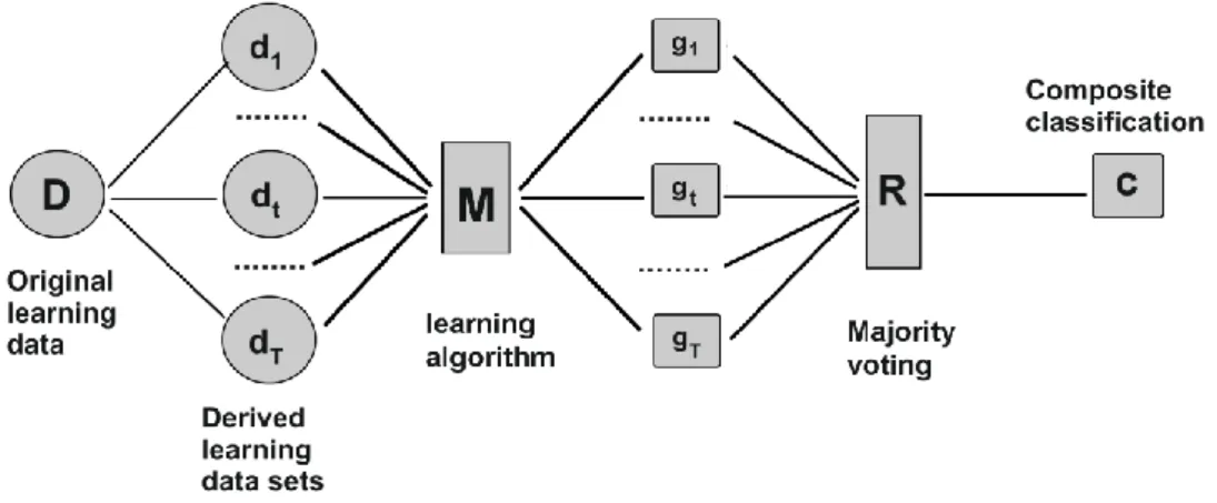
Bagging (Breiman 1996) uses homogeneous learners but different samples of observations and/or predictors (features) to generate different classifiers. To aggregate the classifiers, it is used averaging in regression, majority vote in

classification. The accuracy of the aggregate model is usually not better of the virtual accuracy of the base model, but Bagging reduces the variance and helps to avoid overfitting.

Figure 1– The Bagging (Bootstrap Aggregation) scheme.

Using a single weak learner, Boosting (Schapire 1990), recursively, makes examples currently misclassified more important. This approach, shown in figure 2, is useful for reducing bias, converting weak learners to strong learners, sometimes can give overfitting.

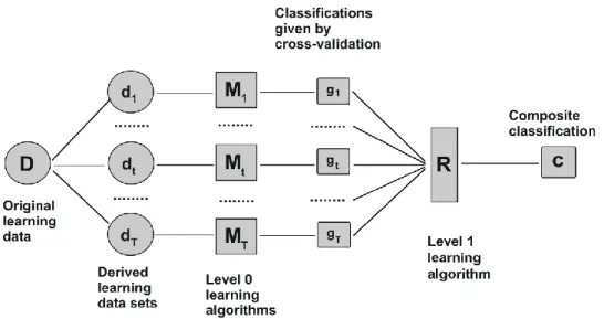
Stacking (Wolpert 1992), unlike bagging and boosting, is not used to combine models of the same type - for example, a set of decision trees. Instead it uses different learning algorithms and two stages.

As shown in figure 3, in level 0 several algorithms are trained on the available data, giving as output the class probabilities for the target, using a cross-validation prediction (usually a 5-fold CV). Then a combiner algorithm is trained on the overall class probabilities to make a final prediction. The goal of the second stage is to combine in the most effective way the predictive capability of the different algorithms of the first stage. From this point of view, it is crucial that the predictive capability is assessed through cross-validation, to avoid to reward the overfitting models. Moreover, this allows to evaluate statistically the individual algorithms that we are using and it is fundamental to make the tuning of the model parameters.

Figure 2– The Boosting scheme.

In real problems, Stacking is less widely used than bagging and boosting. This is because it is computationally demanding, it is difficult to analyze theoretically and because there is no generally accepted best way of doing it - the basic idea can be applied in many different variations.

2.2. Multi-stage Stacking

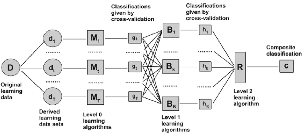
The Stacking approach can be easily generalized to a multi-stage scheme, as shown in figure 4. In this scheme, we added an internal layer with K nodes corresponding to K different models, which elaborates the output of level 0 models. The scheme looks like a feedforward neural network, but with some interesting differences: cross-validation does not allow for overfitting, each node can be a powerful statistical model, the joint use of several different models increases the reliability of the prediction. Many other ensemble methods can be viewed as special cases of stacking in which a data-independent model combination algorithm, such as a majority vote, is used.

Figure 4– Generalized three-stages Stacking

As we mentioned above, we have the problem of choosing the parameters to best tune the algorithms and this requires an evaluation of the algorithm's performance for each set of parameters through cross-validation.

If we have many models with many parameters in several layers, the overall optimization problem is not practically feasible. What is done, is the individual tuning of all algorithms of a layer, starting from the lowest level, and then proceeding to the next layer. Note that each algorithm can be a complex machine-learning method, which may require several hours of processing. Another possibility is to train the models one after another, where each model tries to achieve best results when associated with all the preceding models.

The overall assessment may be carried out again with cross-validation or with the use of an independent data set. With big-data, the data split in training-validation-test sets, is usually enough.

3. An application of Deep Learning

Kaggle is a famous website of Data Science competitions. Any company can obtain a cost-effective way to solve machine-learning problems proposing a competition to the Kaggle’s community of data scientists.

In March 2015, Otto Group, one of the world’s biggest e-commerce companies, proposed one competition. The proposed challenge is the construction of a classification model which is able to accurately classify the products among 9 main product categories, using 93 observed numeric features (obfuscated and with no further information)1. It is a classical supervised classification problem.

The competitors had available one training set with 61678 units which included the category, and a test set with 144368 units without the category. They had to submit a file with the predicted probabilities on the test set, obtaining a score by Kaggle. It was possible to submit a maximum of 3 entries per day. The total prize pool for this competition was $10,000.

As a condition of receipt of the Prize, the winner must deliver the final model’s software code with the associated documentation. The participants in the Otto Group competition were 3848 from all over the world.

The winner model was a generalized 3 stages Stacking model as showed in figure 4. The impressive list of the models used in the first stage is reported in table 1. In level-0 there are 33 models and 8 engineered feature-sets. The cross-validation probability class predictions of these models (plus the engineered feature-sets) are used as meta features for the 2nd stage. The derived features (class probabilities) of the models at the 2nd stage are 33*9=297, the other 8 feature-sets give 148 columns (6*9+1+93) for a total of 445 derived features.

In the 2nd stage (level-1) there are only 3 models: XGboost (Friedman 2000), Neural Networks (NN) and Adaboost (Schapire 1990). The final stage is composed by a weighted mean of the level-1 predictions.

In level-0, there are many different models: Neural Networks, Gradient Boosting (Friedman 2000), RandomForest (Breiman 2001), Logistic Regression, Extremely randomized trees (Geurts et al. 2006), K-Nearest Neighbors (Cover & Hart 1967), Multinomial Naïve Bayes (Zhang 2004), K-means (Hartigan 1975),

1

distributed stochastic neighbor embedding (van der Maaten et al. 2008), Support Vector Machines (Cortes & Vapnik 1995).

Tabella 1 (a) Models used in the first stage of the Stacking model by the winner. M1 RandomForest (R). Dataset= X

M2 Logistic Regression (Scikit). Dataset= Log(X+1) M3 Extra Trees Classifier (Scikit). Dataset= Log(X+1) M4 KNeighborsClassifier (Scikit).

M5 libfm. Dataset= Sparse(X). Each feature value is a unique level. M6 H2O, NN. Bag of 10 runs. Dataset= Sqrt( X + 3/8)

M7 Multinomial Naive Bayes (scikit). Dataset= Log(X+1) M8 Lasagne, NN. Bag of 2 runs.

M9 Lasagne, NN. Bag of 6 runs. Dataset= Scale( Log(X+1) )

M10 sne. Dimension reduction to 3 dimensions. Also stacked 2 kmeans features using the T-sne 3 dimensions.

M11 Sofia. Learner_type="logreg-pegasos" and loop_type="balanced-stochastic". Dataset= Scale(X)

M12 Sofia. Learner_type="logreg-pegasos" and loop_type="balanced-stochastic". Dataset= Scale(X, T-sne Dimension, some 3 level interactions between 13 most important features ) M13 Sofia. Learner_type="logreg-pegasos" and loop_type="combined-roc". Dataset= Log(1+X,

T-sne Dimension, some 3 level interactions between 13 most important features ) M14 Xgboost. Dataset= (X, feature sum(zeros) by row ). Replaced zeros with NA.

M15 Xgboost. Multiclass Soft-Prob. Dataset= (X, 7 Kmeans features with different number of clusters, rowSums(X==0), rowSums(Scale(X)>0.5), rowSums(Scale(X)< -0.5) ) M16 Xgboost. Multiclass Soft-Prob. Dataset= (X, T-sne features, Some Kmeans clusters of X) M17 Xgboost. Multiclass Soft-Prob. Dataset=(X, T-sne features, Some Kmeans clusters of

log(1+X) )

M18 Xgboost. Multiclass Soft-Prob. Dataset=(X, T-sne features, Some Kmeans clusters of Scale(X) )

M19 Lasagne NN(GPU). 2-Layer. Bag of 120 NN runs with different number of epochs. M20 Lasagne NN(GPU). 3-Layer. Bag of 120 NN runs with different number of epochs. M21 XGboost. Trained on raw features. Extremely bagged (30 times averaged). M22 KNN on features X + int(X == 0)

M23 KNN on features X + int(X == 0) + log(X + 1) M24 KNN on raw with 2 neighbours

M25 KNN on raw with 4 neighbours M26 KNN on raw with 8 neighbours M27 KNN on raw with 16 neighbours M28 KNN on raw with 32 neighbours M29 KNN on raw with 64 neighbours M30 KNN on raw with 128 neighbours M31 KNN on raw with 256 neighbours M32 KNN on raw with 512 neighbours M33 KNN on raw with 1024 neighbours

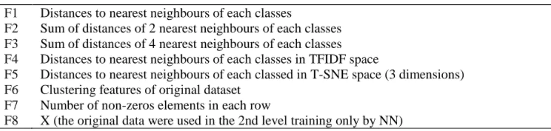
Tabella 1 (b) Models used in the first stage of the Stacking model by the winner. F1 Distances to nearest neighbours of each classes

F2 Sum of distances of 2 nearest neighbours of each classes F3 Sum of distances of 4 nearest neighbours of each classes F4 Distances to nearest neighbours of each classes in TFIDF space

F5 Distances to nearest neighbours of each classed in T-SNE space (3 dimensions) F6 Clustering features of original dataset

F7 Number of non-zeros elements in each row

F8 X (the original data were used in the 2nd level training only by NN)

All the software used in the competition is open source. Lasagne2 is a lightweight library to build and train neural networks. XGboost3 is the Extreme Gradient Boosting. t-SNE4 is the t-Distributed Stochastic Neighbor Embedding. Sofia-ml5 is a library used to obtain Logistic Regression with Pegasos SVM updates. libFM6 is a Factorization Machine Library. H2O7 is a Machine learning library for Python, R, Java. Scikit8 is a machine learning library in Python. In Table 1, the list of models and engineered features is shown. We indicated with X the original dataset with 93 features, with Scale(X) the standardized data, with Sparse(X) the sparse matrix representation of the original data matrix.

Each of the models listed in Table 1 was estimated independently. It does not need a joint estimate that it would almost impossible. Simply, after a tuning step, each model has been applied to the training data, obtaining the estimated probabilities of each class with a k-fold cross-validation. The output of all the models were then put together to create the data set to be analyzed at the level 1. So the stacking model applied does not require extraordinary computational resources and can be built with a traditional PC, even if the long processing time would suggest the use of systems based on GPU. An immediate comment you can make watching the list of Table 1, is that most of the models applied is not specific to the data set analyzed. Essentially, the overall stacking model used in the competition could be applied with excellent performance even in other problems of supervised classification. The estimation of the parameters of the models will change, some models will vary their importance in the final result, but this will be mostly automatic, with light intervention from the researcher. This is exactly the spirit of Deep Learning: build powerful general-purpose learning algorithms. It is worth to 2 _{http://lasagne.readthedocs.org/} 3 _{https://github.com/dmlc/xgboost/tree/master/R-package} 4 _{http://lvdmaaten.github.io/tsne/} 5 _{https://code.google.com/p/sofia-ml/} 6 _{http://www.libfm.org/} 7 _{http://www.H2O.ai} 8 _{http://scikit-learn.org/stable/}

observe that also the runner-up to the competition used a Stacking three-stage scheme, but with a number of models much more reduced.

Another example is the 2009 Netflix competition: this company offered a prize of $1 million for the best model able to recommend new movies to its users, using the handful of movies the users had rated. Data was a sparse matrix with more than 100 million date-stamped movie rating on 17,770 movies by 480,189 users. The solution was an ensemble model with hundreds of predictors and many level-1 learning algorithm (Töscher et al. 2009).

4. Conclusion

Multi-stage Stacking models are very reliable and accurate methods often used in deep learning application. The classification performance of these methods can be very good, sometimes outperforming Deep NN, that, in any case, can be included as one of the models used in Stacking. The strength of this approach is primarily based on the Cross-Validation, that allows an assessment of the reliability of each used model, preventing overfitting. Cross-Validation is the best way to evaluate the prediction error of this kind of composite classifiers. The other distinctive element is the use of several powerful base models, which are estimated to generate a self-adaptable method capable to analyze different sets of data.

Much work is still needed to select the best architecture for multi-stage Stacking and to identify the best mix of models to use, but our impression is that the multi-stage Stacking has classification capabilities that are difficult to reach with other approaches.

References

BREIMAN, L. 2001. Random Forests. Machine Learning Vol. 45, No. 1, pp. 5–32. doi:10.1023/A: 1010933404324.

BREIMAN, L. 1996. Bagging predictors. Machine Learning Vol. 24, No. 2, pp. 123–140. doi:10.1007/BF00058655

CORTES C., VAPNIK, V. 1995. Support-vector networks. Machine Learning Vol. 20, No 3, pp. 273. doi:10.1007/BF00994018.

COVER T.M., HART P.E. 1967. Nearest neighbor pattern classification. IEEE Transactions on Information Theory, Vol.13, No. 1, pp. 21–27.

FRIEDMAN, J. H. 2000. Greedy Function Approximation: A Gradient Boosting Machine. Annals of Statistics, Vol. 29, pp. 1189-1232.

GEURTS P., ERNST. D., AND L. WEHENKEL, 2006. Extremely randomized trees, Machine Learning, Vol. 63, No. 1, pp.3-42.

HARTIGAN, J.A. 1975. Clustering algorithms. John Wiley & Sons, Inc..

NIELSEN, M. A. 2015. Neural Networks and Deep Learning, Determination Press, (http://neuralnetworksanddeeplearning.com/).

RENDLE, S. 2010. Factorization machines. In Proceedings of the 10th IEEE International Conference on Data Mining. IEEE Computer Society.

SCHAPIRE, R. E. 1990. The Strength of Weak Learnability. Machine Learning, Vol. 5, No. 2, pp. 197–227. doi:10.1007/bf00116037

TÖSCHER, A., JAHRER, M., BELL, R.M. 2009. The BigChaos Solution to the Netflix Grand Prize, www.netflixprize.com/assets/GrandPrize2009_BPC_ BigChaos.pdf

VAN DER MAATEN L, HINTON G. 2008. Visualizing data using t-SNE. Journal of Machine Learning Research, Vol. 9, pp. 2579–2605.

WOLPERT, D. 1992. Stacked Generalization. Neural Networks, Vol. 5, No. 2, pp. 241-259.

Zhang, H. 2004. The Optimality of Naive Bayes. FLAIRS2004 conference.

SUMMARY

Deep learning for supervised classification

One of the most recent area in the Machine Learning research is Deep Learning. Deep Learning algorithms have been applied successfully to computer vision, automatic speech recognition, natural language processing, audio recognition and bioinformatics.

The key idea of Deep Learning is to combine the best techniques from Machine Learning to build powerful general‑purpose learning algorithms. It is a mistake to identify Deep Neural Networks with Deep Learning Algorithms. Other approaches are possible, and in this paper we illustrate a generalization of Stacking which has very competitive performances. In particular, we show an application of this approach to a real classification problem, where a three-stages Stacking has proved to be very effective.

_________________________

Agostino DI CIACCIO, Department of Statistics, Univiversity of Rome “La Sapienza”, [email protected]

Giovanni M. GIORGI, Department of Statistics, Univiversity of Rome “La Sapienza”, [email protected]