Proc. IAHS, 371, 83–88, 2015 proc-iahs.net/371/83/2015/ doi:10.5194/piahs-371-83-2015
© Author(s) 2015. CC Attribution 3.0 License.
Open Access
non-stationar
ity
and
e
xtr
apolating
models
to
predict
the
future
(HS02
–
IUGG2015)
Frequency of floods in a changing climate: a case study
from the Red River in Manitoba, Canada
A. Boluwade and P. F. Rasmussen
Department of Civil Engineering, University of Manitoba, Winnipeg, Canada
Correspondence to: P. F. Rasmussen ([email protected])
Received: 17 March 2015 – Accepted: 17 March 2015 – Published: 12 June 2015
Abstract. Spring flooding in the Red River basin is a recurrent issue in the Province of Manitoba, Canada. There have been a number of flood events in recent years and climate change has been suggested as a potential cause. This paper employs a relatively simple model for predicting changes in the frequency distribution of annual spring peak discharge of the Red River as a response to increased GHG concentrations. A regression model is used to predict spring peak flow from antecedent precipitation in the previous fall, winter snow accumulation, and spring precipitation. Data from the Coupled Model Intercomparison Project – Phase 5 (CMIP5) are used to estimate changes in the predictor variables and this information is then employed to derive flood distributions for future climate conditions. Most climate models predict increased precipitation during winter months but this trend is partly offset by a shorter snow accumulation period and higher winter evaporation rates. The means and medians of an ensemble of 16 climate models do not suggest a particular trend toward more or less frequent floods of the Red River. However, the ensemble range is relatively large, highlighting the difficulties involved in estimating changes in extreme events.
1 Introduction
Climate change impacts river flows around the world and is often being linked to severe flood events. The Canadian Prairie region, which includes the provinces of Manitoba, Saskatchewan, and Alberta, has in recent years experienced several major floods that have had a severe impact on people and infrastructure. Many flood events are caused by snow melt in the spring, occasionally exacerbated by rain during the melt period. A significant event on the Red River, dubbed the “flood of the century”, happened in 1997 and affected large parts of Manitoba, North Dakota, and Minnesota. The 1997 Red River flood occurred as a result of an extraordi-narily large snow pack in the basin. Another major event in Manitoba, the 2011 Assiniboine flood, was also the result of a larger-than-normal snow pack.
It is important to gain a better understanding of how cli-mate change may modify flood regimes and extreme events in particular. Such knowledge is critical for the design of new flood protection infrastructure and for flood plain man-agement. Because climate change affects different regions in different ways, such studies must focus on specific river
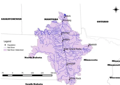
Figure 1.Red River Basin.
2 Methodology
2.1 Study area and data
Most of the Red River basin is located in North Dakota and Minnesota, with only about 15 % of the basin located in Canada, see Fig. 1. The river flows north and crosses the Canada-US border at the city of Emerson. The basin area south of the border is roughly 100 000 km2, and the river is over 800 km long. Most of the basin lies in a glacial lake bed with extremely low relief. This implies that when large flood events occur, they tend to inundate large areas. There have been many historical incidents of flooding in the basin. The most severe event in the past century was the 1997 Red River flood that cost more than CAD 700 million in flood protection measures and damages in Manitoba alone, as well as loss of several lives.. The 1997-event effectively created a large lake, nicknamed the “Red Sea” by locals, with an
esti-mated area of almost 2000 km2. Five percent of Manitoba’s
total farmland was inundated.
The longest continuous record of natural Red River flows is from the hydrometric station at Emerson. The record cov-ers the period from 1913 to present. In most years, the max-imum annual flow occurs in April to early May as a result of snow melt. The primary factors impacting spring floods in the basin are soil moisture at the time of freeze-up in the previous fall, the accumulation of snow during the winter, and rainfall during the melt period. Also of potential impor-tance is the temperature during the melt period and the tim-ing of peak flow in the various tributaries. Warkentin (1999) compiled a set of variables representative of these factors and demonstrated their relationship with spring peak flow at the James Avenue station in Winnipeg. The variables are:
– API (Antecedent Precipitation Index): index of soil
moisture at freeze-up during the previous fall, based on weighted basin precipitation from May to September.
Table 1.Descriptive statistics of the data set used for the regression
analysis.
API MI WP SP TF Q
Mean 2.36 7.51 3.51 0.69 48.15 886.20 Standard Deviation 0.50 3.07 1.11 0.90 16.99 654.22 Range 2.50 15.30 6.75 4.06 69.00 3543.00 Minimum 1.02 2.70 1.85 0.00 12.00 107.00 Maximum 3.52 18.00 8.60 4.06 81.00 3650.00 API=Antecedent Precipitation Index, MI=Melt Index, WP=Winter Precipitation, SP=
Spring Precipitation, TF=Timing Factor.Q=spring peak flow of the Red River at Emerson.
– WP (Winter Precipitation): total average basin
precipi-tation from 1 November of the previous year to the start of active melt (inches).
– SP (Spring Precipitation): total basin precipitation from
the start of active spring melt to the date of the spring crest at Emerson (inches).
– MI (Melt Index): average degree-days per day at Grand
Forks, North Dakota, during the active melt period (in Fahrenheit).
– TF (Timing Factor): an index of the south-north time
phasing of the runoff based on the percentage of trib-utary peaks experienced on the date of the main stem peak at specific points from Halstad to Winnipeg.
Table 1 gives some descriptive statistics of these variables which are available from 1940 to 1999. Warkentin (1999) considered information prior to 1940 to be insufficient for accurate assessment of the variables and the data set has not been updated since 1999. Although more data would have been preferable, the available data are adequate for the methodology used in this study.
2.2 Climate models and future scenarios
The climate model data used in the study were obtained from the Coupled Model Intercomparison Project – Phase 5 (CMIP5) multi-model ensemble (Taylor et al., 2012). A large number of model runs, emission scenarios, time peri-ods, etc. are available. For the purpose of this study, 16 cli-mate models were selected. Additional information about the runs used in this study includes:
– Control climate: Based on the 30-year period from 1971
to 2000.
– Future periods: two periods were considered, the first
from 2031 to 2060, the second from 2071 to 2100.
– Emission scenarios: Two Representative Concentration
Pathways, RCP4.5 and RCP8.5, were considered.
of+4.5 W m−2in year 2010 while RCP8.5 represents the
ra-dioactive forcing of+8.5 W m−2. RCP8.5 is the most severe
of the four scenarios considered in the CMIP5 experiment. The data grids of the different models have resolutions in the order of 1 to 2◦. For each model, the grid point closest to the centroid of the Red River basin south of the Canada-US border was identified. Monthly precipitation, tempera-ture, and evaporation time series for the control and future periods were extracted for each model and each RCP.
2.3 Regression analysis and flood frequency distribution
A regression model can be used to predict spring peak flow from the five predictor variables described in Sect. 2.1. A logarithmic transformation should be used for both spring peak flow and the predictors, in order to better satisfy the requirement of linear regression that the error variance be in-dependent of the predictand and predictors. The model used here is similar to the one employed by Warkentin (1999), ex-cept that he used the discharge at the James Avenue station in Winnipeg rather than at Emerson, and employed nonlin-ear regression to determine the parameters. The regression equation has the following form:
ln(Q)=b0+b1ln(API)+b2ln(WP+SP)+b3ln(MI)
+b4ln(TF)+ε (1)
where, in this study, Qrefers to the spring peak discharge
at Emerson and the other variables are defined in Sect. 2.1. Although not shown here, the annual spring peak discharge is very well fitted by a 2-parameter lognormal distribution.
2.4 Methodology for assessing changes in the distribution of floods
The proposed methodology for assessing change in the dis-tribution of floods is based on the key assumption that the regression model given in Eq. (1) is equally valid in the fu-ture, i.e. that the parameters stay unchanged and that the error variance also does not change. What may change is the distri-bution of predictor variables and the dependent variable. The basic idea is to use climate model data to estimate changes in the distribution of predictor variables and then apply this information to determine changes in the statistics of the de-pendent variable, i.e. the logarithm of spring peak discharge. If a regression model is fitted to a data set (yi, x1i, x2i, . . ., xmi), i=1, . . ., n, by the method of least squares,
then it is well known that the following identities apply:
y= ˆy (2)
and
Sy2=Sy2ˆ+Sε2 (3)
where the hat refers to predicted values and the predictions in this particular case is for the observed predictors, (x1i,
x2i, . . ., xmi), i=1, . . ., n. As usual, an overbar indicates a
sample average andS2indicates a sample variance. The first equation states that the average of predicted values equals the average of observedy-values. The second equation is the well-known analysis-of-variance decomposition, used rou-tinely in tests of regression models. It states that the vari-ance of they variable is equal to the variance of predicted values plus the variance of the error. If a hypothetical future data set of flood peaks and predictor variables were available, one could repeat the regression estimation and would find the same parameters and error variance, apart from the sampling variability always involved in statistical analyses. Therefore, if a future set of predictor variables can be obtained using in-formation from climate models, we can get the mean value and the variance of the dependent variable, in this case the
mean value and variance of ln(Q), using Eqs. (2) and (3).
The mean value and the variance of ln(Q) are the parameters of the 2-parameter log-normal distribution which is known to fit the historical data well.
The critical step in the procedure is the estimation of time series of predictor variables for the future. For this purpose, we make use of the delta-method. Climate model data for current and future climates are used to determine factors of change in the predictor variables. We focus specifically on the three predictor variables API, WP, and SP. The melt-index MI and time melt-index TI are assumed to not change in the future (as discussed in the next section, MI is not even sta-tistically significant in the regression model). The observed time series of predictor variables are scaled using the delta factors to obtain future time series of predictors.
The delta values used as adjustment factors for the three predictor variables are obtained as described below:
– API: The antecedent precipitation index is based on a
weighted average of basin precipitation from May to October (Warkentin, 1999). To calculate the delta value for the API, the following formula is used:
1API= 10 X
i=5
Pfuti −Efuti −Econi
Pconi ωi (4)
where index i refers to calendar month, overbar indicates
mean values,P andEare monthly precipitation and
evapo-ration accumulations from climate models, respectively, and superscripts “fut” and “con” refer to future values and control
period values. The overbars onP andE refer to averaging
over the respective control and future periods. The quantity
ωi is the weight associated with monthiwhich we define as
ωi =k0.5(10−i) (5)
– WP: WP is by definition the total average precipitation
from 1 November to the start of the active melt period. The duration thus varies from year to year, but for the purpose of determining delta factors we ignore year-to-year variations. The following formula is used to calcu-late the delta factors for WP:
1WP=
Pfutwin−Efutwin−Econwin
Pconwin
Dfut
Dcon (6)
where the overbars refer to averages over the winter months
(November to March, averaged over all years), andDrefers
to the average duration of the below-zero period. Information about the below-zero period was derived from the monthly temperature times series from the climate models.
– SP: Delta values for spring precipitation is calculated as
1SP=P fut spring
Pconspring (7)
where the averages are calculated over the months of April and May.
The delta values can be used to construct time series of predictor variables for future climates. This is done by multi-plying the historically observed time series of predictor vari-ables by the corresponding delta values:
APIfut=APIhis×1API (8)
WPfut=WPhis×1WP (9)
SPfut=SPhis×1SP (10)
In summary, the following steps are involved in generating flood distributions for future climates:
1. Determine delta values for the predictor variables API, WP, and SP as described above.
2. Modify the observed time series of API, WP, and SP using the delta values to obtain future time series.
3. Use the future time series of API, WP, and SP along with the remaining predictors as input to the regression
model in Eq. (1) withε set to zero to generate a time
series of ln(Q).
4. Use Eqs. (2) and (3) to determine the mean value and variance of ln(Q).
5. Since from the regression assumptions, ln(Q) has a
normal distribution, the mean value and variance from the previous point represent the parameters of a 2-parameter lognormal distribution of floods in the future climate.
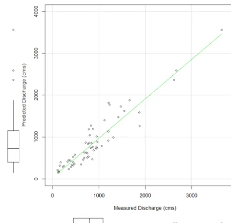
Figure 2.Regression model result.
3 Results
Stepwise regression showed that the variable MI is not sig-nificant in the model and it was therefore not included in the further analysis. The regression model was revised as fol-lows:
ln(Q)=1.925+0.863 ln(API)+1.813 ln(WP+SP)
+0.363 ln(TF)+ε (11)
whereεis assumed to have a zero-mean normal distribution
with constant variance. Figure 2 shows that this assumption is reasonably satisfied. The adjustedR-square value for the above model is 0.83.
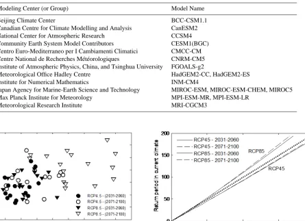
The 16 climate models used in the study are listed in Ta-ble 2. For each of these models, monthly precipitation, evap-oration, and temperature series were extracted for the con-trol period and the two future periods, 2031–2060 and 2071– 2100, corresponding to the RCP4.5 and RCP8.5 scenarios, for the grid point closest to the centroid of the Red River basin. Figure 3 provides a summary of projected changes in annual precipitation and mean annual temperature from the 16 climate models. As expected, all models project increased temperatures, with the later period significantly warmer than the earlier period, and the RCP8.5 scenario generally warmer than the RCP4.5 scenario. By 2100, temperatures could
in-crease by as much as 7–9◦C relative to the control period
em-Table 2.Global climate models from the CMIP5 ensemble used in the study.
Modeling Center (or Group) Model Name
Beijing Climate Center BCC-CSM1.1
Canadian Centre for Climate Modelling and Analysis CanESM2
National Center for Atmospheric Research CCSM4
Community Earth System Model Contributors CESM1(BGC)
Centro Euro-Mediterraneo per I Cambiamenti Climatici CMCC-CM
Centre National de Recherches Météorologiques CNRM-CM5
Institute of Atmospheric Physics, China, and Tsinghua University FGOALS-g2
Meteorological Office Hadley Centre HadGEM2-CC, HadGEM2-ES
Institute for Numerical Mathematics INM-CM4
Japan Agency for Marine-Earth Science and Technology MIROC-ESM, MIROC-ESM-CHEM, MIROC5
Max Planck Institute for Meteorology MPI-ESM-MR, MPI-ESM-LR
Meteorological Research Institute MRI-CGCM3
Figure 3.Changes in mean annual precipitation and mean annual
temperature for the Red River basin as projected by the 16 climate models used in the study.1P is the ratio between the future and the control climate. 1T is the difference between future and control mean temperature in degree Celsius.
phasizes the need to consider many models to adequately ac-count for uncertainties in predictions.
It is worthwhile mentioning that we investigated seasonal changes as well and that most of the increase in annual pre-cipitation appears to be the result of increased winter and spring precipitation while summer and fall precipitation is projected to remain relatively constant, based on the ensem-ble mean. This has important implications for this study.
The methodology outlined in the previous section was used to generate future flood frequency distributions. Rather than presenting the results for each model, each emission sce-nario, and each time period, we have summarized the results in Fig. 4. To create this figure, the assumption was made that for a given emission scenario and a given time period, the 16 model ensemble members are equally likely to represent the future truth. Therefore, each ensemble member is given a probability of 1/16 to be representative of the future. The average of the 16 cumulative distribution functions (CDFs)
Figure 4.Current return periods plotted versus future return periods
of spring peak runoff, as determined by the distributions for control and future climates. See main text for details.
represents the “unconditional” future CDF (for a given RCP and a given time period):
F(x)= 1 16
16 X
i=1
Fi(x) (12)
whereF(x) is the unconditional CDF andFi(x) is the CDF
de-sign for a 110-year flood based on current data if the RCP8.5 scenario is realized.
Figure 4 provides a convenient summary of the results, but hides the fact that there is considerable variation between dif-ferent models. While ensemble averages are useful, it is cru-cial to keep the spread of the ensembles in mind. The ensem-ble spread is a measure of model uncertainty and, depending on the stakes involved, it may be preferable to adopt a more conservative approach when designing important flood pro-tection infrastructure.
4 Conclusions
Estimating the impact of climate change on the distribution of extreme events is difficult for several reasons. Extreme events are by definition rare, so there is usually a limited amount of information available in historical records. Ex-treme events are highly variable in time, resulting in large statistical uncertainties in estimated model parameters. In ad-dition, climate models generally have limitations in simulat-ing extreme weather events. This is particularly true for in-tense, short-duration rainstorms which cannot be simulated realistically in coarse-resolution global climate models.
The present study has focused on the distribution of spring floods in the Red River basin. Spring flooding is a result of a variety of factors, of which the most important is the accumu-lation of snow during the winter season. It is not unable to expect that global climate models will do a reason-able job in simulating basin-wide snow accumulation over the winter season. The basin effectively acts as a spatial and temporal integrator of model output – thereby avoiding some of the issues that are involved in producing extreme events from global climate models.
We have employed a simple regression model to predict spring peak flow in the basin as a function of several pre-dictor variables. The proposed method for assessing climate change impacts uses the well-known delta method to produce scenarios of future predictor variables and this information in turn is used to produce future flood frequency distributions. Results were obtained for several emission scenarios, several future time periods, and for 16 global climate models from the CMIP5 ensemble. The ensemble mean in most cases is relatively close to the historical distribution. However, there is considerable spread in the ensemble, suggesting significant model uncertainty which should be taken into account when designing flood protection work.
Acknowledgements. The global climate model data for this
study were provided by the World Climate Research Programme’s Working Group on Coupled Modelling.
References
Taylor, K. E., Stouffer, R. J., and Meehl, G. A.: An overview of CMIP5 and the experiment design, B. Am. Meteorol. Soc., 93, 485–498, 2012.