Wireless Sensor Network-based Monitoring, Cellular Modelling and Simulations for the Environment

Wireless Sensor Network-based Monitoring, Cellular

Modelling and Simulations for the Environment

Wireless Sensor Networks (WSNs) can be deployed to observe physical phenomena such as pollution,

flooding, insect invasion, and land degradation. Deploying wireless systems are able to overcome

physical constraints such as point to point radio propagation and physical sensing coverage. By building executable cell systems, we have shown that a number of conditions can be evaluated. Examples are line of sight computation and wind or water propagation in complex geographic situations. This paperexplains a method to produce automatically parallel simulators that can be federated later to address the whole problem of deployment design and physical phenomena modelling and simulations.

This work was developed in an international group (SAMES) with the purpose of building and validating tools to ease observation and control aimed at understanding environment evolution and risk reduction.

Key words: Wireless sensor networks, cellular automata, physical modeling, simulation, line of sight, insect invasion, parallel algorithms

IntroductIon

A good knowledge of environmental and physical phenomena will raise awareness of environmental issues that leads to better policies and better participation of citizens. Wireless Sensor Networks (WSNs) are a key technology

for environmental and physical monitoring in a green smart city (OECD 2009) that will allow to a better understanding

of the environment.

A WSN regularly measures values representing the state of a physical system such as water levels for flood

monitoring and CO2 concentration for air pollution. The collected data combined with external knowledge and data (ex. rainfall data, wind data) are then used to monitor, model and simulate the system.

Advances in technology make WSNs an attractive and cost effective proposition. This allows a possible deployment of more sensors, which means having more measurement points and better coverage. The latter increases the precision of a model and simulation.

The problems are how to manage sensor deployments to overcome physical constraints and to get better

coverage. Sensor coverage reflects how well sensors can sense physical phenomena in some locations, and is one

of the metrics used to measure the performance of sensor networks (Wang, B 2011).

1_{Cirela Association, Vélizy, France}

2_{College of Information and Communication Technology, Cantho University, Vietnam} 3_{UBO/Lab-STICC France / Cantho University Vietnam}

4_{Université Gaston BERGER, Senegal}

5_{SAMES stand for Stic Asia Modeling for Environment and Simulation. The actors come from University of Brest Occidental} France (B.Pottier, V.Rodin, B.Nsom, L.Esclade, Raonirivo N Rakoroarijaona), CIRELA Paris (O.Goubier), IRD Paris (S.Stinckwich), Cantho University (HX Huynh, BH Lam ), Hanoi (Vinh), BPPT Jakarta (Udrekh, Hafidz Muslim), DRR Foundation Indonesia (Surono)

Radio signal estimation in a city is critical due to their non-flat characteristics. We cannot predetermine where

the signal goes and what places the signal can be received. It is known that a vague power estimation of the signal

is not enough if the surface is not flat. So it is important to develop tools allowing the estimation of the situation and

the planning of the sensor distribution in the best way possible.

Our research focuses on cellular models to study both physical phenomena and the measurements taken from a WSN in the same geographical area. The location of sensors has an effect on both the effectiveness of the monitoring where correct positions give adequate measurements, and the costs related to the number of sensor nodes necessary for coverage. In a WSN, we have to ensure that the sensors can communicate with their neighbours. Parameters like the coverage area, the communication technology (LoRa, ZigBee,...) and the ground contours are important in this regard.

The next section will present an overview of WSNs, followed by a short introduction on cellular modelling and simulation. An example on the line of sight computation and another example on insect invasion is introduced including the results. This paper concludes with a discussion on current and potential collaborations.

Methodology

Wireless Sensor networks

A WSN consists of sensors, distributed in some areas to measure values representing a state of a physical system. For environment monitoring, this concerns geographically distributed measurements. Furthermore, physical phenomena are dynamic and change with time, which means the periodicity of the measurements is also essential.

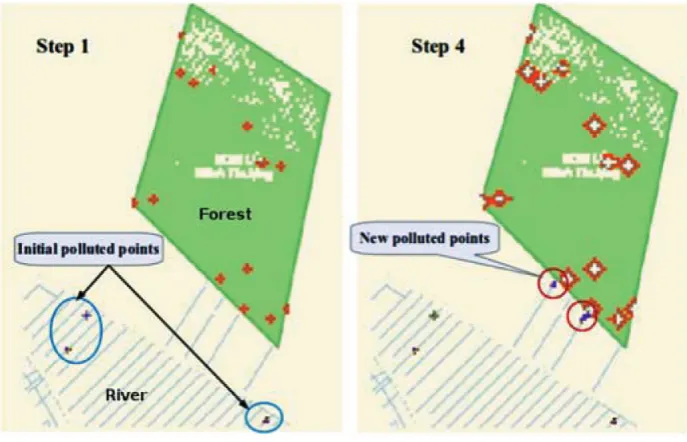
Sensors measure parameters of a physical phenomenon that is being monitored. For example, water pollution in rivers and streams can be monitored by measuring some particularpollutant concentrations in the water. A combination of physical phenomena can be observed and simulated. Figure 1 shows the pollution effects of a forest

fire in a river, where pollutants produced from forest fire could be observed and the phenomena could be simulated

using a WSN (Hoang, VT, 2015).

Figure 1. Two regions marked with red circles representingnew pollution created by the ashes, which were formed from the forest fire.

Measurement data from the sensors are sent to the server via networks. The latter could be in mesh, star, or

hierarchical configurations. Well-known technologies such as GPRS and WiFi can be used. Currently, technologies

like ZigBee, SigFox, LoRa are available for low rate, low power and low cost communication. Cellular companies are also preparing technologies and standards such as cIoT and LTE-M that allow low rate and low power communication (Nokia Networks, 2015).

The collected data are then stored in a database. A complex mathematical model can be used to analyse and

forecast. For example, in the case of flood monitoring, flood forecasting is necessary to warn people in the area in

order to reduce risks, protect property and save lives. External data sources might be needed to complete a model of a physical system, such as weather and topology data for a watershed model. Furthermore, data can also be used to

study flood phenomenon to understand better a flood prone area. Information obtained from the analysis, modelling

and simulation is then disseminated to experts, authorities and the public.

geo-localised cellular Modelling and Simulation

Geo-localised cellular modelling is a very suitable approach to represent physical and environmental phenomena, and their evolution. Important parameters of these phenomena are measured and collected by a WSN, carefully planned, implemented and deployed in the same area as the observed phenomena. The collective measures should cover these phenomena, meaning that cellular modelling can also be used for a WSN deployment to plan some parameters such as sensor locations and number of sensors. Furthermore, the periodicity of the measurements is considered to follow the evolution of the observed phenomena.

A cell in a geo-localised cellular model represents the local state of a physical phenomenon. The system

evolution is based on neighbourhoods defining the communication between cells. There are two most common

neighbourhoods, Von Neumann and Moore (Ilachinski, A 2001). The cells follow a set of rules, applied at each step thus changing the state of the cells whenthe whole system evolves.

UBO/LABSTICC developed PickCell / NetGen, a basic tool allowing the analysis of a geographical zone, in the

form of geo-localised cells in two dimensions. The cells are defined on a browser of maps (Lam et al. 2016, Tran et al. 2016, Iqbal & Pottier 2010, Pottier et al. 2010). The cells can be completed with additional information such as elevation, weather data (GRIB), geological data and land use. The cells allow the computation of radio signals’ line

of sight taking into account the obstacles (elevation). It also allows the prediction of possible water flow through the

slope lines. Figure 2 shows a screenshot of PickCell where latitude, longitude and elevation data are included in the system.

PickCell can generate a program in Occam to be executed as parallel processes, or in CUDA to be executed

on a GPU to accelerate the computation, as well as data needed for the computation. The behaviour of the cells, according to the represented phenomenon, can be added to the simulation.

Some modelling and experimentation have been carried out, for example, Brown Plant Hoppers and the light traps in Mekong Vietnam, as well as wind modelling. In this paper, two examples are presented; a line of sight computation and a desert locust invasion.

caSeS and reSultS

line of sight computation

A good coverage of an observed phenomenon depends not only on the sensors (location, number, precision) but also on the communication technology and deployment area. The topology of the latter, landscape and land-use will constrain radio propagation.

Radio signal propagation can be described as a physical fact or as a logical connectivity between nodes. Several approximations of this propagation can be done, for example by disk modelling coverage for a particular range, by

ray tracing computations, or by line of sight computations. We use this last model to summarise how the flow worked.

Once Space was selected, a cell resolution was chosen (square of 25 by 25 pixels on Figure 2, representing 478 × 478 meters). Not shown is the synthesis of a cell system according to the execution target. We used a Von Neumann N, W, S, E neighbourhood. At this stage, additional data was fetched from servers outside: we added elevation based on each cell’sgeographic position. Simulation programs were produced in a few seconds and then they were bound to a particular behaviour, compiled and executed.

When the physical space description was obtained, we were interested to compute reachable cells in the line of sight from an emitting position. The line of sight represents a ray broadcast in any direction from the emitter. The ray propagation can be stopped by ground topology (hills, valley). Simulation mimics the physical behaviour, by propagating the signal inside a tree rooted at the emitter cell, and covering the Space in concentric circles. Each new

step in the algorithm covered a new circle, and the computation finished in 2× log n steps where n is the number of cells. During ray propagation, the ground profile was collected into routes that were completed progressively based

on positions and elevations. Each cell could decide if the emitter was visible or not by comparing its elevation to the

received profile.

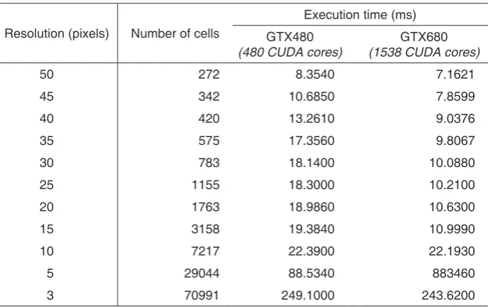
Figure 3. Results of the line of sight computation, accelerated by GPU (Table 1)

In practice, for execution, tools allocate cells on the accelerator and compute channel connectivity. The level of

effective parallelism is high: common GPUs have several hundreds of processors, thus the computations finish at an

impressive speed (see Table 1).

Table 1. Computation time using CUDA (GPU accelerator)

Resolution (pixels) Number of cells

Execution time (ms) GTX480

(480 CUDA cores) (1538 CUDA cores)GTX680

50 272 8.3540 7.1621

45 342 10.6850 7.8599

40 420 13.2610 9.0376

35 575 17.3560 9.8067

30 783 18.1400 10.0880

25 1155 18.3000 10.2100

20 1763 18.9860 10.6300

15 3158 19.3840 10.9990

10 7217 22.3900 22.1930

5 29044 88.5340 883460

desert locust invasion

The research in this area was in collaboration with University Gaston Berger, Senegal and University of North Antsiranana, Madagascar.

Desert locusts change their behaviour, physiology and morphology, in response to density variations. They can exist in two different behavioural phases (Duranton, JF & Lecoq, M 1990): the first one, solitarious where individuals

live in a sparse and scattered manner in recession or remission areas distributed across several Sahel countries

(Uvarov 1977), and they do not venture out of their original habitat and do not affect agricultural production. The

second one, gregarious where individuals are responsible for considerable damage caused to crops with potential

social, ecological and environmental disasters in tropical countries (Herok, CA & Krall, S 1995).

The specificity of desert locusts is that outbreaks happen only within specific conditions, leading to huge swarms, trying to survive by flying to other food sources and escapinge predators. Thus, they migrate from one area to another for better living conditions; and they die if they fail to find a suitable breeding area. Emigration concerns winged individuals who turn to solitarious and then to gregarious before flying in a swarm.

A desert locust can live three to five months depending on the weather and ecological factors. The life cycle hasthree stages: egg, larvae, and adult (Roffey, J & Popov, G 1968). Figure 4 shows five stages, from larvae 1 to

Larvae 5, composing of the larvae phase. In the last stage, a winged transformation occurs and the locustsbecome

mature after some weeks. Mature females can lay eggs if the humidity is sufficient.

The desert locust physical system represents the locust population in their breeding area and their interactions

with weather, vegetation cover and wind, evolving from eggs to adults and flying to other cells, laying eggs.

The physical system is divided in cells; each cell contains eight arrays for eggs, larvae stages 1 to 5, winged, solitarious and gregarious individuals. Each array is subdivided into micro states representing the corresponding individuals’ life cycle period (Traore, M “to appear”).

After some synchronous turns, the neighbours’ cells receive incoming adults of which females can lay eggs three times in their life cycle. This model can be used in population evolution predictions, in time and space. It can also be used in individual number counting.

Figure 4. The lifecycle of a desert locust

Two cases can be considered: the first one is relative to local transitions between micro states in a cell, and the second one is relative to migration between cells. In this paper, the first case that represents the locust life cycle is

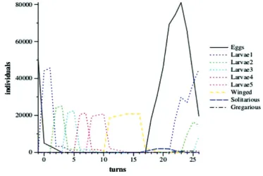
Figure 5 shows the results of a simulation with an initial population of 50000 eggs generated randomly at the

micro state. During the 15 first turns, the population evolves from eggs to winged and solitarious individualsafter 16 turns. A new flow of eggs appears at turn 18, caused by the laying function. The ocust population developed

exponentially with periodic peeks.

Figure 5. Locust population evolution

WSn experIMentatIonS

Two WSN experimentations have been done in collaboration with Indonesia and Vietnam.

A collaboration with BPPT (Agency for the Assessment and Application of Technology) and Diponegoro University

Indonesia has provided results on experiments with sensors monitoring waterways and communicating via Zigbee (Xbee). The maximum distance of communication using Xbee in this experiment was about 500 metres, which was good enough to be used in an urban area.

An experiment using LoRa nodes has been done in Mekong, Vietnam. It shows good results, where LoRa could be used to communicate within a12 -kilometre range.

concluSIonS and dIScuSSIon

Cellular modelling and simulation on environmental and physical phenomena combined with WSN observations are promising approaches to better understand the environment, to reduce environmental and disaster risks, and to live in harmony with environment.

Much work remains to be done, such as the integration of the WSN experimentations, ZigBee and LoRa, with

NetGen/PickCell tools to model, simulate and forecast flooding in urban areas or insects in crop areas.

Suchtechniques have much potential in modelling physical phenomena (flooding, pollution,…) and planning

acknoWledgeMentS

The authors would like to thank University Gaston Berger Senegal and University of North Antsiranana Madagascar for

research collaboration in the desert locust invasion, as well as Diponegoro University Indonesia for the collaboration on WSN for flood monitoring. The SAMES group research is supported in part by the STIC Asia Project.

referenceS

Duranton, JF & Lecoq, M 1990, ’LE CRIQUET PELERIN AU SAHEL’. CIRAD/PRIFAS.

Herok, C A & Krall, S 1995, ‘Economics of desert locust control’. Deutsche Gesellschaft fur Technische Zusammenarbeit (GTZ) GmbH.

Hoang, VT 2015, ‘Cyber-physical systems and mixed simulations’, Master thesis, MRI, UBO.

Ilachinski, A 2001, ‘Cellular Automata, A discrete Universe’, World Scientific Publishing, Singapore.

Iqbal, A & Pottier, B 2010, ‘Meta-simulation of large WSN on multi-core computers’, SpringSim '10 Proceedings of the 2010 Spring Simulation Multiconference, SCS, ACM, Orlando, United States.

Lam, BH & Huynh, HX & Pottier, B 2016, ‘Synchronous networks for bio-environmental surveillance based on cellular automata’, Journal EAI Endorsed Transactions on Context-aware Systems and Applications, vol 16, no 8.

Nokia Networks 2015, LTE-M – Optimizing LTE for the Internet of Things, White Paper.

OECD 2009, Smart Sensor Networks: Technologies and Applications for Green Growth, Report Organization for Economic Cooperation and Development, December 2009.

Pottier, B & Dutta, H & Thibault, F & Melot, N & Stinckwich, S 2010, ‘An execution flow for dynamic concurrent systems: simulation of WSN on a Smalltalk/CUDA environment’, SIMPAR'10, Darmstadt, Germany, Emanuele Menegatti, ISBN 978-3-00-032-863.

Roffey, J & Popov, G 1968, ‘Environmental and behavioural processes in a desert locust outbreak’. Nature.

Tran, HV & Huynh, HX & Phan, VC & Pottier, B 2016, ‘A federation of simulations based on cellular automata in cyber-physical systems’, Journal EAI Endorsed Transactions on Context-aware Systems and Applications, vol 16, no 7.

Traore, M “to appear”, ‘Modélisation et simulation physiques : contribution à l’analyse de la dynamique des insectes ravageurs’, PhD Thesis.

Uvarov, Boris et al. 1977, ‘Grasshoppers and locusts’. A handbook of general acridology. Volume 2. Behaviour, ecology, biogeography, population dynamics. Centre for Overseas Pest Research.