Performance of Entropy Based on
Generalized Laplace Function For Blind
Signal Separation
M.EL-SAYED WAHEED, OSAMA ABDO MOHAMED AND M.E. ABD El-AZIZ
Department of Mathematics, Faculty of science, Zagazig University, Egypt
Abstract.
Blind signal separation is the problem of estimating a set of source signals from their mixture without prior knowledge about the source signals. Negentropy is an objective function used in the problem of BSS in which negentropy is an information theoretic quantity used as a measure of signal independence in the problem of blind signal separation and it is used as a quality criterion in various signal processing problems such as segmentation and detection. Negentropy is in some sense the optimal estimator of nongaussianity, as far as the statistical performance is concerned. The problem in using negentropy is that it is computationally very difficult. Estimating negentropy using the definition would require an estimate of the probability density function. Therefore simpler approximations of negentropy are very useful but the performance of this approximation depend on choosing the probability density function so that we introduced in this paper a new non-quadratic function called Generalized Laplace Function . To estimate the parameters of such function we used two methods first the maximum likelihood function and the second kurtosis. To blindly extract the independent source signals, we resort to FastICA approach. Simulation results show that the proposed approach is capable of separating mixture of signals and also show that the performance of generalized Laplace is best of all other functions that had been proved its performance.
Keywords
Independent Component Analysis (ICA), Blind Signal Separation (BSS), Generalized Laplace Function (GLF), Differential Entropy (DE), Maximum Likelihood (ML).
1. Introduction
Independent component analysis (ICA) is a well-known method of finding latent structure in data [1]. ICA is a statistical method that expresses a set of multidimensional observations as a combination of unknown latent variables. These underlying latent variables are called sources or independent components and they are assumed to be statistically independent of each other. The ICA model is
)
,
(
θ
s
x
f
(1)Where
x
[
x
1,
x
2,...,
x
m]
is an observed vector andf
is a general unknown function with parametersθ
that operates on statistically independent latent variables listed in the vectors
[
s
1,
s
2,...,
s
n]
. A special case of (1) is obtained when the function is linear, and we can writeAs
x
(2)where
A
is an unknownm
n
mixing matrix. In Formulae (1) and (2) we considerx
ands
as random vectors. If both the original sourcess
and the way the sources were mixed are all unknown, and only mixed signals or mixturesx
can be measured and observed, then the estimation ofA
ands
is known as blind source separation (BSS) problem[3].numerical stability depend on the optimization algorithm. The contrast function in some way or other is a measure of independence [5]. There are different measures of independence is discussed which is frequently used as contrast functions for ICA. We illustrated Measuring Nongaussianity in the following section.
2. Measuring Nongaussianity
According to the Central limit theorem, nongaussianity is a strong measure of independence [11]. Without nongaussianity the estimation is not possible at all. Therefore, it is not surprising that nongaussianity could be used as a leading principle in ICA estimation. This is at the same time probably the main reason for the rather late resurgence of ICA research: In most of classic statistical theory, random variables are assumed to have gaussian distributions, thus precluding methods related to ICA. (A completely different approach may then be possible, though, using the time structure of the signals), we introduce the information -theoretic quantity called negentropy as measure of nongaussianity. Differential entropy (DE) is used as a quality criterion in various signal processing problems such as segmentation ,detection , source separation, image registration, channel equalization, neural networks and estimating depth from focus[7,10] .Some algorithms estimate the entropy using rough parametric models for the probability density function (PDF). The (differential) entropy
H
of a random vectory
with densityp
y(
)
is defined as:
p
y(
)
log(
p
y(
))
d
)
(
y
H
(3)A fundamental result of information theory is that a gaussian variable has the largest entropy among all random variables of equal variance .This means that entropy could be used as a measure of nongaussianity. To obtain a measure of nongaussianity that is zero for a gaussian variable and always nonnegative, one often uses a normalized version of differential entropy, called negentropy. Negentropy
J
is defined as follows:)
(
)
(
)
(
y
H
y
H
y
J
gauss
(4)where
y
gauss is a gaussian random vector of the same correlation (and covariance) matrix as y. Due to the above-mentioned properties, negentropy is always nonnegative, and it is zero if and only ify
has a gaussian distribution. Negentropy has the additional interesting property that it is invariant for invertible linear transformations. The advantage of using negentropy, or equivalently, differential entropy, as a measure of nongaussianity is that it is well justified by statistical theory. In fact, negentropy is in some sense the optimal estimator of nongaussianity, as far as the statistical performance is concerned. The problem in using negentropy is, however, that it is computationally very difficult. Estimating negentropy using the definition would require an estimate (possibly nonparametric) of the pdf. Therefore, simpler approximations of negentropy are very useful, as will be discussed next. These will be used to derive an efficient method for ICA.3. Approximating negentropy
This approximation usually based on the approximating the
f
(
x
)
using polynomial expansions of Gram-Charlier or Edgworth [11]. These constructions lead to the use of higher-order cumulants, like kurtosis using the polynomial density expansions2 2
3
(
)
48
1
}
{
12
1
)
(
y
y
y
J
E
kurt
(5)this approximation suffers from the nonrobustness encountered with kurtosis. Therefore, we develop here more sophisticated approximations of negentropy. One useful approach is to generalize the higher-order cumulants approximation so that it uses expectations of general nonquadratic functions, or “nonpolynomial moments” [6]. In general we can replace the polynomial functions
y
3_ andy
4 by any other functions iG
(wherei
i is an index, not a power), possibly more than two. The method then gives a simple way of approximating the negentropy based on the expectations{
i(
y
)}
G
E
. As a simple special case, we can take any two nonquadratic functionsG
1 andG
2 so that we obtain the following approximation:2 2 2
2 2 1
1
(
{
(
)})
(
{
(
)}
{
(
)})
)
(
y
k
E
G
y
k
E
G
y
E
G
v
J
where
k
1andk
2 are positive constants, andv
is a gaussian variable of zero mean and unit variance (i.e., standardized). The variable y is assumed to have zero mean and unit variance. Note that even in cases where this approximation is not very accurate, (6) can be used to construct a measure of nongaussianity that is consistent in the sense that it is always nonnegative, and equal to zero if y has a gaussian distribution This is a generalization of the moment-based approximation in (5), which is obtained by takingG
1
y
3andG
2
y
4In the case where we use only one nonquadratic functionG
, the approximation becomes2
)}]
(
{
)}
(
{
[
)
(
y
E
G
y
E
G
v
J
(7)for practically any nonquadratic function
G
This is a generalization of the moment based approximation in (5) ify
has a symmetric distribution, in which case the first term in (5) vanishes. Indeed, takingG
(
y
)
y
4one then obtains a kurtosis-based approximation. But the point here is that by choosingG
wisely, one obtains approximations of negentropy that are better than the one given by (5). In particular, choosing aG
that does not grow too fast, one obtains more robust estimators. The following choices ofG
have proved very useful [1]:)
2
/
exp(
)
(
cosh
log
1
)
(
2 2
1 1
1
y
y
G
y
a
a
y
G
(8)
Where
a
1=1 is constant. But we introduce new score function called Generalized Laplace that illustrated in following section.4. Generalized Laplace Function (GLF)
Subbotin [9] proposed a generalization of the Laplace distribution with pdf:
pp
p
p
x
p
p
p
x
f
p p
1
exp
)
1
1
(
2
1
)
,
,
|
(
(9)where
x
,
is the location parameter
p is the scale parameter,p
0
is the shape parameter and
(
)
is the Gamma function, defined by
0 1
)
(
t
e
tdt
, (10) the incomplete gamma function defined by
xz
e
zdz
x
0 1
)
,
(
, (11) the complementary incomplete gamma function defined by
x z
dz
e
z
x
)
1,
(
, (12)
μ x p p σ p p x μ , p 1 Γ μ x p p σ p p x μ , p 1 γ p 1 Γ p) 1 Γ( 2 1 F(x) (13)5. Estimation of the GLD parameters
Consider a sequence of mutually independent Data
x
[x
1,
x
2,...,
x
N]
of sample size N with density as defined in (9)f
(
x
|
,
p,
p
)
the ML estimates are uniquely defined by their log-likelihood function as [12]
N i p i N i p i pp
x
f
p
x
f
p
u
L
1 1))
,
,
|
(
log(
)
,
,
|
(
log
)
,
,
|
(
(14)Usually, ML parameter estimates are obtained by first differentiating the log-likelihood function in (14) with respect to the GLD parameters and then by equating those derivatives to zero.
5.1Estimation of the location and scale parameters
By deriving the log-likelihood function with respect to
and
pand by equalizing the obtained expressions to zero, we have the following equations:0
)
(
|
|
11
N i i pi
sign
x
x
L
(15)
1
|
|
0
1
N i p i p px
N
L
(16)The equation (15) does not have, in general, an explicit solution and is solved by means of numerical methods, while from (16) we get the maximum likelihood estimator of
,
as follow:1/p N 1 i p i p
N
|
μ
x
|
ˆ
(17)5.2 Estimation of the shape parameter p
The methods presented in literature are based on the likelihood function and on indices of kurtosis.
5.2.1 Estimation of p by means of the maximum likelihood method
If we want to determine the maximum likelihood estimator of the shape parameter p, the equation that we obtain by deriving the log-likelihood function (14) with respect to p is:
0
]|
|
log
|
|
|
μ
x
|
)
σ
(
[log
p
σ
1
|
μ
x
|
σ
p
1
1]
1/p)
(1
(p)
[log
p
N
p
L
N p i p p N 1 i p i 2 p 2 2
N i p ix
x
where
(.)
is the digamma function, that is the first derivative of the logarithm of the gamma function. The equation (18) can be solved by using numerical methods. Moreover, Agr`o [2] uses this method showing that it does not work well for small samples, even though it provides good results for samples of size greater than(50 −100)
5.2.2 Estimation of p by means of indices of kurtosis
These estimation procedures take into account the relationship between the shape parameter
p
and the kurtosis. The usually used indices of kurtosis are:2 2 2 4 2
)]
/
3
(
[
)
/
5
(
)
/
1
(
p
p
p
(19)
)
/
2
(
)
/
3
(
)
/
1
(
1 2p
p
p
I
V
(20)I
V
I
1
(21)
22
p
1
pp
p
(22)Where
)
/
1
(
]
/
)
1
[(
p
p
r
p
rp p p r
(23)is the absolute moment of grade
r
. The index
p, called generalized index of kurtosis, the estimators of the indices of kurtosis above described are given by:2 1 2 1 4 2
]
)
(
[
)
(
ˆ
n i i n i iM
x
M
x
n
(24)
n i i n i iM
x
M
x
n
I
V
1 1 2|
|
)
(
ˆ
(25)
I
V
I
ˆ
1
ˆ
(26)
ˆ
1
)
|
|
(
|
|
ˆ
2 1 ˆ 1 ˆ 2
p
M
x
M
x
n
n i p i n i p i p
(27)where
M
is the arithmetic mean, the approximation of the inverse of the expression (19), which is obtained by applying the least squared method (LSM) on a generic second-order monotonic analytical expression of (19) [4]:12
.
0
865
.
1
ˆ
5
ˆ
pp
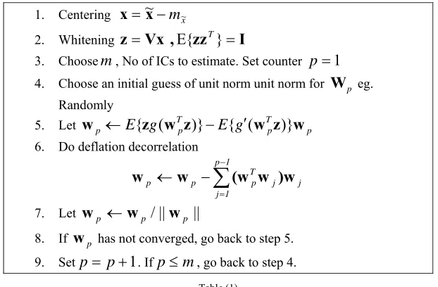
(20)In this section we consider three examples to show the performance of fixed-point ICA based on entropy that use GLF as probability function in which this algorithm show in Tabel (1).
1. Centering
x
~
x
m
~x2. Whitening
z
Vx
,
{
zz
T}
I
3. Choose
m
, No of ICs to estimate. Set counterp
1
4. Choose an initial guess of unit norm unit norm forW
p eg.Randomly
5. Let T p
p T
p
p
E
z
g
w
z
E
g
w
z
w
w
{
(
)}
{
(
)}
6. Do deflation decorrelation
p 11 j
j j T p p
p
w
(w
w
)w
w
7. Let
w
p
w
p/
||
w
p||
8. If
w
p has not converged, go back to step 5. 9. Setp
p
1
. Ifp
m
, go back to step 4.Table (1)
6.1 Example
Consider three speech signals as source in which the mixed matrix
A
and demixing matrixW
are given as follow.
9820
.
4259
.
0214
.
6817
.
2591
.
9527
.
2784
.
8726
.
0125
.
A
and
0158
.
4357
.
1580
.
3657
.
9824
.
7487
.
8745
.
2602
.
8555
.
W
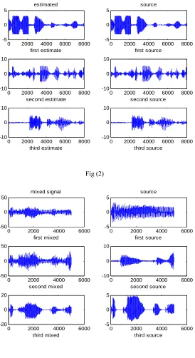
the signals are mixed by (2) ,the mixed signals and sources are show in Fig(1). after using fixed-point ICA algorithm we recover the source as show in Fig(2)
0 2000 4000 6000 8000 -50
0 50
mixed signal
first mixed
0 2000 4000 6000 8000 -20
0 20
second mixed
0 2000 4000 6000 8000 -20
0 20
third mixed
0 2000 4000 6000 8000 -5
0 5
source
first source
0 2000 4000 6000 8000 -10
0 10
second source
0 2000 4000 6000 8000 -10
0 10
third source
6.2 Example
Consider three speech signals as source that mixed with
x
As
in which we considerA
andW
as follow
8220
.
1458
.
2569
.
7817
.
2365
.
8927
.
2684
.
6587
.
4525
.
A
and
1258
.
3253
.
5980
.
7485
.
3545
.
1458
.
4256
.
6902
.
5690
.
W
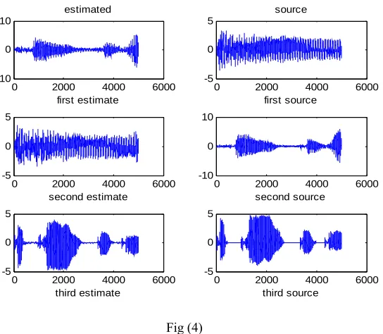
the mixed and source show in Fig (3) .after separation by fixed-point ICA the estimated and source signals show in Fig (4)s
0 2000 4000 6000 8000 -5
0 5
estimated
first estimate
0 2000 4000 6000 8000 -10
0 10
second estimate
0 2000 4000 6000 8000 -10
0 10
third estimate
0 2000 4000 6000 8000 -5
0 5
source
first source
0 2000 4000 6000 8000 -10
0 10
second source
0 2000 4000 6000 8000 -10
0 10
third source
Fig (2)
0 2000 4000 6000 -50
0 50
mixed signal
first mixed
0 2000 4000 6000 -50
0 50
second mixed
0 2000 4000 6000 -20
0 20
third mixed
0 2000 4000 6000 -5
0 5
source
first source
0 2000 4000 6000 -10
0 10
second source
0 2000 4000 6000 -5
0 5
third source
0 2000 4000 6000 -10
0 10
estimated
first estimate
0 2000 4000 6000 -5
0 5
second estimate
0 2000 4000 6000 -5
0 5
third estimate
0 2000 4000 6000 -5
0 5
source
first source
0 2000 4000 6000 -10
0 10
second source
0 2000 4000 6000 -5
0 5
third source
Fig (4)
Performance of GLF
In this section we discuss the performance of using the GLF in which we measure the performance by different ways, first the separation performance for ICA algorithm is evaluated with
the cross-talk error measure
nj n
i l n lj
j i n
i n
j l n il
j i
p
p
p
p
PI
1 1 1 2
2
1 1 1 2
2
1
|
|
max
|
|
1
|
|
max
|
|
(21)
In Table (2) we show the performance of ICA algorithm based on GLF and the function in (8) in which PI of GLF is better than other function and other measure (correlation ,SNR ) show this better.
Method SNR PI correlation
S1 S1 S3 S1_est1 S2_est2 S3_est3
GLF -8.943 -8.943 -8.019 -9.419 -0.9996 -0.9996 0.9981
cosh
log
-6.018 -6.019 -6.0206 -7.940 0.9981 -0.9997 0.9999exp
-2.856 34.708 -2.967 -8.626 0.9968 0.9988 -1.00004
y
-6.016 -6.017 41.122 -8.623 0.9989 0.9991 -0.9999Table (2)
4-Conclusion
In this paper a new non-quadratic function has been proposed for approximation the negentropy which called Generalized Laplace. We estimate the parameters of GLF by two methods ML and kurtosis. The Simulation results show that the negentropy based on GLF is capable of separating signals and the performance of GLF is the best of all other functions that had been proved its performance.
Reference:
[1] Aapo Hyvarinen, Juha Karhunen, Erkki Oja. Independent Component Analysis. John Wiley & Sons (2001).
[3] A.J. Bell, T.J. Sejnowski, An information-maximization approach to blind separation and blind deconvolution, Neural Comput. 7 (6) (1995) 1129–1159.
[4] A.Tesei, C.S.Regazzoni, .Use of fourth-order statistics in non-gaussian noise modeling for signal detection: the Generalized Gausian pdf in terms of kurtosis. In proc. of EUSIPCO-96, sep.1996
[5] B.W. Silverman, Density Estimation for Statistics and Data Analysis, Chapman & Hall, New York, 1986.
[6] B.W. Silverman, Kernel density estimation using the fast Fourier transform, J. Roy. Statist. Soc. Ser. C: Appl. Statist. 31 (1) (1982) 93–99.
[7] D. Erdogmus,J.C. Principe, An error-entropy minimization algorithm for supervised training of nonlinear adaptive systems,IEEE Trans. Signal Process. 50 (7) (2002) 1780–1786.
[8] G. C. Tiao and D. R. Lund, The use of OLUMV estimators in inference robustness studies of the location parameters of a class of symmetric distributions, J. Amer. Statist. Assoc. 65 (1970), 371–386.
[9] M. T. Subbotin, on the law of frequency of errors, Mat. Sb. 31 (1923), 296-300.
[10] R. Boscolo, H. Pan, V. P. Roychowdhury, Non-parametric CA, in: Proceedings of the ICA2001,pp. 13–18.
[11] R. Zeckhauser and M. Thompson, Linear regression with non-normal error terms, The Review of Economics &Statistics 52 (1970), 280–286.
[12] S. Makeig,A.J. Bell, T.-P. Jung,T.J. Sejnowski, Independent component analysis of electroencephalographic data, Adv. Neural Inform. Process. Systems 8 (1996) 145–151.