OPTIMIZATION AND SIZING OF A
GRID-CONNECTED HYBRID PV-WIND
ENERGY SYSTEM
C.S. SUPRIYA*
Saranathan College of Engineering, Venkateswara Nagar,
Panjappur Village, Trichy- 620012
TN, India
M. SIDDARTHAN
Saranathan College of Engineering, Venkateswara Nagar,
Panjappur Village, Trichy- 620012
TN, India
Abstract:
Renewable energy resources such as solar and wind energies are highly advantageous compared to the conventional sources of power in many ways that they clean and available infinitely. But the only drawback is that their outputs depend upon the climatic conditions. Wind-Photovoltaic Hybrid System (WPHS) utilization is becoming popular due to increasing energy costs and decreasing prices of turbines and Photo-Voltaic (PV) panels. However, prior to construction of a renewable generation station, it is necessary to determine the optimum number of PV panels and wind turbines for minimal cost during continuity of generated energy to meet the desired consumption. The aim of this project is to determine the optimal design of a hybrid wind-solar power system for either autonomous or grid-linked applications. The proposed analysis employs quadratic programming techniques to minimize the cost while meeting the load requirements in a reliable manner. Using this procedure, optimum number of PV modules and wind turbines subject to minimum cost can be obtained with good accuracy. Results show that the hybrid systems have considerable reductions in carbon emission and cost of the system.
Keywords: Photo-voltaic, Wind turbines, Hybrid system, Grid-connection, Quadratic Programming, Optimization, Carbon emission
1. Introduction:
Since the oil crisis in the early 1970s, utilization of solar and wind power has became increasingly significant, attractive and cost-effective. In recent years, hybrid PV/wind system (HPWS) has became viable alternatives to meet environmental protection requirement and electricity demands. With the complementary characteristics between solar and wind energy resources for certain locations, hybrid PV/wind system with storage banks presents an unbeatable option for the supply of small electrical loads at remote locations where no utility grid power supply. Since they can offer a high reliability of power supply, their applications and investigations gain more concerns nowadays [13].
context, the present study presents a methodology for the optimal sizing of grid connected PV/wind systems without storage batteries.
Accurate sizing of hybrid PV/wind systems (HPWSs) is of vital importance in renewable energy applications. The aim for sizing is to guarantee the lowest investment with a reasonable and full use of the PV system, wind system, and battery bank at the desired conditions in terms of investment and energy requirement of the specific load. Larger sizing results would cause higher investment whereas smaller sizing may cause load supply discontinuity for a particular load. There are a number of studies about the optimization and sizing of HPWSs. In this study, it is aimed to present a new methodology for HPWS sizing. Therefore, basic energy models are selected and used for keeping the point clear. It can be seen that if more detailed energy models are used for characterizing the system, the idea proposed in this work would still be valid and applicable.
1.1. Hybrid Energy System:
More than 200 million people, live in rural areas without access to grid-connected power. In India, over 80,000 villages remain to be un-electrified and particularly in the state of Tamil Nadu, about 400 villages (with 63% tribes) are difficult to supply electricity due to inherent problems of location and economy [8]. The costs to install and service the distribution lines are considerably high for remote areas. Also there will be a substantial increase in transmission line losses in addition to poor power supply reliability. Like several other developing countries, India is characterized by severe energy deficit. In most of the remote and non-electrified sites, extension of utility grid lines experiences a number of problems such as high capital investment, high lead time, low load factor, poor voltage regulation and frequent power supply interruptions. There is a growing interest in harnessing renewable energy sources since they are naturally available, pollution free and inexhaustible. It is this segment that needs special attention and hence concentrated efforts are continually provided in implementing standalone PV, wind, bio-diesel generator and integrated systems at sites that have a large potential of either solar, wind or both. Traditionally, electrical energy for remote villages has been derived from diesel generators characterized by high reliability, high running costs, moderate efficiency and high maintenance. Hence, a convenient, cost-effective and reliable power supply is an essential factor in the development of any rural area. It is a critical factor in the development of the agro industry and commercial operations, which are projected to be the core of that area’s economy. At present, standalone solar photovoltaic and wind systems have been promoted around the globe on a comparatively larger scale. These independent systems cannot provide continuous source of energy, as they are seasonal. For example, standalone solar photovoltaic energy system cannot provide reliable power during non-sunny days. The standalone wind system cannot satisfy constant load demands due to significant fluctuations in the magnitude of wind speeds from hour to hour throughout the year. Therefore, energy storage systems will be required for each of these systems in order to satisfy the power demands. Usually storage system is expensive and the size has to be reduced to a minimum possible for the renewable energy system to be cost effective. Hybrid power systems can be used to reduce energy storage requirements.
1.1.1. Advantages:
The major advantage of the system is that it meets the basic power requirements of non-electrified remote areas, where grid power has not yet reached. The power generated from both wind and solar components is stored in a battery bank for use whenever required. A hybrid renewable energy system utilises two or more energy production methods, usually solar and wind power.
The main advantage of solar / wind hybrid system is that when solar and wind power production is used together, the reliability of the system is enhanced. Additionally, the size of battery storage can be reduced slightly as there is less reliance on one method of power production. Often, when there is no sun, there is plenty of wind.
Wind speeds are often low in periods (summer, eventually) when the sun resources are at their best. On the other hand, the wind is often stronger in seasons (the winter, in many cases) when there are less sun resources. Even during the same day, in many regions worldwide or in some periods of the year, there are different and opposite patterns in terms of wind and solar resources. And those different patterns can make the hybrid systems the best option in electricity production.
But the hybrid solution is the best option whenever there is a significant improvement in terms of output and performance - which happens when the sun and the wind resources have opposite cycles and intensities during the same day or in some seasons.
1.2. Hybrid System Configurations:
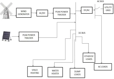
A block diagram of the proposed integrated wind PV generating system is shown in Figure 1.1. This configuration can be used for the study of stand-alone systems as well as network-connected systems. In this case, if the demand is greater than the sum of generation, then power must be supplied by the utility. Furthermore, if the total generated power is greater than the demand, then the excess generation is dumped to an external voltage-controlled resistive load. The purpose of incorporating a dumped load into the system is to preserve the stability of the system frequency and voltage. If the excess energy cannot be dissipated usefully, then it must be disposed as heat by a controlled resistor.
The scope of the project is constrained to certain assumptions. The Peak Power Trackers will keep the wind and PV generators operating at their maximum power operating points. The system is assumed to be connected to the utility throughout and isolated PV panels and/or wind turbines are not taken into consideration. No battery storage or back-up generators are used in the system. The inverter used for DC/AC conversion as shown in Figure 1.1., is assumed to be an ideal one; that is, its efficiency is assumed as cent percent.
1.3. Chapter Organization:
Chapter 1 gives a brief introduction of the proposed project. Chapter 2 deals with the mathematical formulation of the proposed system. Chapters 3 and 4 are two different case studies containing the optimization results for two data. Chapter 5 concludes the project.
2. Mathematical Model of the System:
Modeling the generated energies from wind turbines and PV modules constitutes the critical step for optimization. There are a number of mathematical models in the literature for both PV modules and wind generators. Many of these models consider a variety of physical factors for improving accuracy.
2.1. Basic Mathematical Model of PV Modules:
Output power of PV panels depends on the current produced due to irradiation of solar rays on the module. Thus PS can be written as a function of insolation which is the power produced per unit square metre of the panel. Since we are considering panels of size 1m2, total power is the product of insolation, number of panels and the efficiency of the panel to effectively convert the solar irradiation into electric power. Thus the output power of PV panels [11] can be mathematically expressed as:
where, η and I are energy conversion efficiency, generating power per 1 m2 for 1 MJ/m2, and insolation in kW/m2.
Also the initial and maintenance cost of PV panels per year [11] can be expressed mathematically as follows:
where, Sc is the cost per 1 m2 of PV panel, λs is the reliability coefficient of PV panels, Sy, is the lifetime of PV panels, Sn is the number of PV panels to be determined.
2.2. Basic Mathematical Model of Wind Generator:
Different types of wind generators usually have different power output performance curves. Consequently, the model used to describe their performance should also differ. A typical model for a wind turbine can be considered as:
where, Pw is the output power of wind generator at wind speed V, Pr is the rated power, V is the wind speed at the hub height, and Vci, Vr and Vco are the cut-in, rated and cut-out wind speeds, respectively. Here, n is the number of cubic spline interpolation functions corresponding to n + 1 value couples (speed, power) of data provided by the manufacturers, and a, b, c and d are the polynomial coefficients of the cubic spline interpolation functions, which depend on the wind turbine generator type. Such a model is useful if the power characteristic of wind turbine is available.
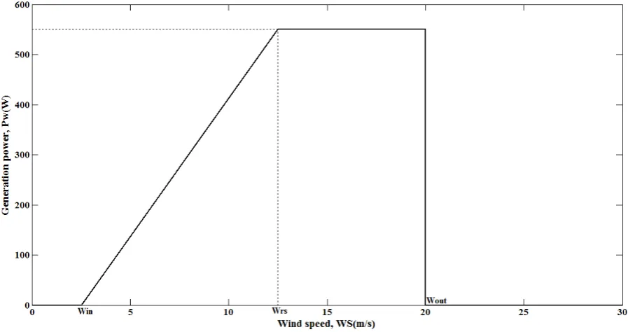
The model we have considered here [11] needs to consider the cut-in wind speed Win and the cut out wind speed Wout. If the wind speed exceeds Win, the wind generator starts generating power, if wind speed exceeds the rated wind speed Wrs, it generates constant power, and if the wind speed exceeds Wout, the wind generator stops running to protect the wind generator as shown in Figure 2.1.
Thus the power output can be mathematically written as follows:
Pw=0 (Wout<WS<Win) (Win<WS<Wrs) Pw=WrpWn (Wrs<WS<Wout)
where, ξ is the slope between Win and Wrs.
n
S I
η
PS = (2.1)
y n c ic
S S S
S =
y n s ic mc
S
S
)
λ
-(1
S
S
=
-3 n in
)
W
x
10
W
ξ(WS-Pw
=
(2.2)
(2.3)
Here, the wind speed is always greater than the cut-in speed and lesser than the rated speed. Thus the wind power output in kW for this case can be written as:
The mathematical model for the cost of wind turbines [11] is also given in terms of the initial and maintenance costs per year as given below:
where, Wc is the cost per one generator of wind turbines, λw is the reliability coefficient of wind turbines, Wy is the lifetime of wind turbines, Wn is the number of wind turbines to be determined.
The wind speed data were taken at a height of four metres. However, the wind turbine hub height was assumed to be 30 metres, thus, the wind data was corrected using the power law expression below [6].
where, Ho = 4 m is the height at which the data are recorded, H = 30 m is the wind turbine hub height, So and S are wind speeds at 4m and 30m respectively. The exponent α is a measure of surface friction and was taken as 0.13 and was confirmed through experimental methods.
2.3. Problem Formulation:
The major concern in the design of an electric power system that utilizes renewable energy sources is the accurate selection of system components that can economically satisfy the load demand. In grid-linked systems, emission is another variable to be minimized for the use of renewable energy be justified [3].
Hence, system's components are found subject to:
minimizing the electricity production cost ($/KWh), ensuring that the load is served reliably, and minimizing the power purchased from the grid.
2.3.1. General Optimization Problem
An optimization or a mathematical programming problem [16] can be stated as follows: -3
n in
)
W
x
10
W
ξ
(WS-Pw
=
y n c ic
W W W W =
y n w ic mc
W W )
λ
-(1 W
W =
(2.5)
(2.6)
α
=
o
H H S
S
o (2.7)
Find
,
.
.
.
X
2 1
=
nx
x
x
which minimizes f (X)
subject to the constraints
, 0 ) (X ≤
gj
j
=
1
,
2
,...,
m
, 0 ) (X =
hj
j
=
1
,
2
,...,
p
where, X is n-dimensional vector called the design vector, f(X) is termed the objective function, and gj(X) and hj(X) are known as inequality or equality constraints respectively. The number of variables n and the number of constraints m and/or p need not be related in any way. The problem stated in equation is called constrained optimization problem.
2.3.2. Objective Function:
The objective function is to minimize the total cost of a grid connected hybrid PV and wind system, Tc. It includes the initial, maintenance and operation costs of the hybrid system [11]. For present work it is assumed that the initial costs are proportional to the number of panels/turbines and the maintenance costs are proportional to their squares.
Min (Tc) = Min (Sic+Smc+Wic+Wmc+CpUp)
where, Sic, Smc are initial and maintenance costs of PV panels, Wic, Wmc are initial and maintenance costs of wind turbines used, Cp is the cost/kWh of power drawn from utility, all in $ and Up is the number of units of electric power to be drawn from the grid.
Therefore, the objective function can be written as:
2.3.3. Constraints:
In our problem, we have not used any inequality constraints. The only condition which has to be satisfied is that the total power generation should always be equal to the load demand. This is given in the form of an equality constraint. Thus, our problem can be summarized as the minimization of the total cost subject to meeting the demand throughout the year by our power generation.
Pdem, indicates the electric energy consumed in an average residence. PV panels, wind turbines supply power for the residence load. If this power cannot satisfy power demand, we buy power from the utility, and if their power is more than power demand, remaining power is dumped.
Thus the constraints are set so as to minimise magnitude of the difference between generated power (Pgen) and the power demand (Pdem).
dem gen
P
P
ΔP
=
−
where,
Pgen = Ps+ Pw+Up
Here, Ps, Pw, Up are the power outputs of solar panels, wind turbines and the power taken from the grid respectively. The total generated and demanded energy (Egen, Edem) over a 24-hour period can be written in terms of the generated wind and solar power and the power demand as follows:
[
]
=Δ
+
Δ
+
Δ
=
8760 1 n p w sgen
(P
)(
T)
(P
)(
T)
(U
)(
T)
E
[
]
= Δ =8760 1 n dem dem (P )( T)E
In order for generation and load to balance over a given period of time, the curve of ∆Pversus time must have an average of zero over the same time period [6] (in this case, over a year). Note that positive values of ∆P indicate the availability of generation and negative ∆Pindicates generation deficiency. An equation of energy versus time (∆E) can be obtained by integrating ∆P.
=
−
=
Δ
Pdt
E
genE
demΔ
E
Hence the constraints can be written as follows:[
]
[
]
= =Δ
=
Δ
+
Δ
+
Δ
8760 1 n 8760 1 nT)
(Pdem)(
T)
(Up)(
T)
(Pw)(
T)
(Ps)(
Since ∆T=1 hour in this case, the constraints can be further modified as:
= = = = + + = 8760 1 n dem 8760 1 n p 8760 1 n w 8760 1 ns P U P
P
Therefore, by substituting the various terms for Ps, Pw, the constraints can be written as:
= = = − ==
+
×
−
+
8760 1 n dem 8760 1 n 8760 1 n p 3 n in 8760 1 nn
ξ(WS
W
)
W
10
U
P
ηIS
Thus, the objective function of the above formulation is a quadratic function of the decision variables, that is, the number of panels, number of turbines and the number of units of electrical power to be purchased from the utility. And the constraint is a linear equation in terms of the same decision variables. This makes it clear that quadratic programming can be used to solve this problem.
2.4. Implementation of Quadratic Programming for the Above Problem:
Objective function =
Obj. Fn. =
subject to:
= = = − =
=
+
×
−
+
8760 1 n dem 8760 1 n 8760 1 n p 3 n in 8760 1 nn
ξ(WS
W
)
W
10
U
P
ηIS
+
−
+
+
−
+
p py n w c y n c y n s c y n c
U
C
W
W
)
λ
(1
W
W
W
W
S
S
)
λ
(1
S
S
S
S
min
2 2 2 2[
]
+ − − p n n p y c y c p n n y w c y s c p n n U W S C W W S S U W S 0 0 0 0 W ) λ (1 W 0 0 0 S ) λ (1 S U W S min 2 2[
]
[
dem]
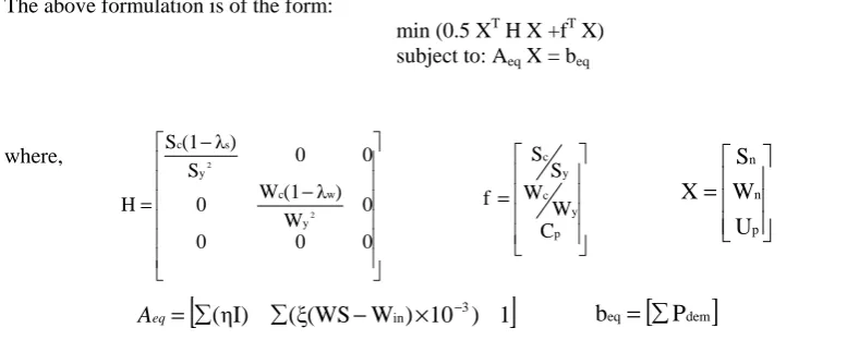
The above formulation is of the form:
min (0.5 XT H X +fT X) subject to: Aeq X = beq
where,
Thus, quadratic programming is used to solve the above optimization problem.
2.5. List of Data used for the Mathematical Model
3. Case Study 1:
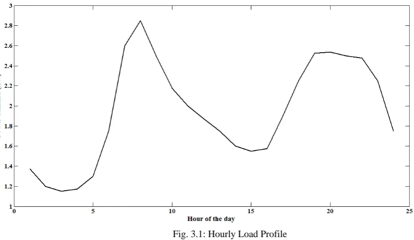
The optimization procedure discussed above has been used for component sizing for a stand-alone hybrid (wind/PV) system to supply the electrical power needs of a house on a ranch assumed to be located at a sight in a remote area in South-Central Montana [6]. As it is located in a remote area, the cost of buying power from the grid is costlier when compared to other areas. The annual average hourly load profile for the house is shown in Figure 3.1. It is a good representation of the electrical demand of a typical residential home in the Pacific Northwest. Note that the curve of load demand, being an average hourly demand curve, is shown as a continuous plot. Therefore, the wind, insolation and energy curves are also shown as continuous plots. If the hourly demand data is assumed to be discontinuous (constant during each hour), then all of the curves will be stair case plots.
− − = 0 0 0 0 W ) λ (1 W 0 0 0 S ) λ (1 S H 2 2 y w c y s c = p n n U W S X
[
(ηI) (ξ(WS−Win)×10−3) 1]
=
eq
A beq=
[
Pdem]
= p y c y c C W W S S f (2.21) Photovoltaic (US-64)
Output power per 1MJ/m2 130W/m2 Conversion efficiency 16% Initial cost per 1m2 $780 Reliability Co-efficient 0.95
Life time 25 years
Wind turbine (AIR 403 Land)
Maximum output power 550W
Cut-in speed 2.5m/s
Cut-out speed 20m/s
Rated speed 12.5m/s
Initial cost $1440
Reliability Co-efficient 0.90
Life time 13 years
Grid
The Figure 3.2 shows the hourly average wind speed data over two years recorded by a data acquisition system installed at the site where the house is assumed to be located.
A pyranometer was also installed at the site, for recording insolation data. An hourly average curve of insolation (over one year) obtained from the measured data is shown inFigure 3.3.
Fig. 3.1: Hourly Load Profile
3.1. Study of Different Configurations:
The data above are considered to be inputs for the hybrid system and the optimization is run as per the suggested mathematical model, using quadratic programming. By interconnecting and/or disconnecting different components such as the PV panels and wind turbines, four configurations are formed, the results of which are tabulated and compared at the end.
A. Conventional grid system B. Grid connected PV system C. Grid connected wind system D. Grid connected hybrid system
The figures obtained by optimization for all four cases are shown under each case. The results are tabulated in tables under each case. In the following outputs, the maximum number of turbines and panels are fixed arbitrarily.
3.1.1. Conventional Grid System
Fig 3.3: Solar Insolation Data
The Figure 3.4 shows the graph, in which the load is met only by the power from the grid. As we have considered a remote area, the per unit cost of the utility is itself very costly. So the total cost of this system becomes very high and carbon emission is high too.
3.1.2. Grid Connected PV System
Now, the wind turbines are disconnected from the system and the whole load demand is assumed to be satisfied by a number of PV panels (32 in this case). The deficit in power is supplied by the utility. The shaded region in Figure 3.5 shows the excess generation at certain parts of the day.
The excess generation is very meagre in this case, as the solar insolation is high only at certain parts of the day. Also there is no generation during the night times. Due to these reasons, the power drawn from the utility is more in this case, proportionally CO2 emission increases. The high cost of PV panels also makes this system much costlier.
So generating power from PV panels alone when sufficient wind speed is also available, is not a very good option.
3.1.3. Grid Connected Wind System
In this case, the PV panels are removed from the system and 4 wind turbines are assumed to suffice the load demand. The excess demand is met by the power from utility. The Figure 3.6 shows the graph obtained for wind only system.
From the data we have considered, it is seen that the wind speed in the area is much higher than the cut-in speed. So the generation is high throughout the day. This reduces the amount of power drawn from the grid and thereby the CO2 emission. When the cost is considered, it is seen that the cost of wind-only system is lower when compared to hybrid system. So this system is considered to be a better option when compared to the others.
3.1.4. Grid Connected Hybrid System
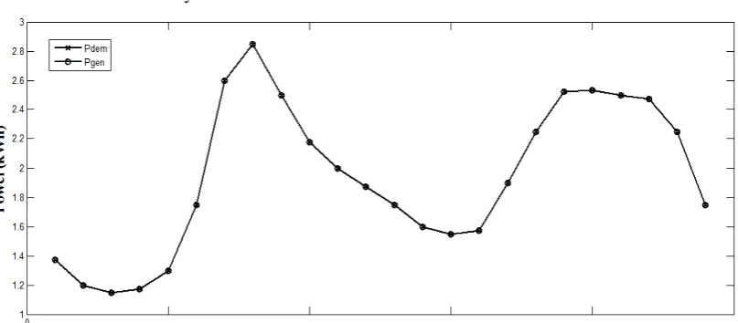
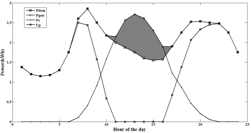
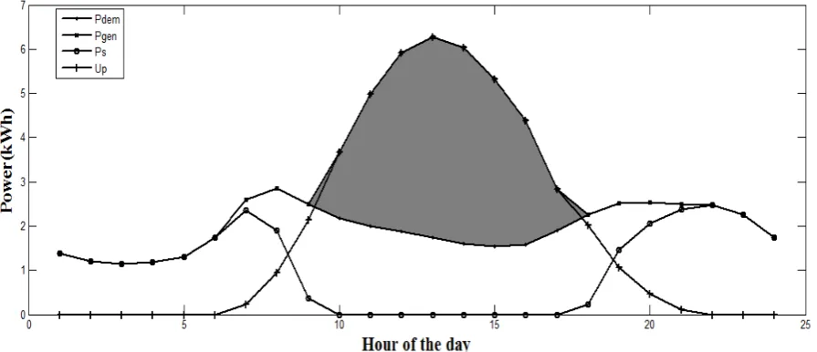
In this case both solar panels and wind turbines are connected to the grid and Figure 3.7 is obtained. 8 panels and 4 turbines are being used. It shows power demand (Pdem) Vs power generated (Pgen). The power generated (Pgen), is the sum of power generated from solar (Ps), wind (Pw) and the power drawn from the utility (Up) respectively.
From the Figure 3.7 we see that, the demand and total generation are same mostly. The shaded regions in the Figure 3.7 represent the area where the power generation exceeds the demand. This is obtained especially at noon when both solar radiation and wind speeds are high. This excess power is dumped through external resistance.
It can be seen that the demand is mostly satisfied by the PV panels and wind turbines, and the power drawn from the grid is minimum. Thus there will be a considerable reduction in the amount of CO2 emitted from the system. The cost also works out to be economical, which proves that renewable energy sources are used at a much lower rate to supply power, especially in remote areas, such as the one considered here.
3.2. Fixing the Maximum Number of Panels and Turbines:
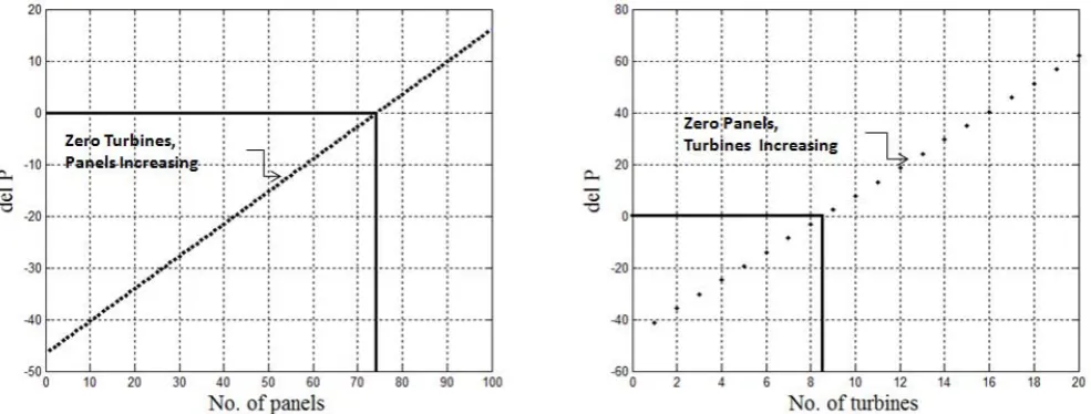
These results do not have any proper basis for the fixing of upper limits of PV panels and wind turbines. The maximum number of panels and turbines for a grid connected PV system and a grid connected wind system respectively can be found out by plotting ∆P against number of panels and number of turbines and the point where the curve coincides with the X-axis is taken as the maximum number.
From Figure 3.8, the maximum number of panels and turbines can be rounded off to 74 and 8 respectively. Now, using these results, optimization is run.
3.3. Optimization Results:
The results obtained by fixing the maximum number of panels and turbines are shown in the following figures and the final result is tabulated
Fig 3.7: Load Demand and Generation of a Grid Connected Hybrid System
3.3.1. Conventional Grid System
There is no change in the conventional system due to optimization. It is exactly the same as Figure 3.4.
3.3.2. Grid Connected PV System
Optimization results for this configuration generate the Figure 3.10, where the generation far exceeds the demand during noon hours, but power is completely drawn from grid during night times. Cost is very high for this configuration. Table 3.5 contains the optimized results.
3.3.3. Grid Connected Wind System
The Figure 3.10 is quite similar to the one obtained in Figure 3.6. The cost is lowest for this system and only a small amount of CO2 is emitted. Table 3.6 shows the results for the optimized case.
Fig 3.9: Load Demand and Generation of a Grid Connected PV System for Optimized Number of Panels and Turbines
3.3.4. Grid Connected Hybrid System
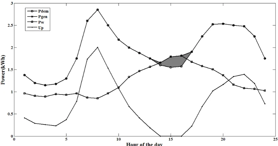
The Figure 3.11 has the same trend as the one obtained for this system as in Figure 3.7 except that the number of turbines used has been increased and panels decreased, owing to the economics of wind power compared to solar. The cost and carbon emission are also quite less for this case. Table 3.7 contains the results for optimum panels and turbines.
3.4. Comparison of Results:
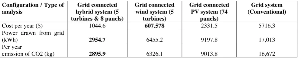
The Table 3.1 compares the results of the above four cases in terms of cost and power drawn from the grid. It is found that 0.98kg of CO2 is emitted from one unit of electric power produced by the utility [15]. Thus the comparison in the amount of carbon given to the atmosphere in each case is also tabulated in Table 3.1. The best system based on each criterion is highlighted.
Configuration / Type of analysis
Grid connected hybrid system (5 turbines & 8 panels)
Grid connected wind system (5
turbines)
Grid connected PV system (74
panels)
Grid system (Conventional)
Cost per year ($) 1044.6 607.578 2331.5 5716.3
Power drawn from grid
(kWh) 2954.7 6455.2 9197.8 17,013
Per year
emission of CO2 (kg) 2895.9 6326.1 9013.8 16,672
From the Table 3.1, it is clear that the grid-hybrid system is better than all the other configurations for reducing the amount of emitted CO2. Cost comparison also shows only a small differential than the grid-wind system.
3.5. Cost and Carbon Emission for Increasing Number of Panels and Turbines:
The overall cost of the system, which is our objective function, is found to be linearly increasing with increase in number of panels and/or turbines.
Another important advantage in using the renewable energy systems instead of buying power from the utility is that it reduces the amount of carbon emission, thus reducing the effect of global warming.
Fig 3.11: Load Demand and Generation of a Grid Connected Hybrid System for Optimized Number of Panels and Turbines
Thus, by increasing the number of panels and/or turbines, the amount of CO2 emitted by the system as a whole would be considerably reduced. The plot between the system cost and carbon emission is found to be an exponentially decreasing curve.
Our objective not only lies in minimising the system cost, but also in reducing the carbon emission by increasing the use of renewable energy sources
3.6. Optimized Region for Hybrid Configuration:
Now for finding out the optimum result of the grid connected hybrid system, the cost versus carbon emission curves for PV-grid and wind-grid systems are plotted together. The hybrid system cost obtained for the optimal configuration is projected and a closed region for searching the appropriate number of panels and turbines is shown in Figure 3.12.
If a restriction is given on the amount of carbon emission as per law, it can be projected and the exact number of PV panels and wind turbines can be obtained as the optimal configuration.
4. Case Study II:
The proposed optimization scheme is tested for another yearly data which gives the hourly average data for load profile, wind speed and solar insolation all through the year. The annual demand for this profile is approximately 39MW. A part of this data showing the load demand, wind speed and solar insolation for the month of January is shown in figures 4.1, 4.2 and 4.3.
0 100 200 300 400 500 600 700 800 0
2 4 6 8 10 12 14
Hour of the month January
L
o
a
d
d
e
m
a
n
d
(kWh)
0 100 200 300 400 500 600 700 800
2 4 6 8 10 12 14 16
Hour of the month January
W
in
d
sp
e
e
d
(m
/s)
Fig.4.1: Hourly Load Profile for January
Similar studies are done for this data also and the results and graphs are shown.
4.1. Study of Different Configurations:
The same configurations which were considered for case 1 are considered here too and optimization is run first by fixing the number of turbines and panels arbitrarily.
4.1.1. Conventional Grid System
The Figure 4.4 shows the graph, in which the load is met only by the power from the grid. As we have considered a remote area, the per unit cost of the utility is itself very costly. So the total cost of this system becomes very high. Table 4.1 shows the results.
0 100 200 300 400 500 600 700 800
0 0.2 0.4 0.6 0.8 1 1.2 1.4
Hour of the month January
In
so
la
tio
n(kW
/m2
)
4.1.2. Grid Connected PV System
Now, the wind turbines are disconnected from the system and the whole load demand is assumed to be satisfied by a number of PV panels. The deficit in power is supplied by the utility. Figure 4.5 shows the generation and demand for this configuration.
It is vivid from the Figure 4.6 that the solar power generated is very less and more power is drawn from the grid. This proportionally increases CO2 emission. Also the system cost is high due to high cost of panels. So this configuration has no specific advantages.
4.1.3. Grid Connected Wind System
In this case, the PV panels are removed from the system and wind turbines are assumed to suffice the load demand. The excess demand is met by the power from utility. The excess power generated is shown in shaded areas. Figure 4.7 shows graph plotted between demand and generation.
Fig 4.5: Load Demand and Generation of a Grid Connected PV System
From Figure 4.7, we see that the generation exceeds demand in few hours of the day. Since the power drawn is reduced during those hours, the CO2 emission is also reduced. The split up of power generation vs the load demand is shown in Figure 4.8.
4.1.4. Grid Connected Hybrid System
In this case both solar panels and wind turbines are connected to the grid and the following graphs are obtained. Figure 4.9 shows power demand (Pdem) vs power generated (Pgen). The power generated (Pgen), is the sum of power generated from solar (Ps), wind (Pw) and the power drawn from the utility (Up) respectively.
Fig 4.7: Load Demand and Generation of a Grid Connected Wind System
The shaded region shows the region where the generation of power exceeds the load demand. The excess power obtained is dumped through external resistance.
Figure 4.10 shows the split up of power generation along with the load demand. The split up includes generation of power by solar, wind and power drawn from utility.
From the Figure 4.10, we see that the use of hybrid system reduces the amount of power drawn from the grid, thus the amount of CO2 emitted from the grid is reduced, thus reducing the global warming. Also the cost of producing energy is reduced.
4.2. Fixing the Maximum Number of Panels and Turbines:
These results do not have any proper basis for the fixing of upper limits of PV panels and wind turbines. The maximum number of panels and turbines for a grid connected PV system and a grid connected wind system
Fig 4.9: Load Demand and Generation of a Grid aConnected Hybrid System
respectively can be found out by plotting P against number of panels and number of turbines and the point where the curve coincides with the X-axis is taken as the maximum number.
From Figure 4.11, the maximum number of panels and turbines can be rounded off to 135 and 13 respectively. Now, using these results, optimization is run.
4.3. Optimization Results:
The results obtained by fixing the maximum number of panels and turbines are shown in the following graphs and the final results are tabulated.
4.3.1. Conventional Grid System
The plot is same as the one obtained in Figure 4.4. The cost is highest for this system and carbon emission is very high.
4.3.2. Grid connected PV system
Optimization results for this configuration generate the graphs Figure 4.12 and Figure 4.13 where the generation never exceeds the demand throughout the day. Thus power is drawn from the grid continuously. Cost is very high for this configuration, so is carbon emission. Table 4.5 shows the results.
4.3.3. Grid Connected Wind System
Figures 4.14 and 4.15 are quite similar to the ones obtained previously. The cost is lowest for this system and only a small amount of CO2 is emitted. They show the optimization results and the split-up for the power generations.
Fig 4.12: Load Demand and Generation of a Grid Connected PV System for Optimized Number of Panels and Turbines
4.3.4. Grid Connected Hybrid System
Now optimization is run for grid connected hybrid system with fixed number of panels and turbines. Figure 4.16 follows the same trend, but numbers of turbines are increased as increasing the panels would make the cost very high.
From Figure 4.16, we can clearly see that generation increases demand in many parts of the day. This indicates that power drawn from grid is very less. This would reduce the amount of carbon emission. The Figure 4.17 shows the split up of power generation along with the load demand.
Fig 4.14: Load Demand and Generation of a Grid Connected Wind System for Optimized Number of Panels and Turbines
4.4. Comparison of Results:
The Table 4.1 compares the results of the above four cases in terms of cost and power drawn from the grid. It is found that 0.98kg of CO2 is emitted from one unit of electric power produced by the utility [15]. Thus the comparison in the amount of carbon given to the atmosphere in each case is also tabulated in Table 4.1. The best system based on each criterion is highlighted.
Fig 4.16: Load Demand and Generation of a Grid connected Hybrid System for Optimized Number of Panels and Turbines
Configuration / Type of analysis
Grid connected hybrid system (13 turbines & 8 panels)
Grid connected wind system (13
turbines)
Grid connected PV system (135
panels)
Grid system (Conventional)
Cost per year ($) 1690 1440.4 4213 13098
Power drawn from grid
(kWh) 9922.2 10597 22054 38982
Per year
emission of CO2 (kg) 9723.8 10597 21612 38202
From the Table 4.1, it is clear that the grid-hybrid system is better than all the other configurations for reducing the amount of emitted CO2. Cost comparison also shows only a small differential than the grid-wind system.
4.5. Cost and Carbon Emission for Increasing Number of Panels and Turbines:
The overall cost of the system, which is our objective function, is found to be linearly increasing with increase in number of panels and/or turbines.
Another important advantage in using the renewable energy systems instead of buying power from the utility is that it reduces the amount of carbon emission, thus reducing the effect of global warming.
Thus, by increasing the number of panels and/or turbines, the amount of CO2 emitted by the system as a whole would be considerably reduced. The plot between the system cost and carbon emission is found to be an exponentially decreasing curve and is shown below.
Our objective not only lies in minimising the system cost, but also in reducing the carbon emission by increasing the use of renewable energy sources.
4.6. Optimized Region for Hybrid Configuration:
Now for finding out the optimum result of the grid connected hybrid system, the cost versus carbon emission curves for PV-grid and wind-grid systems are plotted together. The hybrid system cost obtained for the optimal configuration is projected and a closed region for searching the appropriate number of panels and turbines is shown in Figure 4.18.
If a restriction is given on the amount of carbon emission as per law, it can be projected and the exact number of PV panels and wind turbines can be obtained as the optimal configuration.
To conclude, the grid connected wind systems happens to be the best configuration in both the cases on considering cost. But if we can spend a little more, considering PV panels also is not a bad option, in a way that it further decreases the amount of power drawn from the grid and hence the carbon emission and global warming.
This project proves that using renewable sources is far better than the conventional grid system especially in remote areas where the per unit cost of utility is itself very high. The proposed system reduces both the cost and the amount of CO2 emitted from the entire setup.
5.1. Future Scope:
• Now-a-days more energy efficient solar panels are coming into commercial market. If the efficiency can be increased further, there will be a proportionate decrease in the cost as one module of PV array would be able to produce more power at a lower cost. This would make the grid-PV system and the grid-hybrid system more economical.
• A selling price could be incorporated by signing a contract with the electricity board that we could sell the excess power produced instead of dumping it. If this could be brought into use, the hybrid system would become more economical than the grid-wind system itself as the excess generation won’t be wasted. There is a probability that sometimes we may earn more than we spend, if solar insolation and wind speeds are high during a particular year. Hence the grid-hybrid system would become the best configuration in future in terms of both cost and carbon emission.
Acknowledgement:
We take immense pleasure in expressing our thanks to the Secretary Sri. S. Ravindran, Principal Dr. Y. Venkatramani, Director (Administrative) Prof. V. Nagarajan for providing us a good ambience to conduct out project successfully.
We will fail in our duty if we do not express our heart-felt thanks to our Head of the Department Dr. M. Arutchelvi, for her constant source of inspiration and motivation towards the completion of our project.
“A good teacher is worth million books”. We feel relish in thanking our guide Dr. M. Varadarajan for his encouragement and support during the project work. We appreciate the involvement and interest he showed throughout the period, guiding us perfectly and giving his valuable suggestions.
Also we take this opportunity to thank our entire department staff. We want to thank our non-teaching staff as well for their support in the laboratory.
We specially thank our parents for their moral support and encouragement in carrying out this project.
Finally, we thank all our friends who motivated us and made this project a grand success.
References:
[1] Ashok, S., “Optimised Model for Community-Based Hybrid Energy System” RENEWABLE ENERGY,VOL.32,NO.7,JUNE 2007,PP: 1155–1164.
[2] Bagul, A.D., Salameh, Z.M., Borowy, B., “Sizing of Stand-Alone Hybrid PV/Wind System using a Three-Event Probabilistic Density Approximation.” JOURNAL OF SOLAR ENERGY ENGINEERING,VOL.56,NO.4,1996,PP:323-335.
[3] Chedid, R., and Rahman, S., “Unit Sizing and Control of Hybrid Wind-Solar Power Systems” IEEETRANSACTIONS ON ENERGY
CONVERSION,VOL.12,NO.1,MARCH 1997,PP:79-85.
[4] Chedid, R., Saliba, Y., “Optimization and Control of Autonomous Renewable Energy Systems” INTERNATIONAL JOURNAL ON
ENERGY RESEARCH,VOL.20,NO.7,1996,PP:609-624.
[5] Karaki, S.H., Chedid, R.B., Ramadan, R., “Probabilistic Performance Assessment of Autonomous Solar-Wind Energy Conversion Systems.” IEEETRANSACTIONS ON ENERGY CONVERSION,VOL.14,NO.3,SEPTEMBER 1999,PP:766-772.
[6] Kellogg, W.D., Nehrir, M.H., Venkataramanan, G. and Gerez, V., “Generation Unit Sizing and Cost Analysis for Stand-Alone Wind, Photovoltaic and Hybrid Wind/PV Systems” IEEETRANSACTIONS ON ENERGY CONVERSION,VOL.13,NO.1,MARCH 1998,PP: 70-75.
[7] Kellogg, W.D., Nehrir, M.H., Venkataramanan, G. and Gerez, V., “Optimal Unit Sizing for a Hybrid PV/Wind Generating System.” ELECTRIC POWER SYSTEM RESEARCH,VOL.39,1996,PP:35-38.
[8] Muralikrishna, M., Lakshminarayana, V., “Hybrid (Solar and Wind) Energy Systems for Rural Electrification” ARPNJOURNAL OF ENGINEERING AND APPLIED SCIENCES,VOL.3,NO.5,OCTOBER 2008,PP:50-58
[9] Musgrove, A.R.D., “The Optimization of Hybrid Energy Conversion System using the Dynamic Programming Model – RAPSODY.” INTERNATIONAL JOURNAL ON ENERGY RESEARCH,VOL.12,1988,PP:447-457.
Using Genetic Algorithm” IEEETRANSACTIONS ON ENERGY CONVERSION,VOL.21,NO.2,JUNE 2006,PP:459-466.
[12] Wang, C., Nehrir, M.H., “Power Management of a Stand-Alone Wind/Photovoltaic/Fuel Cell Energy System” IEEETRANSACTIONS ON ENERGY CONVERSION,VOL.23,NO.3,SEPTEMBER 2008,PP:957-967.
[13] Yang, H.X., Burnett, J., Lu, L., “Weather Data and Probability Analysis of Hybrid Photovoltaic Wind Power Generation Systems in Hong Kong.” RENEWABLE ENERGY,VOL.28,2003,PP:1813-1824.
[14] Yokoyama, R., Ito, K., Yuasa, Y., “Multi-Objective Optimal Unit Sizing of Hybrid Power Generation Systems Utilizing PV and Wind Energy.” JOURNAL OF SOLAR ENERGY ENGINEERING,VOL.116,1994,PP:167-173.
[15] Energy Analysis of Power Systems - World Nuclear Association [Online], 2009[Cited July 2009]; Available from: http://www.world-nuclear.org/info/inf11.html