Generating prior probabilities for classifiers of brain tumours using belief networks

Open Access

Research article

Generating prior probabilities for classifiers of brain tumours using

belief networks

Greg M Reynolds

_{, Andrew C Peet*}

_{and Theodoros N Arvanitis}

Address: 1_{Department of Electrical, Electronic and Computer Engineering, University of Birmingham, Birmingham, UK and} 2_Academic

Department of Paediatrics and Child Health, University of Birmingham, UK and Birmingham Children's Hospital NHS Foundation Trust, Birmingham, UK

Email: Greg M Reynolds - [email protected]; Andrew C Peet* - [email protected]; Theodoros N Arvanitis - [email protected] * Corresponding author

Abstract

Background: Numerous methods for classifying brain tumours based on magnetic resonance spectra and imaging have been presented in the last 15 years. Generally, these methods use supervised machine learning to develop a classifier from a database of cases for which the diagnosis is already known. However, little has been published on developing classifiers based on mixed modalities, e.g. combining imaging information with spectroscopy. In this work a method of generating probabilities of tumour class from anatomical location is presented.

Methods: The method of "belief networks" is introduced as a means of generating probabilities that a tumour is any given type. The belief networks are constructed using a database of paediatric tumour cases consisting of data collected over five decades; the problems associated with using this data are discussed. To verify the usefulness of the networks, an application of the method is presented in which prior probabilities were generated and combined with a classification of tumours based solely on MRS data.

Results: Belief networks were constructed from a database of over 1300 cases. These can be used to generate a probability that a tumour is any given type. Networks are presented for astrocytoma grades I and II, astrocytoma grades III and IV, ependymoma, pineoblastoma, primitive neuroectodermal tumour (PNET), germinoma, medulloblastoma, craniopharyngioma and a group representing rare tumours, "other". Using the network to generate prior probabilities for classification improves the accuracy when compared with generating prior probabilities based on class prevalence.

Conclusion: Bayesian belief networks are a simple way of using discrete clinical information to generate probabilities usable in classification. The belief network method can be robust to incomplete datasets. Inclusion of a priori knowledge is an effective way of improving classification of brain tumours by non-invasive methods.

Background

The current "gold standard" for brain tumour diagnosis is histopathology which requires a sample of tumour

obtained at operation. These operations have an inherent risk of morbidity and mortality. Magnetic Resonance Imaging (MRI), Magnetic Resonance Spectroscopy (MRS)

Published: 18 September 2007

BMC Medical Informatics and Decision Making 2007, 7:27 doi:10.1186/1472-6947-7-27

Received: 12 May 2007 Accepted: 18 September 2007

This article is available from: http://www.biomedcentral.com/1472-6947/7/27

© 2007 Reynolds et al; licensee BioMed Central Ltd.

and other imaging modalities may offer a non-invasive way of making a diagnosis, but no method has yet attained sufficient accuracy to replace histopathology. MRS in particular has been shown to provide useful infor-mation about the biochemical content of a brain tumours [1] and numerous methods for classifying brain tumours based on magnetic resonance spectra have been presented [2-6].

When making a classification decision it is intuitively sen-sible to use as much relevant information as possen-sible, but very few of the published classifiers have attempted to combine information from different modalities and sources (but see [7-10]). This work details a method which uses data from the West Midlands Regional Child-hood Tumour Registry (WMRCTR) to produce probabili-ties of brain tumour class, given its anatomical location.

The WMRCTR provides data from the last five decades on over 1700 childhood cancer patients, mostly in free-text form. During that period the format of the stored data has changed: knowledge of the exact anatomical location has improved with the advent of MRI and the classification scheme for tumours has changed to the WHO [11] sys-tem. This presents a considerable challenge to its use in computer-based systems.

The discriminating power of "anatomical location" as a feature for a classifier is not sufficient to make classifica-tions based on this variable alone. However it is envisaged that the probabilities obtained from the WMRCTR data could be used as "informative priors" in existing classifica-tion methods. In this work we demonstrate their impact on a simple MRS based classifier. It is worth emphasising that this work focusses on paediatric brain tumours, which are significantly more varied and more difficult to diagnose using MRI alone, than those in adults.

The approach to using the WMRCTR data is based on a graphical representation of Bayesian inference called belief networks. Since anatomical location and tumour class are discrete random variables, probabilities can be estimated directly from the data, without the need to rely on assumptions about the form of probability density func-tions. In the following sections we introduce the belief network method, present some examples and discuss the construction of the final network from the data in the WMRCTR. Finally, the network is presented and demon-strated on some test-cases.

Methods

Belief networks

A Bayesian belief network or often just belief network is a graphical representation of the joint probability distribu-tion funcdistribu-tion of a collecdistribu-tion of variables [12,13]. A belief

network makes exactly the same inferences as would be made by applying Bayes' rule to a series of probabilities, but the graphical construction often provides insight into the problem. The network is represented as a weighted, acyclic, directed graph, each vertex representing a discrete variable/event (see Figure 1). To use the terminology of Russell and Norvig [12], each of these vertices fall into one of three categories:

1. query variables, i.e. events the probability of which is of interest (in Figure 1 these are "medulloblastoma" and "astrocytoma");

2. evidence variables, i.e. events known to have occurred (in Figure 1 these are taken to be "posterior fossa" and "supratentorial");

3. hidden variables, i.e. events which may occur but cannot be measured (in Figure 1 these are taken to be "IV ventri-cle" and "cerebellum").

The weighted edges connecting vertices represent the probability that the target vertex is true, conditioned on the source vertex. Here, vertices represent anatomical loca-tions or tumour types. If an edge connects two anatomical locations then its weight is the probability that the tumour was in the target vertex, given that it is known to be in the source vertex. If an edge connects an anatomical location to a tumour type then its weight is the probability that the tumour is of the type specified by the target vertex, given that it is known to have occurred in the source ver-tex.

A simplified belief network showing conditioned probabilities of events

Figure 1

A simplified belief network showing conditioned probabilities of events. The vertex numbers are shown in brackets, refer to the adjacency matrix representation in (1). The numbers shown are purely for pedagogical purposes, for the correct and complete graph refer to Table 1 and Figure 2.

posterior fossa (v1)

supratentorial (v2)

cerebellum (v4) IV ventricle

(v3)

medulloblastoma (v5)

astrocytoma (v6)

2

7 57

2 2 25

To illustrate the utility of the method, consider the follow-ing example. Referrfollow-ing to Figure 1, suppose it is known that the tumour occurs in the posterior fossa (vertex v₁) and the probability that the tumour is a medulloblastoma is sought. Working backward from vertex v₅ (the medul-loblastoma) and applying Bayes' rule:

Of course, if it was known that the tumour occurred in the IV ventricle then the expression could have stopped there and the probability obtained by inspection, thus hidden variables may sometimes be evidence variables depending on the particular sample. The important point is that dif-ferent "resolution" information can be used, this is partic-ularly important if a tumour spans several regions, as will be discussed later. It also means that data of lower resolu-tion can be incorporated into the network. For example, many tumours in the WMRCTR are just listed as having location: "posterior fossa". Working back from the query variables is relatively complicated to implement. An easier and equivalent way is to work forward from the evidence variables. As such it is convenient to represent a graph as an adjacency matrix, for the example in Figure 1 this is:

Each element a_ij of A refers to the weighted connection from vertex v_i to v_j, i.e. the row index refers to the source vertex, the column index to the target.

The adjacency matrix representation permits easy calcula-tion of the vector of class probabilities, given knowledge of which evidence variables to use. To find the probabili-ties of each class, given any evidence variable the follow-ing procedure is used (more computationally efficient methods are given in [12]):

1. Construct the n-dimensional column vector x where n

is the number of vertices (variables) and set all the ele-ments to zero.

2. Set the single element of x that corresponds to the evi-dence variable known be to true, to one.

3. Compute x ←AT_{x until x stops changing. At every} iter-ation, those vertices connected to those with non-zero entries x will become non-zero.

4. Those elements of x corresponding to output variables have the probability that the tumour belongs to each class, given the evidence. All other elements of x will be zero.

Clearly, the axioms of probability require that the sum of all elements in x is unity. It is important to note that the terminating vertices (v₅ and v₆ in Figure 1) need to be con-nected to themselves so that the method just described will converge to the correct value. If they are not present, x will converge to the zero vector. As well as giving proba-bilities of class membership given a single location, tumours that span adjacent anatomical regions can also be considered; for every region in which the tumour is present compute the output vector, then average these to produce the final vector of probabilities. Although this is an intuitively sensible property, it has not been evaluated in this work.

Data processing

The WMRCTR database was made available as a spread-sheet giving hand-typed strings for the diagnosis and loca-tion of each case. Occasionally, grade of tumour was also specified. In total there were 1712 cases available. By hand, each record was examined and modified. If the tumour type was classified with the WHO system, it was left unchanged. If a WHO equivalent existed for a tumour classified using the old scheme, then it was changed; oth-erwise the record was removed. This reduced the number of cases to 1367. These cases were then further reviewed, and only those tumours with location specified were included, reducing the final number of cases used to 1333. Of these, the site of the primary lesion was often only specified vaguely, e.g. "posterior fossa" or "cere-brum". Tumours specified with a greater degree of accu-racy were then grouped (by hand) under these broader headings, as well as maintaining their original informa-tion. A graph showing the anatomical distinctions made is given in Figure 2. Very occasionally, the location was spec-ified in great detail (e.g. "foramen of Munro") but this was very rare and these samples were marked as being in the appropriate containing location.

P

P

( )

( medulloblastoma|posterior fossa

medulloblastoma|IV ve

=

n ntricle IV ventricle|posterior fossa medulloblastom

)

( )

(

× +

P

P aa|cerebellum

cerebellum|posterior fossa )

( )

× =

× + × =

P

2 2

2 7

2 5

5 7

4 7 7

A=



            

0 0 2

7 5

7 0 0

0 0 0 0 0 8

8

0 0 0 0 2

2 0

0 0 0 0 2

5 3 5

0 0 0 0 1 0

0 0 0 0 0 1





            

The classes used were: astrocytoma grades I and II, astro-cytoma grades III and IV, ependymoma, pineoblastoma, PNET, germinoma, medulloblastoma, craniopharyngi-oma and a group representing rare tumours, "other" (classes represented by fewer than 15 cases). It is common practice to group paediatric astrocytomas of different grades in this way as they thought to be very similar dis-eases.

Results and discussion

The simplest method to represent the results would be an adjacency matrix, but this is too large for publication in its direct format. Instead, the graph is specified by Table 1; an

adjacency list representation. A subgraph of the final belief network is shown in Figure 2, giving the paths necessary to generate a probability for a medulloblastoma.

Figure 2 indicates that medulloblastomas have been recorded in the database as occurring in several locations in the brain. Typically however, they are thought to arise from the cerebellum. The IV ventricle and the brain stem are adjacent to the cerebellum and are often invaded by these tumours making it impossible to be certain of the location from which the tumour originated. This illus-trates the power of the belief network in dealing with this situation; the possibility of the tumour being a medullob-lastoma is not discounted if it does not occur in the typical position.

Figure 2 also illustrates another feature of the network arising from the fact that a large amount of historical data was used: a small number of medulloblastomas were also recorded as being present in the parietal and temporal

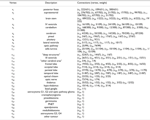
Table 1: Adjacency list representation of final belief network. The destination vertices from each vertex are shown in the "Connections" column

Vertex Description Connections (vertex, weight)

v₁ posterior fossa (v₃, 222/631), (v₄, 109/631), (v₅, 300/631)

v2 supratentorial (v6, 276/702), (v7, 67/702), (v8, 21/702), (v9, 17/702), (v10, 99/702), (v11,

104/702), (v12, 67/702), (v13, 51/702)

v₃ brain stem (v₂₄, 189/222), (v₂₈, 1/222), (v₂₉, 3/222), (v₃₀, 4/222), (v₃₁, 6/222), (v₃₂, 19/ 222)

v₄ IV ventricle (v₂₄, 16/109), (v₂₈, 3/109), (v₂₉, 24/109), (v₃₀, 56/109) (v₃₂, 10/109) v5 cerebellum (v24, 168/300), (v28, 9/300), (v29, 12/300), (v30, 87/300), (v31, 3/300), (v32,

21/300)

v6 cerebrum (v14, 4/230), (v15, 55/230), (v16, 14/230), (v17, 70/230), (v18, 87/230)

v₇ pineal (v₂₄, 3/67), (v₂₆, 19/67), (v₂₇, 17/67), (v₂₈, 1/67) (v₃₂, 27/67) v8 pituitary (v25, 12/21), (v32, 9/21)

v₉ lateral ventricle (v₂₄, 5/17), (v₂₉, 1/17), (v₃₁, 1/17), (v₃₂, 10/17) v₁₀ optic pathway (v₁₉, 25/99), (v₂₀, 74/99)

v11 sella turcica (v24, 25/104), (v25, 51/104), (v27, 10/104), (v28, 1/104), (v29, 1/104), (v31, 1/

104), (v32, 15/104)

v₁₂ "deep structures" (v₂₁, 52/67), (v₂₂, 14/67), (v₂₃, 1/67)

v₁₃ III ventricle (v₂₄, 26/51), (v₂₅, 4/51), (v₂₉, 3/51), (v₃₀, 2/51), (v₃₁, 1/51), (v₃₂, 15/51) v14 "other cerebral area" (v24, 3/4), (v32, 1/4)

v₁₅ frontal lobe (v₂₄, 19/55), (v₂₅, 3/55), (v₂₈, 4/55), (v₂₉, 5/55), (v₃₁, 8/55), (v₃₂, 16/55) v₁₆ occipital lobe (v₂₄, 7/14), (v₂₈, 2/14), (v₂₉, 2/14), (v₃₂, 3/14)

v₁₇ parietal lobe (v₂₄, 37/70), (v₂₈, 13/70), (v₂₉, 4/70), (v₃₀, 2/70), (v₃₁, 3/70), (v₃₂, 11/70) v₁₈ temporal lobe (v₂₄, 51/87), (v₂₈, 2/87), (v₂₉, 7/87), (v₃₀, 1/87), (v₃₁, 5/87), (v₃₂, 21/87) v19 optical chiasm (v24, 22/25), (v25, 1/25), (v32, 2/25)

v₂₀ optic nerve (v₂₄, 73/74), (v₃₂, 1/74)

v₂₁ thalamus (v₂₄, 35/52), (v₂₈, 1/52), (v₂₉, 1/52), (v₃₁, 3/52) (v₃₂, 12/52) v22 hypo-thalamus (v24, 10/14), (v27, 1/14), (v32, 3/14)

v₂₃ basal ganglia (v₂₄, 1/1)

v24 astrocytoma G1, G2 and optic pathway glioma (v24, 1)

v25 craniopharyngioma (v25, 1)

v₂₆ pineoblastoma (v₂₆, 1)

v27 germinoma (v27, 1)

v₂₈ PNET (v₂₈, 1)

v₂₉ ependymoma (v₂₉, 1)

v30 medulloblastoma (v30, 1)

v₃₁ astrocytoma G3, G4 (v₃₁, 1)

v32 other tumour (v32, 1)

lobes, which are distant from the cerebellum. These cases may be due to an incorrect assumption being made at the time of diagnosis that a meta-static deposit from the pri-mary medulloblastoma tumour was actually the pripri-mary tumour itself. Again this rare but known clinical scenario is well accounted for by the belief network.

To validate the method presented above, two simple clas-sifiers were investigated using data from 46 recent patients forming part of an ongoing study of MRS of childhood brain tumours [14]. Each patient had a tumour from one of seven classes: astrocytoma grade I and II (16 cases, v24),

medulloblastoma (13 cases, v₃₀), ependymoma (3 cases,

v₂₉), germinoma (3 cases, v₂₇), PNET (3 cases, v₂₈), astro-cytoma grade III and IV (2 cases, v₃₁), and "other" (6 cases,

v₃₂).

The first classifier used only the belief network in the clas-sification; assigning to each sample the label of the class with the highest probability as predicted by the network. This classifier had an error rate of 59%, compared with an error rate of 65% when using probabilities predicted by class prevalence.

The second classifier investigated the effect of using the network to augment a basic MRS classifier. Each of the 46 samples available was a short-echo time (30 ms) single voxel spectroscopy acquisition acquired on a Siemens Symphony 1.5T scanner. The free induction decay (FID) contained 1024 points and was sampled at 1000 Hz. Post-acquisition residual water was removed using the HSVD method [15] to model the water component ± 30 Hz either side of the water signal. Each FID was then Fourier transformed with no line-broadening to give the magni-tude spectrum and then normalised to have unit length in the l2-norm. The normalised spectra were feature-reduced

using principal components analysis (PCA) to 10 dimen-sions. Gaussian functions were then used as the discrimi-nant with mean estimated for each tumour class and a common estimate of the covariance matrix shared across all samples. Two scenarios were then investigated, prior probabilities based on class prevalence and prior proba-bilities using the belief network. Prior probaproba-bilities were applied by multiplying the value of each Gaussian discri-minant. Classifier performance was measured using three metrics: apparent error, leave-one-out cross-validation error and the 632+ error rate estimator [16].

With prior probabilities based on class prevalence the apparent error rate was 20%, corresponding to a correct classification of 37 out of 46 tumours. However, the cross validation and 632+ error rates were 41% and 48% respectively, indicating a poor generalisation to unseen cases. With prior probabilities based on the belief network the apparent error rate was 15% corresponding to a cor-rect classification of 39 out of 46 tumours, the cross vali-dation and 632+ error rates were 32% and 37% respectively, indicating that the prior probabilities meas-urably improve the generalisation performance of the classifier. When using belief network prior probabilities, five of the incorrectly classified samples were the same as those incorrectly classified when using class prevalence priors, the remaining two (one ependymoma, one astro-cytoma grade I/II) were correctly classified using preva-lence information.

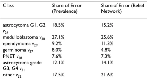
The distribution of the error rate among the classes was approximately the same for both methods of generating prior probabilities, although there were slight differences. Complete results are presented in Table 2. In nearly all incorrectly classified cases, the class with the second high-est posterior probability was the correct class; although this was true for both methods of generating priors. In the incorrectly classified cases, the difference in posterior probability between the predicted label and the correct

Table 2: Breakdown of Classification Errors

Class Share of Error (Prevalence)

Share of Error (Belief Network)

astrocytoma G1, G2 v24

18.5% 15.2%

medulloblastoma v₃₀ 27.1% 25.6% ependymoma v29 9.2% 11.3%

germinoma v₂₇ 8.0% 4.8%

PNET v₂₈ 7.6% 7.3%

astrocytoma grade G3, G4 v31

12.1% 14.1%

other v₃₂ 17.5% 21.6%

Each percentage is the apportionment of total classification errors attributable to each class, obtained over the 920 trials used to estimate the 632+ error.

Part of the complete belief network, showing the locations common to all tumour types but just one tumour classifica-tion path

Figure 2

Part of the complete belief network, showing the locations common to all tumour types but just one tumour classifica-tion path. The complete specificaclassifica-tion, including weights and paths for all tumour types covered is shown in Table 1.

posterior fossa

supra-tentorial

brain stem

IV

ventricle cerebellum cerebrum pineal pituitary lateral ventricle

optic pathway

sella turcica

deep structures

III ventricle 222

631 109631 300631 276702 70267 70221 70217 70299 104702 70267 70251

other area

frontal lobe

occipital lobe

parietal lobe

temporal lobe

optic chiasm

optic

nerve thalamus hypo-thalamus

basal ganglia 4

230 23055 23014 23070 23087 2599 7499 5267 1467 671

medulloblastoma 4

Publish with BioMed Central and every scientist can read your work free of charge "BioMed Central will be the most significant development for disseminating the results of biomedical researc h in our lifetime."

Sir Paul Nurse, Cancer Research UK

Your research papers will be:

available free of charge to the entire biomedical community

peer reviewed and published immediately upon acceptance

cited in PubMed and archived on PubMed Central

yours — you keep the copyright

Submit your manuscript here:

http://www.biomedcentral.com/info/publishing_adv.asp

BioMedcentral label's probability was small (≈ 0.01) for about half the

misclassifications and large (≈ 0.4) for the other half; this was also true for both methods of generating prior proba-bilities.

The simple classifier presented here attempts only to dem-onstrate that the belief network method can be useful and that the data used for its construction is sufficiently accu-rate. The application of the belief network to other classi-fiers depends on the choice of classifier, but many classifiers have a natural way to use prior probabilities either directly or in the form of weights.

Conclusion

Data from a large clinical database, collected over five dec-ades, was used to construct a Bayesian belief network suit-able for generating probabilities of tumour class. The network was shown to enhance a simple probability-based classifier that uses PCA reduced raw MRS spectra for features. It is suggested that additional (discrete) informa-tion could be incorporated into the belief network to fur-ther enhance classifier performance.

Competing interests

The author(s) declare that they have no competing inter-ests.

Authors' contributions

All authors were involved in developing the concept of using prior probabilities in childhood brain tumour clas-sification. GMR constructed the belief networks processed the data and drafted the paper, which was reviewed by TNA and ACP. All authors read and approved the final manuscript.

Acknowledgements

Greg Reynolds holds a Ph.D. studentship funded by the EPSRC. Andrew Peet holds a Department of Health Clinician Scientist Award. The authors wish to acknowledge the help of the West Midlands Regional Childhood Tumour Registry, Birmingham Children's Hospital NHS Foundation Trust, in particular Sheila Parkes for providing the data in a manageable form. We thank the reviewers for their improving comments.

References

1. Preul M, Caramanos Z, Collins D, Villemure J, Leblanc R, Olivier A,

Pokrupa R, Arnold D: Accurate, noninvasive diagnosis of

human brain tumors by using proton magnetic resonance spectroscopy. Nature Medicine 1996, 2(3):323-325.

2. Tate A, Majos C, Moreno A, Howe FA, Griffiths J, Arus C:

Auto-mated Classification of Shot Echo Time in In Vivo 1_{H Brain}

Tumor Spectra: A Multicenter Study. Magnetic Resonance in Medicine 2003, 49:29-36.

3. Lukas L, Suykens J, Vanhamme L, Howe F, Majós C, Moreno-Torres

A, van der Graaf M, Tate A, Arús C, Van Huffel S: Brain tumour

classification based on long echo proton MRS signals. Artifical Intelligence in Medicine 2004, 31:73-89.

4. Devos A, Lukas L, Suykens J, Vanhamme L, Tate A, Howe F, Majos C,

Moreno-Torres A, van der Graff M, Arus C, Van Huffel S:

Classifica-tion of brain tumours using short echo time 1_{H MR Spectra.}

Journal of Magnetic Resonance 2004, 170:164-175.

5. Tate A, Underwood J, Acosta D, Julià-Sapé M, Majós C,

Moreno-Torres A, Howe F, van der Graaf M, Lefournier V, Murphy M, Loose-more A, Ladroue C, Wesseling P, Bosson JL, nas MEC, Simonetti AW, Gajewicz W, Calvar J, Capdevila A, Wilkins P, Bell BA, Rémy C,

Heer-schap A, Watson D, Griffiths J, Arús C: Development of a decision

support system for diagnosis and grading of brain tumours using in vivo magnetic resonance single voxel spectra. NMR in Biomedicine 2006, 19:411-434.

6. Opstad K, Ladroue C, Bell B, Griffiths J, Howe F: Linear

discrimi-nant analysis of brain tumour 1_{H MR spectra: a comparison}

of classification using whole spectra versus metabolite quan-tification. NMR in Biomedicine in press.

7. Galanaud D, Nicoli F, Chinot O, Confort-Gouny S, Figarella-Branger

D, Roche P, Fuentès S, Le Fur Y, Ranjeva JP, Cozzone P: Noninvasive

Diagnostic Assessment of Brain Tumours Using Combined In Vivo MR Imaging and Spectroscopy. Magnetic Resonance in Medicine 2006, 55:1236-1245.

8. de Edelenyi FS, Rubin C, Rubin C, Exteve F, Grand S, Decorps M,

Lefournier V, Bas JFL, Remy C: A new approach for analyzing

proton magnetic resonance spectroscopic images of brain tumours: nosologic images. Nature Medicine 2000, 6:1287-1289.

9. Simonetti AW, Melssen WJ, de Edelenyi FS, van Asten JJA, Heerschap

A, Buydens LMC: Combination of feature-reduced MR

spectro-scopic and MR imaging data for improved brain tumor clas-sification. NMR in Biomedicine 2005, 18:34-43.

10. Luts J, Heerschap A, Suykens J, Van Huffel S: A combined MRI and

MRSI based multiclass system for brain tumour recognition using LS-SVMs with class probabilities and feature selection.

Artificial Intelligence in Medicine 2007, 40(2):87-102.

11. Kleihues P, Burger P, Scheithauer B: The new WHO classification

of brain tumours. Brain Pathology 1993, 3(3):255-68.

12. Russell S, Norvig P: Artifical Intelligence : A Modern Approach New

Jer-sey: Prentice Hall; 2003.

13. Han J, Kamber M: Data Mining : Concepts and Techniques San Francisco:

Morgan Kaufman; 2001.

14. Peet AC, Lateef S, Natarajan K, Sgouros S, Grundy RG: Short Echo

Time 1_{H Magnetic Resonance Spectroscopy of Childhood}

Brain Tumours. Diseases of the Childs Nervous System 2007,

23:163-169.

15. Barkhuijsen H, de Beer R, Ormondt DV: Improved Algorithm for

Noniterative and Time-Domain Model Fitting to Exponen-tially Damped Magnetic Resonance Signals. Journal of Magnetic Resonance 1987, 73:553-557.

16. Efron B, Tibshirani R: Improvements on Cross-Validation: The

.632+ Bootstrap Method. Journal of the American Statistical

Assoca-tion 1997, 92(438):548-560.

Pre-publication history

The pre-publication history for this paper can be accessed here: