~ 277 ~ WWJMRD 2017; 3(7): 277-286
www.wwjmrd.com Impact Factor MJIF: 4.25 e-ISSN: 2454-6615
Safarov Ismail Ibrahimovich
DepartmentHigher mathematics, Tashkent chemistry –technological Institute, Tashkent, Republic of Uzbekistan
Nuriddinov Bakhtiyor Zafarovich
DepartmentHigher mathematics, Bukhara Technological Institute of Engineering, Bukhara, Republic of Uzbekistan
Shodiyev Ziyodullo Ochilovich
DepartmentHigher mathematics, Bukhara Technological Institute of Engineering, Bukhara, Republic of Uzbekistan
Correspondence:
Safarov Ismail Ibrahimovich
DepartmentHigher mathematics, Tashkent chemistry –technological Institute, Tashkent, Republic of Uzbekistan
Dynamic stress - Deformed condition layer cylindrical
layer from the harmonic wave
Safarov Ismail Ibrahimovich, Nuriddinov Bakhtiyor Zafarovich,
Shodiyev Ziyodullo Ochilovich
Abstract
The paper considers an infinitely long circular cylinder consisting, in the general case, of a finite number of coaxial viscoelastic (or elastic) layers, surrounded by a deformed medium. The dynamical stressed - deformed state of a piecewise homogeneous cylindrical layer from a harmonic wave is investigated. Numerical results of stresses are obtained depending on the geometric and physicomechanical parameters of the system.
Keywords: circular cylinder, length of a wave, wave number, stress, deformation.
Introduction
The theory of diffraction of seismic waves is based on the solution of the boundary value problem of the dynamics of a continuous medium. The known number of works with success can be applied to the calculation of underground pipes. These include the work Guz A.N., Kubenko V.D. and Cherevko M.A. [1], which gives an example of calculating the diffraction of a plane harmonic P and SV wave on a rigid circular inclusion soldered into a thin elastic plate. In this case, cases are considered when the inclusion itself is either motionless or it moves together with the plate [2]. The problem of the interaction of an SV wave with a rigid circular inclusion, when on one part of its contour there is complete coherence with the surrounding medium, and on the other - sliding, contact, is solved by Parton V.Z. [3]. The fundamental work devoted to plane waves on a single inclusion is the work of Pao I.Kh. and Mao S.S. [4]. It investigates in detail the diffraction of plane waves of P and SV waves by a rigid and elastic inclusion. An analysis of the example of the calculation carried out by the same authors for a tunnel with concrete lining laid in a granite rock showed that with increasing lining, the tunnel decreases the maximum dynamic pressure; Dynamic stresses exceed the corresponding static by 10 - 15%; at R (where - wave number, R - the outer radius of the inclusion), the dynamic stresses are close to static. It was also shown in [5] that the magnitude of dynamic stresses mainly depends on the ratio of the shear moduli and the propagation velocities of the waves in the soil and in the lining, and also on the thickness of the lining. Similar problems were solved in [6, 7]. All of the above diffraction studies were solved by the method of potentials. In addition to this method, another approach to solving the diffraction problem is known, namely; Method of integral transformations (II P). A major contribution to this field has been made in the works [8,9].
Formulation of the problem.
the j-th viscoelastic layer is enclosed between the j-th and j-th shells. The parameters of the internal and external media are denoted by the indices i=1 and i=N+1. Under
the assumption of a generalized plane-deformed state, the equation of motion in displacements has the form
1)
..N
,
4
,
2
(j
,
~
)
~
2
~
(
22
t
u
b
u
rotrot
u
div
grad
j j j j jj j
1,3...N)
(k
,
t
12
Е
~
-Е
~
-12
Е
~
Е
~
)
1
(
;
t
12
Е
~
Е
~
Е
~
12R
h
1
) ( ) ( 2 2
(k) 2 ) ( 1 4
) ( 4
2 2 к (k) к 3
) ( 3
2 2 к ) ( к
) ( ) ( 2 2
(k) 2 ) ( 1 3
) ( 3
2 2 к ) ( к 2
) ( 2 к 2 к 2
k r к к
k
k k k
k k k
k к к
k
к k k
к
q
w
w
R
h
w
R
h
d
d
q
w
R
h
w
where
j~
,
j~
and
Е
к~
operational Modules of Elasticity
,
)
1
(
,
)
1
(
,
~
;
)
(
)
(
)
(
)
(
~
,
)
(
)
(
)
(
)
(
~
1 1 2 1 2 2 ) ( 2 1
2 2 1 2 )
( 1
01
) ( 0
) ( 0
R
h
с
R
R
R
с
d
t
f
t
R
t
f
E
t
f
E
d
f
t
R
t
f
t
f
d
f
t
R
t
f
t
f
k к k к k к к к
t
E t
i j
j
t i j
j
Here
u
j
u
rj,
u
j
- displacement vector, which depends от
r
,
,
t
;j- density of the layer material;)
(
t
f
– some function;R
Е(i)(
t
),
R
(i)(
t
)
and)
(
)(
t
R
i - relaxation core;
oj,
oj- instant elastic moduli of the viscoelastic layer,E
01- instantaneous elasticity moduli of the shell. At pressures up to 100 MPa, the motion of the liquid is satisfactorily described by the wave velocities for the potentials of the liquid particles [11]2 0 2
2 0
1
t
С
о
, (2)where Со – acoustic velocity of sound in a liquid. Potential
0
and the velocity vector of the liquid are related by the dependence
V
grad
0. Fluid pressurer
R
0 is determined by means of the linearized Cauchy-Lagrangeintegral
t
С
Р
о
00
– the liquid pressure on thewall of the cylindrical layer and ρо – density of the liquid.
Under the condition of continuous flow around a fluid, the normal component of the velocity of the liquid and the layer on the contact surface r = R1 should be equal
1 1
1 0
R r r
R
r
t
u
r
, (3)
where
u
r1 – moving the layer along the normal.The problem is solved in the displacement potentials, for this purpose we represent the displacement vector in the form:
)
1
...
4
,
2
(
,
grad
rot
j
N
u
j
j
j , (4)where
j – longitudinal wave potential;
j(
rj,
j)
– vector potential of transverse waves
t
j j j
j oj j oj
j j t
j j
oj t
j j
oj j oj oj
t
d
t
R
t
d
t
R
d
t
R
2 2 2
2
2 2 2
2 2
)
5
(
2
2
where
2 2
2 2
2
2
1
1
r
r
r
r
– Differentialoperators in
Cylindrical coordinates and
v
j – Poisson's ratio [12]. The potential for the external region can be represented in the form) (
1 ) (
1 1 )
( 1 ) (
1
1
,
s N p N N s
N p N
N
, (6)where ( ) 1 )
( 1
,
p N p
N
– determine the unperturbed stress field; Field in the absence of any surface heterogeneity;) (
1 ) (
1
,
s N sN
- the stress field due to the presence of a cylindrical surface. In [14] a generalization of the Lamb results was obtained and it was found that a non-perturbed field is determined,
)
(
)
sin(
;
)
(
)
cos(
(1) 111 1 2
) (
1 1
1 ) 1 ( 1 1 1
) (
1
t i N p
N t
i N p
N
F
H
r
e
F
H
r
e
(7)where
,
/
;
/
,
4
/
;
4
/
2 ) 1 ( 2 2
1 2
) 1 ( 2 2
1
) 1 ( 2 1 2
) 1 ( 1 1
N s N
N p N
N s N N
р N
c
c
c
ip
F
c
iр
F
and the quantity НN (Z) Is a Hankel function of the first
kind and of order . Using the addition theorem for Bessole functions [15], expressions (8) can be rewritten in the form
) ,... 2 , 1 ( 0 ,
0
)] sin(
) ( ) ( ) 1 ( [
)] (
) ( ) ( ) 1 ( [
) ( ) (
1 ) 1 (
1 1 1
2 )
( 1
1 ) 1 (
1 1 1
) (
1
N j
e m Z
H r J F
e m сos Z H
r J F
p j p j
t i N
m N m m m
p N
t i N
m N m m m
p N
(8)
where Jm- Bessel function of the first kind of order m. On
t i N m m N m N m s N t i N m m N m N m s N t i j m jm t i j m jm jm jm m s j t i j m jm j m jm jm jm m s j
e
r
H
m
D
m
C
e
r
H
m
B
m
А
e
r
H
D
e
r
H
C
m
D
m
C
e
r
H
B
r
H
А
m
B
m
А
)
(
)
cos(
)
sin(
(
)
(
))
cos(
)
sin(
(
))
(
)
(
)(
cos(
)
sin(
(
))
(
)
(
))(
sin(
)
cos(
(
1 ) 1 ( ) 1 ( ) 1 ( ) ( 1 1 ) 1 ( ) 1 ( ) 1 ( ) ( 1 ) 2 ( ) 1 ( ) ( ) 2 ( ) 1 ( ) ( (9)where
А
jm,
B
jm,
C
jm,
D
jm,
А
jm,
B
jm,
C
jm,
D
jmconstants to be determined from the contact conditions r=Rn. (n=1,2,3,…N) the construction of a formal solution
does not encounter fundamental difficulties, but the investigation of such a solution requires a huge amount of computation. Problems are reduced to solving non-homogeneous algebraic equations with complex coefficients
[c]{g}={p} (10)
In the case when E1=E2…=EN, 1=2…=N and
1=2…=N, we obtain holes in an infinitely elastic
medium. In this case the boundary is stress-free. The unknown constants from (11) are determined by the formulas:
,
)
1
(
sin
,
)
1
(
cos
,
)
1
(
cos
,
)
1
(
sin
Nm m Nm Nm m Nm Nm m Nm Nm m NmА
C
B
А
(11) where).
(
)
(
)
1
(
);
(
)
(
]
2
[
);
(
)
(
]
2
[
;
;
/
}]
){
(
[
}
){
(
[
;
/
}]
){
(
[
}
){
(
[
1 ) 1 ( ) 1 ( 2 2 2 1 2 2 2 1 2 1 2 1 2 1 1 N N m N N N N m Nm N N m N N N N m N N Nm N N m N N N N m N N Nm mk mk mn mk m m mk mn mk mk N m mk mn mk mk N m Nm m mа mа ma mk N m mk mn mk mk N m NmR
J
R
R
J
m
m
E
R
H
R
X
R
H
R
m
m
D
R
J
R
X
R
J
R
m
m
D
F
K
K
D
E
K
D
K
Z
H
F
D
E
E
D
Z
H
F
K
K
K
H
Z
H
F
K
D
K
E
Z
H
F
In this case, the circumferential stress on the cavity surface
is reduced to the following:
4
1
1
1
(1)
cos
,
0 2 0
2 i t
n o n n n n i
i
H
r
T
n
D
e
R
t
R
where
2 1 2 1 2 1 1 ) 1 ( 2 1 2 2 1 1 1 ) 1 ( 1 1 2 1 1 ) 1 ( 1 2 1 2 2 1 2 1 2 1 1 1 1 1 2 1 2 3 1 1 1 1 1 1 1 1 1 1 1 1 1 1/
,
)
2
1
(
)
1
(
)
4
1
(
)
2
1
(
S p n n n n n n n n т тC
C
R
R
H
R
n
n
R
H
R
n
R
H
R
R
n
n
R
H
R
R
n
n
R
Q
R
Q
R
H
R
H
R
R
Т
Т
Coefficient of voltage concentration
is defined as follows 1 1 1 R r r r R r R r
(12)
where
rr is defined as a function (р) as
rr= i 0 2 [ H2(1)((r
)
+(1-R2) Ho(1)()
r
] e-itTo solve the system of equations (11), in general, the Gauss method is used, with the separation of the principal element.
,
sin
)
(
)
(
)
(
)
(
,
sin
)
(
)
(
,
cos
)
(
))
(
(
)
(
)
(
,
)
(
)
(
0 2 ) 2 ( 2 2 ) 1 ( 1 2 ) 2 ( 1 ) 1 ( 2 0 1 ) 1 ( 1 1 ) 1 ( 1 0 2 ) 2 ( 2 ) 1 ( 2 ) 2 ( 2 2 ) 1 ( 2 2 0 1 ) 1 ( 1 ) 1 ( 1 1
n n n n n n n n n Q n n n n n Q n n n n n n n n n n r n n n n rm
r
H
L
r
H
D
r
h
H
r
n
C
r
h
H
r
n
u
B
r
H
A
r
h
H
r
n
u
M
r
H
r
n
r
H
r
n
L
D
r
h
H
h
C
r
h
H
h
u
r
H
r
n
A
r
h
H
h
u
where h 1= p/cp1, 1 = p/cs1,
h2 = p/cp2, 2 = p/cs2,
;
sin
)
,
(
1
)
(
2
)
(
2
)
(
2
)
(
cos
)
,
(
1
)
(
'
2
)
(
'
2
)
(
)
2
;
cos
)]
,
(
1
)
(
[
2
)
(
2
)
(
cos
)]
,
(
1
)
(
[
2
)
(
2
)
(
) 1 ( 1 )' 1 ( 1 1 1 ) ' 1 ( 1 1 ) 1 ( 2 2 2 1 2 1 1 ) 1 ( 1 ) 1 ( 1 1 ) 1 ( 1 1 ) 1 ( 2 2 1 2 1 1 1 ) 1 ( 0 ) 1 ( 1 ) 1 ( 1 2 1 1 ) '' 1 ( 1 1 ) 1 ( 2 1 2 0 ) 1 ( 1 ) 1 ( 1 2 1 1 ) '' 1 ( 1 1 ) 1 ( 1 1 ) 1 (
n n n n n n s n n n n n n n n n n n n n n n n n n n n rrB
r
H
r
r
H
r
h
A
r
h
H
r
h
r
h
H
r
n
h
r
k
C
B
r
H
r
r
H
e
r
n
А
r
h
H
h
r
r
h
H
r
n
h
B
r
e
H
r
r
e
H
e
r
n
А
h
r
h
H
h
r
h
H
h
B
r
e
H
r
r
e
H
t
r
n
А
h
r
h
H
h
r
h
H
where 2 1
, thenElements of the matrix [C] (10) have the following form:
(
)
(
)
;
1
1 1 1 1 1 113
nH
h
b
h
bH
h
b
b
С
n
n
(
)
(
)
;
1
2 1 ) 2 ( 2 2 ) 2 (14
nH
h
b
h
bH
h
b
b
С
n
n
(
)
(
)
;
);
(
);
(
);
(
2 16 (2) 2 21 (1) 2 22 (1) 1 1 (1) 1 1) 1 (
15
nH
b
bH
b
b
n
С
b
h
H
b
n
С
b
H
b
n
С
b
H
b
n
С
n
n
n
n
n
(
)
(
)
;
1
;
)
(
)
(
1
);
(
);
(
2 1 ) 2 ( 2 2 ) 2 ( 26 2 1 ) 1 ( 2 2 ) 1 ( 25 2 ) 2 ( 24 2 ) 1 ( 23b
bH
b
nH
b
С
b
bH
b
nH
b
С
b
h
H
b
n
С
b
h
H
b
n
С
n n n n n n
)
(
2
)
(
(
2
2
;
)
(
2
)
(
(
2
2
;
)
(
2
)
(
(
2
2
2 1 ) 2 ( 2 2 ) 2 ( 2 2 2 1 2 2 1 34 2 1 ) 1 ( 2 2 ) 1 ( 2 2 2 1 2 2 1 33 1 1 ) 1 ( 1 1 ) 1 ( 2 2 2 1 2 2 1 31b
h
H
b
h
b
h
H
b
b
n
n
n
K
С
b
h
H
b
h
b
h
H
b
b
n
n
n
K
С
b
h
H
b
h
b
h
H
b
b
n
n
n
K
С
n n n n n n
(
1
)
(
)
(
)
;
2
(
1
)
(
)
(
)
;
2
*
(1) 2 2 (1) 1 22 35 1 1 ) 1 ( 1 1 ) 1 ( 2 1
32
n
H
b
bH
b
b
n
С
b
bH
b
H
n
b
n
С
n
n
n
n
(
1
)
(
)
(
)
;
2
(
1
)
(
)
(
)
;
2
;
)
(
)
(
)
1
(
2
*
;
)
(
)
(
)
1
(
2
2 1 ) 2 ( 2 2 ) 2 ( 44 2 1 ) 1 ( 2 2 ) 1 ( 2 43 1 1 ) 1 ( 1 1 ) 1 ( 2 1 41 2 1 ) 2 ( 2 2 ) 2 ( 2 36b
h
bH
h
b
h
H
л
b
т
С
b
h
bH
h
b
h
H
k
b
n
С
b
h
bH
h
b
h
H
n
b
n
С
b
bH
b
H
n
b
n
С
n n n n n n n n
(
)
(
)
;
0
.
)
(
2
;
)
(
)
(
)
(
2
;
)
(
)
(
)
(
2
52 51 2 1 ) 2 ( 2 1 ) 2 ( 2 2 ) 2 ( 2 2 2 2 2 46 2 1 ) 2 ( 2 1 ) 1 ( 2 2 ) 1 ( 2 2 2 2 2 45 2 1 ) 1 ( 2 1 ) 1 ( 1 1 ) 1 ( 2 2 2 2 1 42
С
С
b
e
H
b
e
H
b
e
b
e
H
b
n
b
e
С
b
e
H
b
e
H
b
e
b
e
H
b
n
b
e
С
b
e
H
b
e
H
b
e
b
e
H
b
n
b
e
С
n n n n n n n n nHow С33 at С53= -С33 with an argument С53(h2)= -
С33(h2b)
);
(
2
)
(
)
(
2
2
2 (1) 2 2 (2) 1 22 2 2 2 2 2 2
53
h
H
h
h
H
h
n
n
K
С
n
n
2 1 ) 2 ( 2 2 ) 2 ( 2 2 2 2 2 2 2 2 54(
2
)
(
)
(
2
2
n
n
h
H
h
h
H
h
K
С
n
n
),and in the case of С55(2) = С55(2b)
(
)
(
)
;
)
(
2
;
)
(
)
(
)
(
2
);
(
)
(
;
)
(
)
(
)
1
(
2
;
)
(
)
(
)
1
(
2
)
(
)
(
0
;
)
(
)
(
)
1
(
2
;
)
(
)
(
)
1
(
2
2 1 ) 1 ( 2
1 ) 1 ( 1 2 ) 2 ( 2
2 2 2 2 66
2 1 ) 1 ( 2
1 ) 1 ( 1 2 ) 1 ( 2
2 2 2 2 65
2 45 2
65
2 1 ) 1 ( 2 2 ) 1 ( 2
64
2 1 ) 1 ( 2 2 ) 1 ( 2
63
2 43 2
62 62 61
2 1 ) 2 ( 2 2 ) 2 ( 2
56
2 1 ) 1 ( 2 2 ) 1 ( 2
55
n n
n
n n
n
n n
n n
n n
n n
H
H
b
H
n
С
H
H
H
n
С
b
С
С
h
H
h
h
H
n
n
С
h
H
h
h
H
n
n
С
b
h
C
h
С
С
С
H
e
H
n
n
С
H
H
n
n
С
Thus, we can find the elements of the matrix [C] for any order
);
(
)
(
)
2
(
);
(
)
(
)
2
(
);
(
)
(
)
1
(
);
(
)
(
)
1
(
);
(
)
(
)
1
(
1 2
2 2
1 1 / 1
/ / 2
2 2
1 1
1 )
1 (
R
RH
R
H
R
m
m
m
K
R
RJ
R
J
R
m
m
m
K
R
RH
R
H
m
m
K
R
RJ
R
J
m
m
H
R
H
R
R
H
m
m
E
n m n n
m N
mk
n n m n n n
n n m n n
n mk
n m n n n m mk
N m N
m mk
N m m N N
m mk
The most obvious criterion for assessing the deterministic state is the choice of the "concentration coefficient" (stresses, deformations, etc.). The main objectives of this work are:
A) study of the redistribution of stresses due to the presence of a cavity or inclusion;
B) a study of the effect of the location of the source of excitation on this distribution. In accordance with such problems, stress concentration coefficients К1N, К2N, К3N
and К4N are determined by the voltage:
)
,
,
,
(
,
,
,
1 2 3 42 ) (
2
2 ) (
1
2 ) (
2
1 )
( n n n n
n p
n
n p
n
n p
n
n p
n
K
K
K
K
Here
(
1n,
2n)
и
(
(К)1n,
(К)nN)
- the main stresses, determined by the potentials (,) and ((Р), (Р)). The principal stresses are related to the components of the plane stress state by the following relations [16].
1,2=0,5{(rr+)[(rr-)2+4r2)]1/2}
it is also possible to determine the strain energy concentration coefficient, defined by expression:
(N /tn (p)) r=Rn = sn / sn(p) = K(n) s
where S and S(H) – Functions of the deformation energy plane for the same point, related to the displacement potentials. (1y) and ((n)(n)). The energy density of the
strain is expressed in terms of the principal stresses: EN=[21n+22n-2vn1n+2n]/(2En) ,
where EN and n respectively, Young's modulus and the
Poisson's ratio.
Solutions (4) and (5) define complex stresses. Consequently, the functions of the deformation energy plane have the form:
( T+iImT)e2iωt=[(ReT)2+(imT)2]1/2е-i(2ωt-1)
T(p)(ReF(p)+iImT(p))e2iωt=[(ReT(p))2+(imT(p))2]1/2e-i(2ωt-), where 1n= rc tg(ImT/ReT), 2 = rc tg(Im(T (p)
)/(ReT(p))). Thus, the quantity
) 1 ( 2 / 1
2 ) ( 2
) (
2 2
2
)
(Im
)
(Re
)
(Im
)
(Re
i n тp p
т
e
S
S
S
S
K
(13)Does not depend on time and is complex. As a measure of concentration, we can choose the value [16]
2 / 1
2 ) ( 2
) (
2 2
)
(Im
)
(Re
)
(Im
)
(Re
/
/
т p pc
S
S
S
S
K
S
(14)Notice, that
Scn=Sc(,n, n, n; Z, n, Rn, n).
Е = Е1/Е2 , density ratios = 1/2 , geometric parameters
R1 and R2. If all the characteristics (Fig. 1) of the
mechanical system are the same (Е1=Е2=. . . Еn; 1 = 2 =.
. .= n ; 1 = 2 = 3 =. . . = n) , Then the problem of the
interaction of cylindrical waves with cylindrical cavities. In the particular case, the solutions obtained for the cavity coincide with the solutions of RS. Moop and W. N. Rao [2]. The results of calculations of the stress concentration are shown in Fig. 2. From the analysis of numerical results in Fig. 2. It can be seen that , R, and n The stress concentrations of the rim face coincide. In the particular case, we consider the interaction of waves with a rigid inclusion (Fig. 1), then on the boundary r =R1 The
following conditions are imposed:
sin
cos
u
U
U
u
r
(15),
)
sin
cos
(
)
(
12
0 2
1
1
R
U
R
d
R r r
rr вкл
where On – inclusion density.
It is found that the transfer and rotation of the inclusion as a rigid integer are determined by the expressions:
U=-
e
iwt
[F1cosyH2 (1Z)J1(1R1)-F2cosyH2(1Z1)J1(1
R1)-C1H1(1 R1)+
+F1cosyH0 (1Z)+J-1(1R1)+F2cosyH0(1Z)J-1(1 R1)-
- N-1H-1(1R1)+C-1H-1(1R1)],
V=-iwt
N
e
R
[-F1sinH2(1Z)J1(1R1)+F2sinyH2(1Z1)J1(1R1)-
A1H1(1R1)+
+D1H-1 (1R1)+F1sinyH0(1Z)J-1(1R1)+F2sinyH0(1Z)J -1(1R1)+
+A-1H-1(1R1)+D-1H-1(1R1)];
=-iwt
e
24
[F2sinyH1(1Z1){J0(1R1)+ N N
R
2
J -1(1R1)}+D{H0(1R1)+
+ N N
R
2
H-1(1R1)}],
where U, V – In the directions of x and y respectively, - angle of rotation, =рср/рon. . The solutions of equation
(15) are expressed in terms of the Bessel and Hankel functions of the first and second kind of the n-th order. Of special interest is the case of a fixed inclusion, i.e. =0. For this inclusion, the conditions on r = RN have the form:
U=V==0; ur=u=0.
It can be verified that from the motion the inclusion is held by the forces X and Y in the directions x and y respectively and the moment M in the x-y plane, which are defined by formulas
Х
=P2Rn2cos(g+h)e-iwt,Y
=P2Rn2sin(-g+h)e-iwtN
R
M
=-P2R12sinH1(1Z)
0 1 1 1 1
1
(
)
V
R
H
R
e-iwt where =P/Rn1 , 1=(1-v
2
1)/(21R1) ,2=(1+v 2
1)/1R1.
,
2
1
)
(
4
1
,
2
1
)
(
4
1
1 1 1
1 0
1 1 1
1 02
1
1 1 1
1 1
1 1
1 2
1
V
a
H
a
aH
z
H
a
V
a
H
a
aH
z
H
a
h
V
a
aH
a
H
z
H
a
V
a
H
a
aH
z
H
a
g
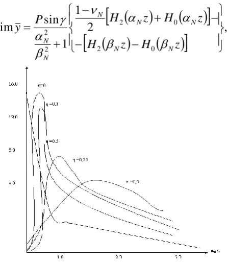
Using suitable expansions for the Hankel function, it can be shown that
2
,
1
1
sin
lim
0 2
0 2
2 2
z
H
z
H
z
H
z
H
P
y
N N
N N
N
N
N
Fig. 3: Dependence of the energy concentration coefficient on
the wave number 1R1 (r1/D=3,5)
2
,
1
1
cos
lim
1 0 1
2
1 0 1 2
2 2
z
H
z
H
z
H
z
H
P
x
N
N
N
0
0
lim
aM
Some graphs of the nature of stress redistribution near the discontinuity surface are given. Figures 2 and 3 give graphs of the coefficient Sc as a function 1 R1 for
different values and . These graphs show that for given
, and there is a value 1R1=, which maximizes the
value Sc. The propagation of waves from a source
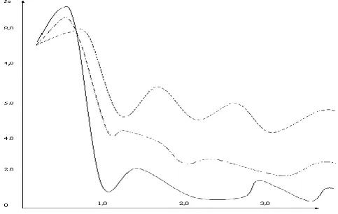
О
Fig. 4: Dependence of the energy concentration coefficient on the wave number (v=0.25).
In the following example, we consider the interaction of cylindrical waves with a cylindrical layer (the boundary conditions at the contact of the layer (r = R2) and free
surface (
= Ri) are given in (11). From the generalsolutions we obtain solutions for n = 1,2. The numerical
results are shown in Fig. 3.4. From Fig.3.4. It is clear that the concentration of the voltage depends essentially on the location of the harmonic wave source. When ro / D = 2 the
dynamic concentration curve differs from static to 15%. When 1P1=2 the results of the static and dynamic stress
state are radically different for close ro /D = 2 source
distances. Now we consider some limiting cases. Here are the results for the hole. If in equation (15) ro Tends to
infinity, then we can use the asymptotic expansions of the Hankel function for large values of the argument.
0
1 1
2
cos
1
1
4
4
lim
1
m
t i m n m R
r o
r
C
S
e
k
o
- конечное .
This expression completely coincides with the expressions obtained [18] for a plane incident wave. Defining an asymptotic static solution, we obtain
2
2 1
0 2 1
cos
)
1
(
)
(
cos
4
)
(
1
4
lim
1
m
m
o o
R r
o
m
m
r
R
r
r
R
r0 - final.
This solution exactly coincides with the solution of the static problem obtained by [17].
The difference between the results obtained in the present paper and the results of the ordinary wave diffraction problem justifies their consideration in many practical problems.
Table 1
R1/ro 3 4 5 50 60 80
Θ, Hailstones 60о 70о 90о 90о 90о 90о |σθθ| 1,541 1,536 1,525 1,414 1,416 1,416
Table 1 shows the stress concentrations as a function of R1/ro for different values of θ. It can be seen that the
maximum stress |σθθ| in a cylindrical body arises when θ
= 30о (σθθ = σ θθ/ σкк) . At R1/ro > 50 The impact of a
cylindrical source is decomposed as a plane wave, i.e. The radius of curvature of the wave can be ignored.
Conclusions
1. The problem of diffraction of harmonic waves in a cylindrical body is solved in displacement potentials. The displacement potentials are determined from the solutions of the Helmholtz equation. Arbitrary constants are determined from the boundary conditions that are placed between the bodies. As a result, the problem posed reduces to a system of inhomogeneous algebraic equations with complex coefficients that are solved by the Gauss method with the separation of the principal element.
2. Contour stresses σθθ on the free surface of cylindrical
bodies reach their maximum value in 1.
waves
al
longitudin
of
action
Under the
4
s
shear wave
of
action
Under the
2
Q
2. Contour stresses σθθ under the action of transverse
harmonic waves is 15-20% greater than when exposed to longitudinal waves.
3. When the source of harmonic waves is at a distance of five radii (
V
5
R
) from the cylindrical body, the high-frequency nature of the change in contour stresses σθθ, Acting on the internal free surface, canbe approximated well by the solution for a flat (
V
) wave. Further, all values approach the same asymptote.4. Numerical results show that the dynamic stress concentration coefficients around cylindrical bodies depend on
A) the distance between the source and the body; B) the wave number for the sphere and the body; C) physicomechanical parameters of the sphere and body; In the case of a cavity in an unbounded medium, the loop voltage depends on:
A) the distance between the source and the cavity; B) the wave number;
C) Poisson's ratio of the medium.
References
1. Guz A.N., Kubenko V.D., Cherevenko M.A. Diffraction of elastic waves. "Nauk", 1978. 308 p. 2. Pao Y.H., Mow C.C. Diffraction of elastic waves and
dynamic stress concentration. No. 4, Grane, Russak, 1973 694 p.
4. Datta S.K. Tensional waves in an infinite elastic solid containing a penny – shaped crack.-z. answer. Math. And Phys., 1970, 21, №3, р.343-351
5. Mubarikov Ya.N., Safarov I.I. On the effect of an elastic wave on a cylindrical shell. Izv.AnuzSSR, series of engineering sciences, 1987. №4. P. 34-40 6. Safarov I.I. Estimation of the seismic stress of
underground structures of the wave dynamics method. Collection "Seismodynamics of tasks and structures" Tashkent, Fan. 1988.
7. Filippov I.G. , Egorychev OA Nonstationary oscillations and diffraction of waves in acoustic and elastic media. . - M .: Mechanical Engineering, 1977.-304 p.
8. Safarov I.I. Interaction of waves in multilayered cylindrical layers in an infinite elastic medium. Proceedings of VII All Union. Conference "Basic Dynamics, Foundations and Underground Structures" Dnepropetrovsk, 1989. p. 56-57
9. Safarov I.I., Zhumaev Z.F. On the destruction of the tunnel with strong movements of the earth. International Conference on Earthquake Engineering. S-Petrburg, 2000, p. 71-78
10. Avliyakulov N.N., Safarov I.I. Modern problems of statics and dynamics of underground pipelines. Tashkent, Fan va texnologiya. 2007. 306 pp.
11. Bozorov M.B., Safarov I.I., Shokin Yu.I. Numerical simulation of oscillations of dissipatively homogeneous and inhomogeneous mechanical systems. Novosibirsk: Izd. Of the SB RAS. 1996.189 p.
12. Rashidov T.R., Safarov I.I. And others. Two main methods of studying the seismic stress of underground structures under the action of seismic waves. Tashkent: DAN. № 6, 1989. p. 13-17.
13. Safarov I.I. Auliyakulov N.N. Methods of increasing the seismic resistance of underground plastic pipelines // Uzbek Journal of Oil and Gas, 2005, №4. p.42-44. 14. Safarov I.I., Teshaev M.Kh. , Kilichev O. Dynamic
stressed states of thin-walled pipelines. LAP, Lambert Academic Publishing (Germany). 2016. 230p.
15. Safarov I.I., Teshaev M.Kh. Akhmedov M.Sh. Stress-deformed states of thin-walled pipelines. Lambert Academic Publishing (Germany). 2015. 335p.
16. Safarov I.I, Boltaev Z. I., Akhmedov M. Sh. Properties of wave motion in a fluid-filled cylindrical shell/ LAP, Lambert Academic Publishing . 2016 -105 р.
17. Safarov I.I, Akhmedov M. Sh.,Qilichov O. Dynamics of underground hiheline from the flowing fluid. . Lambert Academic Publishing (Germany) . 2016. 345р.