1
Zero-dimensional transient model of large-scale cooling
1ponds using well-mixed approach
23
Ahmed Ramadan1*, Reaz Hasan2, Roger Penlington3
4
1, 2, 3 Northumbria University at Newcastle, Department of Mechanical and Construction
5
Engineering, Newcastle upon Tyne, NE1 8ST, UK. 6
* corresponding author: Ahmed Ramadan: Fax: +44 191 232 6002 E-mail address: 7
9
Abstract
10Nowadays, nuclear power plants around the world produce vast amounts of spent fuel. After 11
discharge, it requires adequate cooling to prevent radioactive materials being released into the 12
environment. One of the systems available to provide such cooling is the spent fuel cooling 13
pond. The recent incident at Fukushima, Japan shows that these cooling ponds are associated 14
with safety concerns and scientific studies are required to analyse their thermal performance. 15
However, the modelling of spent fuel cooling ponds can be very challenging. Due to their large 16
size and the complex phenomena of heat and mass transfer involved in such systems. In the 17
present study, we have developed a zero-dimensional (Z-D) model based on the well-mixed 18
approach for a large-scale cooling pond. This model requires low computational time compared 19
with other methods such as computational fluid dynamics (CFD) but gives reasonable results 20
are key performance data. This Z-D model takes into account the heat transfer processes taking 21
place within the water body and the volume of humid air above its surface as well as the 22
ventilation system. The methodology of the Z-D model was validated against data collected 23
from existing cooling ponds. A number of studies are conducted considering normal operating 24
conditions as well as in a loss of cooling scenario. Moreover, a discussion of the implications 25
of the assumption to neglect heat loss from the water surface in the context of large-scale ponds 26
is also presented. Also, a sensitivity study is performed to examine the effect of weather 27
2
Keywords: Spent nuclear fuel, large-scale cooling ponds, analytical modelling, well-mixed 29
approach, transient heat transfer. 30
Nomenclature
𝐴 surface area (m2) 𝑦 mole fractions
𝐶𝑝 specific heat capacity at constant
pressure (J/kg K)
∆𝑡 time step size (s)
𝐶𝑤 specific heat capacity of water (J/kg
K) Greek symbols
ℎ𝑐 convection heat transfer coefficient
(W/m2 K)
𝜀 emissivity
ℎ𝑐𝑜𝑛 condensation mass transfer
coefficient (m/s)
𝜌 density (kg/m3)
ℎ𝑒𝑣 evaporation mass transfer coefficient
(m/s)
𝜎 Stefan-Boltzmann constant (W/m2 K4)
ℎ𝑣(𝑇) enthalpy of vapour at a given
temperature (kJ/kg) Subscripts
ℎ𝑓𝑔 latent heat of vaporisation for water
(kJ/kg)
𝑎 dry air
𝑘 thermal conductivity (W/m K) ∞ ambient
𝑚 mass (kg) 𝑐 convection
𝑚̇ mass flow rate (kg/s) 𝑐𝑜𝑛 condensation
𝑀 molecular weight (kg/kmol) 𝑑 heat load
𝑁 mole number (kmol) 𝐷 designed value
𝑁̇ molar flow rate (kmol/s) 𝑒𝑣 Evaporation
𝑁𝑢 Nusselt number ℎ hall
𝑃 pressure (Pa) 𝑙 leakage
𝑄̇ heat transfer rate (W) 𝑚 make-up
𝑅𝑎 Rayleigh number 𝑝 pond
𝑅𝐻 relative humidity (%) r radiation
𝑅𝑜 universal gas constant (J/K kmol) 𝑅 rack
𝑆ℎ Sherwood number 𝑠𝑎𝑡 saturation
𝑇 temperature (K) 𝑡 total
𝑉 Volume (m3) 𝑣 vapour
𝑥 wall thickness (m) 𝑣𝑒𝑛𝑡 ventilation
𝑤 water
3
1
Introduction
31
In the past decades, increasing the use of nuclear power for electricity generation has gained a 32
lot of attention amongst scientists. Nuclear reactors around the world are now discharging a 33
massive amount of spent nuclear fuel, which is predicted to reach approximately 445,000 t HM 34
(metric tonnes of heavy metal) by 2020 [1]. This includes 69,000 t in Europe and 60,000 t in 35
North America. Despite the recent incident at Fukushima, Japan [2], nuclear power generation 36
continue to grow in developed countries, as evidenced by the recent massive investment in 37
nuclear energy by the UK government in approving an £18bn nuclear plant at Hinkley Point 38
C. This will deliver 7% of Britain’s electricity needs for the next six decades [3]. 39
The issue of long-term storage was not considered when the original decisions were made 40
regarding the fuel cycle [4]. Recently, waste management has become one of the major policy 41
issues in most nuclear power programmes. Meanwhile, the options chosen for waste 42
management can have extensive effects on political debates, propagation risks, environmental 43
threats, and economic costs of the nuclear fuel cycle. This increases the significance of 44
modelling the cooling ponds and analysing their performance to provide a better understanding 45
of their pond thermal behaviour. This will allow for better operation and could offer mitigation 46
options whenever needed in accident scenarios. 47
Several research investigations have considered the thermal-hydraulic behaviour of the spent 48
fuel cooling ponds, which are mainly focused on accident scenarios and their consequences [2, 49
5-8]. These studies used two main modelling approaches. The first approach is the use of so-50
called system codes such as RELAP, TRACE, ATHLET, MELCOR and ASTEC. These codes 51
are based on dividing the system into a network of pipes, pumps, vessels, and heat exchangers. 52
Mass, momentum and energy conservation equations are then solved in one-dimensional form. 53
Many phenomena and physical behaviour such as two-phase flows and pressure drop due to 54
friction rely on empirical correlations. These codes are suitable for systems that can be 55
represented by one-dimensional flows. However, when such a system involves multi-56
dimensional phenomena, these codes do not provide a good approximation. Some attempts 57
have been made to improve their capability to handle multi-dimensional flows. One of these 58
attempts considers the system as an array of parallel one-dimensional pipes, where the 59
interaction between them is allowed through cross-flow coupling. Although they provide 60
4
not offer appropriate descriptions of multi-dimensional flows. The MARS code is an example 62
of attempts to include a multi-dimensional analysis capability in system codes [9]. 63
The second approach is a numerical method such as computational fluid dynamics (CFD) 64
which in principle can address details of thermos-fluid phenomena in cooling ponds Numerical 65
methods such as CFD can be used, in principle, to address fluid flow and heat transfer scenarios 66
in three dimensions using computers. The CFD methodology is now well-established, but the 67
available literature indicates that a full CFD model of a spent fuel cooling pond may be not 68
practically possible. This is due to their large size and the existence of complex phenomena, 69
such as evaporation, which requires multiphase flow models. However, some studies have 70
reported CFD modelling of spent fuel ponds taking into account only the water body without 71
considering the humid air zone above or ventilation and their effect on the evaporation rate. 72
Also, some of the challenges encountered during the CFD simulation have been discussed in 73
our previous work [10]. An example of the use of CFD in improving the safety of such cooling 74
ponds can be found in a study conducted by Ye et al. [11], in which a new passive cooling 75
system was designed to provide an adequate cooling for the CAP1400 spent fuel pool in 76
emergency situations. Hung et al. [12] used the CFD approach to predict the cooling ability of 77
the Kuosheng spent fuel pool and to confirm that the existing configuration can provide enough 78
cooling to meet licensing regulations with a maximum water temperature of 60 °C. A unique 79
aspect of their work is that they used CFD in a more advanced way than in other studies to 80
predict local boiling within the pool water, reflecting the strength of the CFD approach. 81
Another use of CFD is to study flow characteristics within fuel assemblies. For example, a 82
study conducted by Chen et al. [13] investigated flow and heat transfer within a rod bundle 83
using a three-dimensional model. 84
Yanagi et al. [14] produced a CFD model for a cooling pond and compared the predicted water 85
temperature with those for the cooling pond at Fukushima Daiichi Nuclear Power Station under 86
loss of cooling conditions. The water surface was modelled using a previously derived heat 87
transfer correlation by the same authors [15]. The CFD model produced by Yanagi et al. [14] 88
was further used to form a baseline for an analytical model "One-Region model" also generated 89
by Yanagi et al. [16, 17]. This One-Region treats the water as on node with a single temperature 90
value without taking into considerations its distribution. After that, they have examined the 91
effect of the distribution of the heat load on the variation of water temperature and it was 92
confirmed that the One-Region model applicable to predict the water temperature in the cooling 93
5
On the other hand, most of the studies adopting the system codes were concerned about 95
investigating accident scenarios and their consequences. Carlos et al. [18] used the TRACE 96
best estimate code to analyse the safety of the Maine Yankee spent fuel pool. Ognerubov et al. 97
[19] investigated scenarios of the loss of water in a spent fuel pool in the Ignalina NPP using 98
various system codes to identify potentially unrealistic parameters while performing the 99
calculations. Groudev et al. [20] used RELAP5 to study the thermal-hydraulic behaviour of 100
spent fuel for a dry out scenario while transferring fuel from the Kozloduy NPP reactor vessel 101
to the cooling pool. Additional studies dealing with fuel ponds can be found elsewhere [5, 21, 102
22]. 103
Some investigations concern accident mitigation options using thermal-hydraulic codes. Chen 104
et al. [6] used the GOTHIC code to model a spent fuel pool owned by the Taiwan Power 105
Company to analyse its response to spray mitigation under loss-of-coolant scenarios. Wu et al. 106
[23] conducted an analysis of the loss of cooling accident scenarios for a spent fuel pool at the 107
CPR1000 NPP using the MAAP5 code. In the same study, the authors discussed mitigation 108
measures to recover the pool cooling system using make-up water. 109
The literature cited above shows that the CFD approach is more convenient when it comes to 110
improving the design of cooling ponds, as it offers an in-depth understanding of heat and mass 111
transfer and fluid mixing. On the other hand, thermal-hydraulic system codes such as TRACE 112
are more suitable for analysing safety issues with such ponds and when the system under 113
consideration can be approximated to one-dimensional flow. 114
In general, most studies focus on investigations of severe accident scenarios and the analysis 115
of their consequences. However, relatively few studies have reported on improving pond 116
design as well as accident mitigation options. Conversely, very limited number of studies have 117
investigated the thermal performance of spent fuel cooling ponds during normal operating 118
conditions, which may represent the first line of defence in accident prevention. 119
It is worth noting that most spent fuel cooling ponds considered in the cited studies are of 120
relatively small size. On the other hand, due to the continuing increase in spent fuel production, 121
some countries are tending to construct centralised cooling ponds to keep up with demand from 122
incoming spent fuel until a more permanent solution is found [24, 25]. To date, centralised, 123
large-scale, ponds have been little discussed in literature, and this may be attributable to the 124
6
In this paper, we explore the suitability of adopting the well-mixed approach in developing a 126
Z-D model for a large-scale cooling pond. The well-mixed approach is widely used in 127
ventilation applications to predict the concentration of specific gases or vapours in a room [26]. 128
This model treats the room as a large box, which is perfectly mixed so that the concentration 129
of gas or vapour is uniform. 130
The proposed Z-Dmodel is able to provide a quick answer for “what-if” scenarios, which is 131
necessary at the decision-making stage to aid organisations in more efficient operation of their 132
cooling ponds. Also, the Z-D model will allow, in future work, the thermal performance of the 133
large-scale cooling ponds to be analysed. Also, the outcomes from the proposed model can be 134
coupled with the numerical approach to provide some boundary conditions in the CFD analysis 135
for both macro and micro level model of the pond. For example, the coupling can be achieved 136
via specifying the boundary condition at the free water surface in the CFD model instead of 137
modelling the humid air zone, which involved multiphase models. 138
139
140
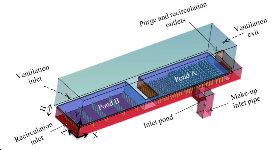
Figure 1. Schematic diagram of the large-scale fuel pond. 141
7
2
Large-Scale Cooling Pond under investigation
143Figure 1 shows a schematic diagram of the large-scale cooling ponds in a three-dimensional 144
view. The pond are characterised by large dimensions of 160m x 25m x 8m and the water 145
surface area is about 3500 m2. The whole installation consists of three different ponds. The
146
entire facility includes three different ponds. Pond A and Pond B store the heating sources 147
while the inlet pond supplies make-up. Heat removal takes place via three mechanisms: 148
ventilation, make-up water and water recirculation as illustrated in Figure 2. When the heat is 149
released from the heat sources, the water temperature starts to increase as does the heat transfer 150
from the water surface to the ambient air. The heat transfer from the water surface takes place 151
via three heat transfer modes: evaporation, convection, and radiation. The ventilation system 152
is used to replace the warm air within the building with relatively cooler air. The major heat 153
loss from the water surface is due to the evaporative component; however, this is associated 154
with the loss of pond water, which may lead to a significant drop in the water level in the long 155
term. For this reason, make-up water can be supplied to the pond to prevent the potential risk 156
of uncovering the heat sources. Furthermore, make-up water can be used for purging the pond 157
water as it has been demineralised before reaching the pond. The temperature of the make-up 158
water is mostly determined by the outside temperature. 159
Recirculation can be used on occasions when cooling by ventilation and make-up water is not 160
sufficient to control the pond temperature. Cooling via recirculation is achieved by feeding 161
some of the pond water through a cooling tower which then re-enters the pond a few degrees 162
cooler. However, cooling is not the only function of recirculation. It also helps to reduce 163
unfavourable thermal stress in the pond’s concrete walls which may otherwise lead to cracks 164
and the leakage of contaminated water. This is achieved by maintaining the water temperature 165
as uniformly distributed as possible, preventing excessive cracking in the pond walls. 166
Also, due to the long storage time of the heat load under water, a caustic dosing is injected to 167
protect the fuel cladding from any potential corrosion as well as to assist with the removal of 168
colour and turbidity present in the cooling water. In addition, the operational experience 169
showed that such chemical could help to reduce cracks in the concrete walls. In such situation, 170
recirculation of the pond water is required to improve the dispersion of the caustic dosing by 171
recirculating the pond water at various locations across the pond. 172
8 174
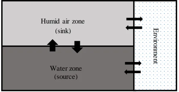
Figure 2. Description of the processes taking place within the pond installation. 175
176
177
Figure 3. Zones used in the Z-D model. 178
179
3
Z-D Model
180While developing the Z-D model for the cooling ponds, the whole pond installation is divided 181
into two nodes: the humid air zone and water zone as shown in Figure 3. These zones can be 182
described as a source and a sink, where the water zone acts as the source of water vapour and 183
Heat transfer through the wall
Hall humid air (𝑇ℎ , 𝑅𝐻)
∆𝑇𝑟𝑒𝑐 𝑁̇𝑣𝑒𝑛𝑡,𝑖𝑛
(𝑇𝑣𝑒𝑛𝑡,𝑖𝑛, 𝑅𝐻)
𝑁̇𝑣𝑒𝑛𝑡,𝑜𝑢𝑡
(𝑇ℎ , 𝑅𝐻)
Cooling tower
Evaporation
Convection Radiation
HR
𝑚̇𝑙
𝑚̇𝑚
𝑚̇𝑜𝑢𝑡
𝑚̇𝑟𝑒𝑐
Heat suorce T
p
E
n
v
iro
n
m
e
n
t
Humid air zone (sink)
9
heat energy and humid air zone acts as the sink. Energy and mass transfer with the environment, 184
the third zone, is also integral part of the model 185
The well-mixed approach is adopted in both zones. Since the heat sources are located at the 186
bottom of the pond, the water temperature for the bulk of the pond can be assumed to be 187
uniformly distributed due to buoyancy-induced convection. Similarly, the temperature of the 188
humid air zone can be treated a single value due to the large volume and the flow process of 189
evaporation. Experimental data from the site also support the above assumption. 190
The proposed Z-D model is based on solving conservation of mass and energy equations for 191
the water body and humid air zone above the water surface. The model treats each zone as a 192
single control volume and takes into account heat and mass transfer as well as interaction at 193
the air-water interface. The environment provides some boundary conditions such as 194
temperature and relative humidity to solve the ODEs involved water and humid air zones. 195
The forward time marching approach is adopted to solve a system of differential equations of 196
mass and energy using Euler's forward method as a discretization scheme [27]. This is an 197
explicit method where the solution of the current time step depends on information from the 198
previous step. The general form of Euler's method is shown in Eq. (1). The advantage of this 199
approach is that it does not require significant computing time or power and allows the 200
calculations to be performed using Microsoft Excel spreadsheet 201
202
𝑥𝑛+1 = 𝑥𝑛+ 𝑓(𝑡𝑛, 𝑥𝑛)∆𝑡 (1)
203
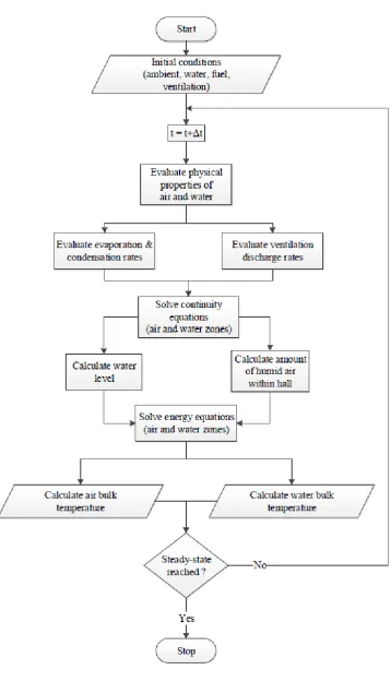
A diagrammatic representation of the Z-D model is illustrated in Figure 4. In the beginning , 204
initial values are given to start the solution. The physical properties of air and water are 205
evaluated at each time step. After that, the mass fluxes across the pond structure, evaporation 206
and condensation rates, are estimated along with the ventilation discharge rate. At this point, 207
two mass balance equations are solved in order to calculate the amounts of air and water, which 208
are needed to solve the energy equation in each zone. Finally, air and water temperatures are 209
obtained for this time step. The new temperature will be used to recalculate the physical 210
properties of air and water for the next time step. This is an iterative process that will continue 211
10 213
Figure 4. Flowchart representation of the Z-D model. 214
11
3.1 Mass Balance of the Water Zone
216
The water in the pond is evaluated at each time step, considering any change due to the supply 217
of make-up water (𝑚̇𝑚) and loss of water due to evaporation (𝑚̇𝑒𝑣), leakage (𝑚̇𝑙), and water
218
outflow (𝑚̇𝑜𝑢𝑡). Therefore, the mass balance equation for pond water can be written as follow s: 219
220
𝑚𝑝𝑛+1= 𝑚𝑝𝑛+ (𝑚̇𝑚− 𝑚̇𝑜𝑢𝑡− 𝑚̇𝑒𝑣− 𝑚̇𝑙)𝑛 ∆𝑡 (2)
221
where 𝑚𝑝 is the total mass of water within the ponds, ∆𝑡 is the time step size, and 𝑛 is the
222
number of iterations. 223
The following equation describes how the water outflow from the pond is controlled. When 224
the water loss due to evaporation and leakage is greater than the supplied make-up water, no 225
water discharge will be permitted. Similarly, in situations when the height of the water level 226
(𝐻) is lower than its designed value (𝐻𝐷), no water outflow is allowed until the water level
227
reaches this value. The following relationship explains how the outflow of water can be 228
mathematically expressed: 229
230
𝑚̇𝑜𝑢𝑡=
{
0 𝑖𝑓 (𝑚̇𝑒𝑣+ 𝑚̇𝑙) ≥ 𝑚̇𝑚
𝑚̇𝑚− 𝑚̇𝑒𝑣− 𝑚̇𝑙 𝑖𝑓 (𝑚̇𝑒𝑣+ 𝑚̇𝑙) < 𝑚̇𝑚
0 𝑖𝑓 𝐻 ≤ 𝐻𝐷
[𝜌𝑤 𝐴𝑝(𝐻 − 𝐻𝐷)
∆𝑡 ] + (𝑚̇𝑚− 𝑚̇𝑒𝑣− 𝑚̇𝑙) 𝑖𝑓 𝐻 > 𝐻𝐷
(3)
231
where 𝜌𝑤 is the water density and 𝐴𝑝 is the water surface area of the pond. The evaporation
232
rate before the pond water starts to boil can be estimated using Stefan’s law [28]. The following 233
equations show how the evaporation rate can be estimated before boiling and in the case of 234
boiling. 235
12
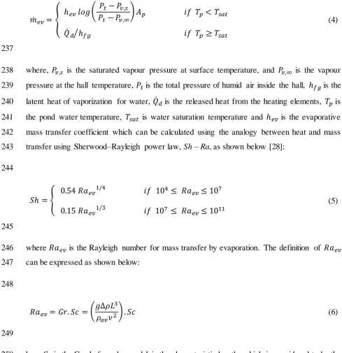
𝑚̇𝑒𝑣= {
ℎ𝑒𝑣 𝑙𝑜𝑔 ( 𝑃𝑡− 𝑃𝑣,𝑠
𝑃𝑡− 𝑃𝑣,∞) 𝐴𝑝 𝑖𝑓 𝑇𝑝< 𝑇𝑠𝑎𝑡
𝑄̇𝑑⁄ℎ𝑓𝑔 𝑖𝑓 𝑇𝑝 ≥ 𝑇𝑠𝑎𝑡
(4)
237
where, 𝑃𝑣,𝑠 is the saturated vapour pressure at surface temperature, and 𝑃𝑣,∞ is the vapour 238
pressure at the hall temperature, 𝑃𝑡 is the total pressure of humid air inside the hall, ℎ𝑓𝑔 is the
239
latent heat of vaporization for water, 𝑄̇𝑑 is the released heat from the heating elements, 𝑇𝑝 is 240
the pond water temperature, 𝑇𝑠𝑎𝑡 is water saturation temperature and ℎ𝑒𝑣 is the evaporative
241
mass transfer coefficient which can be calculated using the analogy between heat and mass 242
transfer using Sherwood–Rayleigh power law, Sh – Ra,as shown below [28]: 243
244
𝑆ℎ = {
0.54 𝑅𝑎𝑒𝑣1/4 𝑖𝑓 104≤ 𝑅𝑎𝑒𝑣≤ 107
0.15 𝑅𝑎𝑒𝑣1/3 𝑖𝑓 107 ≤ 𝑅𝑎𝑒𝑣≤ 1011
(5)
245
where 𝑅𝑎𝑒𝑣 is the Rayleigh number for mass transfer by evaporation. The definition of 𝑅𝑎𝑒𝑣
246
can be expressed as shown below: 247
248
𝑅𝑎𝑒𝑣= 𝐺𝑟. 𝑆𝑐 = (𝑔∆𝜌𝐿
3
𝜌𝑎𝑣𝜈2) . 𝑆𝑐 (6)
249
here 𝐺𝑟 is the Grashof number and 𝐿 is the characteristic length, which is considered to be the 250
area of the water surface over its perimeter. 251
252
3.2 Pond Water Elevation
253
The pond water level is calculated by knowing the water volume and the surface area of the 254
pond water. When the water level drops to a value less than the rack height (𝐻𝑅) shown in 255
13
rack assemblies (𝐴𝑅). The water level at every time step is updated according to the mass of
257
water available in the pond, as shown in the following equation: 258
259
𝐻 =
{
[(𝑚𝑝
𝜌𝑤
− 𝐴𝑅𝐻𝑅) 𝐴⁄ 𝑝] + 𝐻𝑅 𝑖𝑓 𝐻 ≥ 𝐻𝑅
(𝑚𝑝 𝜌𝑤
) /𝐴𝑅 𝑖𝑓 𝐻 < 𝐻𝑅
(7)
260
3.3 Mass Balance of the Humid Air Zone
261
Humid air is considered as a mixture of dry air and water vapour. Both dry air and water vapour 262
at low partial pressure can be treated as a perfect gas. When dealing with humid air, it is more 263
convenient that the mass of the moist air to be expressed in mole basis for the dry air and vapour 264
separately. 265
In order to evaluate the amount of dry air (𝑁𝑎) and vapour (𝑁𝑣) inside the pond hall, the mass
266
balance equation across the hall is applied as shown in Equations (8) and (9). This mass balance 267
takes into account the ventilation inlet (𝑁̇𝑣𝑒𝑛𝑡,𝑖𝑛) and discharge (𝑁̇𝑣𝑒𝑛𝑡,𝑜𝑢𝑡) flow rates as well
268
as evaporation and condensation (𝑚̇𝑐𝑜𝑛) rates. 269
270
𝑁𝑎𝑛+1= 𝑁𝑎𝑛+ (𝑦𝑣𝑒𝑛𝑡 ,𝑖𝑛𝑎 𝑁̇𝑣𝑒𝑛𝑡,𝑖𝑛− 𝑦ℎ𝑎 𝑁̇𝑣𝑒𝑛𝑡,𝑜𝑢𝑡) 𝑛
∆𝑡 (8)
271
𝑁𝑣𝑛+1= 𝑁
𝑣𝑛+ (𝑁̇𝑣𝑒𝑛𝑡,𝑖𝑛− 𝑦ℎ𝑣 𝑁̇𝑣𝑒𝑛𝑡,𝑜𝑢𝑡+
𝑚̇𝑒𝑣
𝑀𝑣 −
𝑚̇𝑐𝑜𝑛
𝑀𝑣 )
𝑛
∆𝑡 (9)
272
where 𝑦𝑣𝑒𝑛𝑡 ,𝑖𝑛𝑎 is the molar fractions of dry air of the incoming ventilation air and 𝑦ℎ𝑎 and 𝑦ℎ𝑣
273
are the molar fractions of dry air and water vapour respectively, which can be found from: 274
275
𝑦ℎ𝑎 =𝑁𝑎
14 276
𝑦ℎ𝑣 = 𝑁𝑣 𝑁ℎ
(11) 277
𝑁ℎ= 𝑁𝑎+ 𝑁𝑣 (12)
278
Here 𝑁ℎ is the total molar mass of the humid air inside the pond hall. The flow rate of the
279
ventilation inlet is an initial input condition, where the differential pressures drive the 280
ventilation discharge and can be computed from: 281
282
𝑁̇𝑣𝑒𝑛𝑡,𝑜𝑢𝑡= 𝜌∞ 𝑀𝑣𝐴𝑑𝑢𝑐𝑡√2(𝑃𝑡− 𝑃𝑎𝑡𝑚) 𝜌∞
(13) 283
where 𝜌∞ is the density of the humid air inside the pond hall, 𝑀𝑣 is the molecular weight of
284
water vapour, 𝐴𝑑𝑢𝑐𝑡 is the cross-sectional area of the ventilation discharge duct, 𝑃𝑎𝑡𝑚 is the
285
outside atmospheric pressure 𝑃𝑡 is the total pressure of humid air inside the pond hall and can 286
be evaluated as follow: 287
288
𝑃𝑡= (
𝑇ℎ𝑅𝑜
𝑉ℎ
) 𝑁ℎ (14)
289
The estimation of the condensation rate is similar to the calculation of the evaporation rate: 290
291
𝑚̇𝑐𝑜𝑛= ℎ𝑐𝑜𝑛(𝜌𝑣,∞− 𝜌𝑣,𝑤𝑎𝑙𝑙) 𝐴ℎ (15)
292
where, 𝜌𝑣,𝑤𝑎𝑙𝑙 is the saturated vapour density at wall temperature, 𝐴ℎ is surface area of the 293
inner walls of the pond hall and ℎ𝑐𝑜𝑛 is the condensation mass transfer coefficient which can 294
15
296
𝑆ℎ = 0.10 𝑅𝑎1/3 (16)
297
To examine the coefficient 0.10 in Eq. (16), we have run several calculations considering 298
different values for this coefficient ranging from 0.05 to 0.2. It was found that the maximum 299
effect of this coefficient on the final result for the water temperature is relatively low, less than 300
1.5%. 301
3.4 Energy Balance of the Water Zone
302
The energy contained in the water body is integrated over time taking into account the heat 303
realised from the heat sources, the heat flux from the water surface and the energy associated 304
with the water inlets and outlets: 305
306
𝑇𝑝𝑛+1
= 𝑇𝑝𝑛+ (𝑄̇
𝑑+ 𝑚̇𝑚𝐶𝑤𝑇𝑚− 𝑚̇𝑜𝑢𝑡𝐶𝑤𝑇𝑝− 𝑚̇𝑒𝑣𝐶𝑤𝑇𝑝− 𝑚̇𝑟𝑒𝑐𝐶𝑤∆𝑇𝑟𝑒𝑐− 𝑄̇𝑠)
𝑛 ∆𝑡
𝑚𝑝𝐶𝑤
(17)
307
where 𝐶𝑤 is the specific heat of water, 𝑇𝑚 is the temperature of the make-up water, 𝑚̇𝑟𝑒𝑐 is the
308
recirculation flow rate, ∆𝑇𝑟𝑒𝑐 is the temperature drop in the cooling tower which is controlled
309
by the wet bulb temperature of the outdoor air (𝑇𝑤𝑏) and the cooling tower efficiency and can 310
be expressed as: 311
312
ζ = ∆𝑇𝑟𝑒𝑐
𝑇𝑝− 𝑇𝑤𝑏 (18)
313
and 𝑄̇𝑠 is the total heat transfer at the air-water interface which can be estimated as shown
314
below: 315
16
𝑄̇𝑠= 𝑄̇𝑒𝑣+ 𝑄̇𝑟+ 𝑄̇𝑐 (19)
317
where 𝑄̇𝑒𝑣 is the evaporative heat transfer, 𝑄̇𝑟 is the radiative heat transfer, and 𝑄̇𝑐 is the 318
convective heat transfer. These three heat transfer modes can be evaluated from the following 319
expressions: 320
321
𝑄̇𝑒𝑣= 𝑚̇𝑒𝑣ℎ𝑓𝑔 (20)
322
𝑄̇𝑟= 𝐴𝑝𝜀 𝜎(𝑇𝑝4− 𝑇𝑤𝑎𝑙𝑙4 ) (21)
323
𝑄̇𝑐= 𝐴𝑝ℎ𝑐(𝑇𝑝− 𝑇ℎ) (22)
324
Here 𝜀 is emissivity, 𝜎 is the Stefan Boltzmann constant, 𝑇𝑤𝑎𝑙𝑙 is the wall inner surface
325
temperature of the hall, ℎ𝑐 is the convection heat transfer coefficient at the water surface which 326
may be evaluated by using the Nusselt–Rayleigh power law, 𝑁𝑢 − 𝑅𝑎, as shown below: 327
328
𝑁𝑢 = {
0.54 𝑅𝑎1/4 𝑖𝑓 104 ≤ 𝑅𝑎 ≤ 107
0.15 𝑅𝑎1/3 𝑖𝑓 107 ≤ 𝑅𝑎 ≤ 1011
(23)
329
3.5 Energy Balance of the Humid Air Zone
330
The heat loss from the water surface is gained by the ventilated air, which results in an increase 331
in air temperature. To calculate the air temperature inside the pond hall, the energy balance is 332
performed across the hall as shown below: 333
334
𝑇ℎ𝑛+1= 𝑇ℎ𝑛+ [𝑚̇𝑒𝑣ℎ 𝑣(𝑇𝑝) + 𝑄̇𝑐+ 𝑄̇𝑟− 𝑄̇𝑤𝑎𝑙𝑙− 𝑚̇𝑐𝑜𝑛ℎ𝑓𝑔+ 𝑄̇𝑣𝑒𝑛𝑡,𝑖𝑛−
𝑄̇𝑣𝑒𝑛𝑡,𝑜𝑢𝑡]
𝑛 ∆𝑡
[𝑁𝑎𝑀𝑎𝐶𝑝,𝑎+𝑁𝑣𝑀𝑣𝐶𝑝,𝑣]
17 335
where ℎ𝑣(𝑇) is the specific enthalpy of water vapour at a given temperature and can be
336
calculated using the shown below [29]. However, this relationship is valid only for low values 337
of pressure. 338
339
ℎ𝑣(𝑇) = 2500 + 1.82 (𝑇 − 273) (25)
340
In order to obtain the heat energy associated with the incoming ventilated humid air (𝑄̇𝑣𝑒𝑛𝑡,𝑖𝑛)
341
and the discharged humid air by ventilation (𝑄̇𝑣𝑒𝑛𝑡,𝑜𝑢𝑡), the following relationships are used:
342 343
𝑄̇𝑣𝑒𝑛𝑡,𝑖𝑛= 𝑦𝑣𝑒𝑛𝑡 ,𝑖𝑛𝑎 𝑁̇𝑣𝑒𝑛𝑡,𝑖𝑛𝐶𝑝,𝑎𝑇𝑣𝑒𝑛𝑡,𝑖𝑛+ 𝑦𝑣𝑒𝑛𝑡 ,𝑖𝑛𝑣 𝑁̇𝑣𝑒𝑛𝑡,𝑖𝑛ℎ 𝑣(𝑇𝑣𝑒𝑛𝑡,𝑖𝑛) (26)
344
𝑄̇𝑣𝑒𝑛𝑡,𝑜𝑢𝑡= 𝑦ℎ𝑎 𝑁̇𝑣𝑒𝑛𝑡,𝑜𝑢𝑡𝐶𝑝,𝑎𝑇ℎ+ 𝑦ℎ𝑣 𝑁̇𝑣𝑒𝑛𝑡,𝑜𝑢𝑡ℎ 𝑣(𝑇ℎ) (27) 345
Here, 𝑦𝑣𝑒𝑛𝑡,𝑖𝑛𝑎 and 𝑦𝑣𝑒𝑛𝑡 ,𝑖𝑛𝑣 are the molar fractions of the ventilation inlet dry air and vapour 346
respectively, 𝐶𝑝,𝑎 is the specific heat of the dry air, and 𝑇𝑣𝑒𝑛𝑡,𝑖𝑛 is the ventilation inlet 347
temperature which is assumed to be the same as the outside temperature. The heat transfer 348
through the walls of the pond hall (𝑄̇𝑤𝑎𝑙𝑙) is computed according to:
349 350
𝑄̇𝑤𝑎𝑙𝑙= ℎ𝑖𝑛( 𝑇ℎ− 𝑇𝑤𝑎𝑙𝑙) 𝐴ℎ (28)
351
In order to determine 𝑇𝑤𝑎𝑙𝑙, an energy balance is performed across the walls of the pond hall
352
where the wall thickness (𝑥) is divided to uniform increments of 𝑑𝑥. The energy equations for 353
the interior and surface layers can be written as follow: 354
18
𝑇𝑖𝑛+1= 𝑇𝑖𝑛+ 𝑘
𝑑𝑥 𝐶𝑤𝑎𝑙𝑙𝜌𝑤𝑎𝑙𝑙
(𝑇𝑖 −1− 𝑇𝑖
𝑑𝑥 −
𝑇𝑖− 𝑇𝑖+1
𝑑𝑥 )
𝑛
∆𝑡 (29)
356
𝑇𝑖𝑛+1= 𝑇𝑖𝑛+ 𝑘
𝑑𝑥 𝐶𝑤𝑎𝑙𝑙𝜌𝑤𝑎𝑙𝑙(
𝑇𝑤𝑎𝑙𝑙− 𝑇𝑖
𝑑𝑥/2 −
𝑇𝑖− 𝑇𝑖+1
𝑑𝑥 )
𝑛
∆𝑡 (30)
357
where 𝑖 is the index of the wall layers, 𝐶𝑤𝑎𝑙𝑙 is the specific heat of the walls material, 𝜌𝑤𝑎𝑙𝑙 is 358
the density of the walls material, and 𝑘 is the thermal conductivity of the walls material. The 359
inner and outer surface temperatures can be calculated considering the heat balance across this 360
surface as shown below, respectively: 361
362
𝑄̇𝑟+ (𝑇ℎ− 𝑇𝑤𝑎𝑙𝑙)𝐴ℎℎ𝑖𝑛=
𝑇𝑤𝑎𝑙𝑙− 𝑇𝑖
𝑑𝑥/2 𝐴ℎ𝑘 (31)
363
(𝑇𝑜𝑢𝑡 − 𝑇𝑒𝑛𝑣)𝐴ℎℎ0𝑢𝑡=
𝑇𝑖 − 𝑇𝑜𝑢𝑡
𝑑𝑥/2 𝐴ℎ𝑘 (32)
364
where 𝑇𝑒𝑛𝑣 is the outside environment temperature ℎ𝑖𝑛 is the convective heat transfer 365
coefficient for the inner surface of the pond hall and ℎ0𝑢𝑡 is the outer surface heat transfer
366
coefficient and was considered to be constant (4 W/m2 K). Finally, under the normal
367
operational conditions, the solution is considered to be converged when the relative difference 368
between the current iteration and the previous iteration is less than 0.01%. The convergence 369
criterion is expressed as shown below: 370
371
Convergence criterion =|𝑇𝑝
𝑛+1− 𝑇 𝑝𝑛|
𝑇𝑝𝑛
× 100 (33)
372
However, this convergence criterion cannot be applied when the pond is suffering from loss of 373
19
saturation is reached. During this time, the water level may drop until the pond dries out unless 375
sufficient make-up water is provided to compensate for the evaporated water. 376
377
The heat loss from the pond water to the concrete wall is not considered in this study as it 378
makes only a tiny contribution to the total heat loss from the pond's structure. This is because 379
the ponds are surrounded by a very thick concrete layer at the sides and floor. 380
As mentioned before, the calculations were performed using the explicit Euler’s method, which 381
is known to be conditionally stable, hence, a stability analysis is required [30]. Investigation of 382
the numerical behaviour of the model shows that the stability of the model is more dominated 383
by the stability of the differential equations rather than the used method. The highest instability 384
was observed in the mass balance equation for the humid air zone. This is due to the pressure 385
fluctuation, which is mostly controlled by the ventilation discharge. Therefore, a stability 386
analysis is conducted on the mass balance equation for the humid air zone. However, to perform 387
such analysis, the nonlinear equations have to be linearized. The linearization of the ODE for 388
the mass balance of the humid air zone was achieved using Taylor series. Then, a systematic 389
stability analysis was accomplished as follows: 390
• Construct the finite difference equation (FDE) for the model ODE, 𝑦́ + 𝜙𝑦 = 0
391
• Determine the amplification factor, G, of the FDE. 392
• Determine the conditions to ensure that |G| < 1. 393
By applying the above-mentioned practice, an estimation of the limit of the stable time step 394
can be expressed as: 395
∆𝑡 < 2
𝜃 (34)
396
where 𝜃 is equivalent to: 397
398
𝜃 =𝐴𝑑𝑢𝑐𝑡𝑅𝑜𝑇ℎ
2𝑉ℎ √
2𝜌∞
(𝑇ℎ𝑅𝑜
𝑉ℎ ) 𝑁ℎ
𝑛− 𝑃 𝑎𝑡𝑚
(35)
20
Note that 𝜃 changes as 𝑁ℎ𝑛 changes. Thus, the stable step size changes as the solution advances. 400
However, keeping the time step within the criterion shown in Eq. (34) not only ensures 401
stability, but it also ensures that the results are not very sensitive to the time step. According to 402
this criterion, the used time step in all the cases presented in this study is 5 sec. 403
4
Z-D Model Validation
404The Z-D thermal model of the cooling pond is validated against available data for two different 405
cooling ponds as shown below: 406
1. Maine Yankee spent fuel pool, Wiscasset, USA [18] 407
2. The large-scale cooling pond 408
4.1 Validation with Maine Yankee Pool Data
409
The Maine Yankee spent fuel pool is a relatively small cooling pond located at the reactor site, 410
with dimensions of 12.6 m long, 11.3 m wide and 11.1 m deep. Carlos et al. [18] used TRACE 411
best estimate code to analyse the response of the cooling pond in different scenarios. During 412
their calculations, no heat loss was considered at the free water surface except when the water 413
has reached its saturation temperature (100 oC) with the initiation of boiling. However, this
414
assumption does not have a significant effect on the results, as the proportion of heat loss from 415
the water surface before boiling is not significant compared to the heat loss by the supplied 416
water. This is owing to the small surface area at the air-water interface. 417
The Z-D model is used to perform calculations on the Maine Yankee spent fuel pool, Wiscasset, 418
USA [18] and the results obtained are compared against the published data for this pool. These 419
calculations are developed for three cases: (a) steady-state, (b) licensing, and (c) accident 420
scenarios. 421
In the paper reported by Carlos et al. [18], the temperature data were available for the steady-422
state case in the form of actual temperature measurements collected from the Maine Yankee 423
spent fuel pool. For the licensing case, the temperature data were calculated by GFLOW 424
software [31], while the TRACE best estimate code was used for the pool temperature under 425
21 (a) - (b) Steady-state and Licensing Cases 427
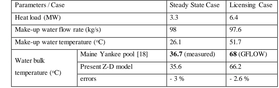
The input parameters used in the calculations of the steady-state and licensing cases are 428
summarised in Table 1. In the same table, the outcomes from the validation exercise our Z-D 429
model are presented. The heat load in the licensing case corresponds to the maximum expected 430
heat generation from the fuel elements. 431
The results predicted by the Z-D model are in good agreement with the available data for the 432
Maine Yankee spent fuel pool as can be seen in Table 1. However, the Z-D model 433
underestimates the pond water temperature by 3 % and 2.6 % for steady-state and licensing 434
cases respectively. When all of the heat transfer modes from the water surface are deactivated 435
in the Z-D model calculations, except for boiling, the underestimation errors of the water 436
temperature decreased to 1.9 % and 0.9 % for the steady-state and licensing cases respectively. 437
This implies that the heat loss from the water surface before boiling is relatively less significant, 438
as mentioned before. 439
440
Table 1. Input data and comparison between values predicted by the Z-D model and data for 441
the Maine Yankee pool [18]. 442
Parameters / Case Steady State Case Licensing Case
Heat load (MW) 3.3 6.4
Make-up water flow rate (kg/s) 98 97.6
Make-up water temperature (oC) 26.1 51.7
Water bulk temperature (oC)
Maine Yankee pool [18] 36.7 (measured) 68 (GFLOW)
Present Z-D model 35.6 66.2
errors - 3 % - 2.6 %
443
(c) Accident Case 444
The outcomes from the licensing case were used as the input data for the accident scenario 445
except for the initial water level which is considered to have a value of 4.56 m as measured 446
from the bottom of the pond. In the TRACE simulation for the accident case, it was assumed 447
that the pumps which supply the pond with the cooling and make-up water, have stopped 448
22
means of boiling. Therefore, in the Z-D model calculations, the heat transfer modes from the 450
water surface were deactivated and the only heat transfer permitted is due to boiling. 451
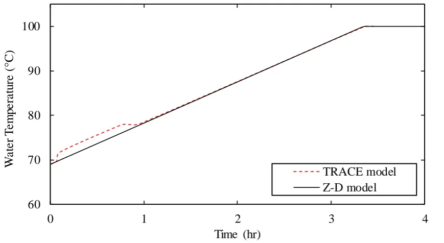
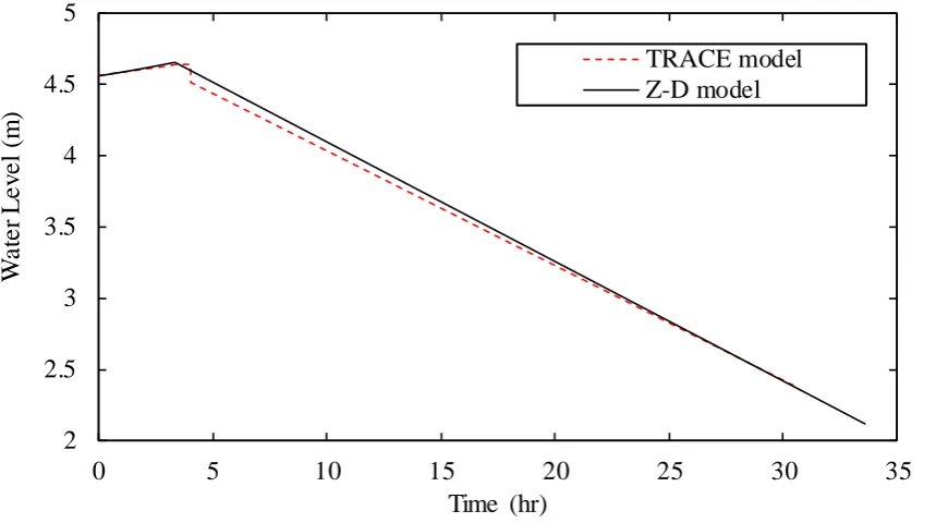
Figures 5 and 6 show comparisons between the results predicted by the Z-D model and the 452
TRACE data for the accident scenario in terms of water temperature and drop of pond water 453
level respectively. In Figure 5, for up to one hour the same linear trend is observed, but a clear 454
shift of 1.8 oC is recorded, the reason for which is not obvious from the original paper [18].
455
Figure 6 shows a sudden drop in water level over a very short time (something similar to 456
purging), but the reason for such behaviour was also not explained. These behaviours may be 457
due to assumptions made which are unknown to us. In general, good agreement can be observed 458
between the Z-D model and the TRACE best estimate code. 459
460
Figure 5. Comparison of water temperature for the accident case that obtained by the proposed 461
Z-D model and Maine Yankee pool [18]. 462
463
60 70 80 90 100
0 1 2 3 4
W
a
te
r
T
e
m
p
e
ra
tu
re
(
°C
)
Time (hr)
23
464
Figure 6. Comparison of water level for the accident case that obtained by the proposed Z-D 465
model and Maine Yankee pool [18]. 466
4.2 Validation with Large-Scale Cooling Pond Data
467
The validation exercise is further extended to consider a large-scale cooling pond to examine 468
the effect of pond size on the Z-D model’s prediction. The total heat realised from the heat 469
sources is about 340 kW. 470
The validation is performed for three different operational configurations and the input 471
parameters used during these calculations are summarised in 472
473 474 475
Table 2. Comparisons between the measured data and the results predicted by the Z-D model 476
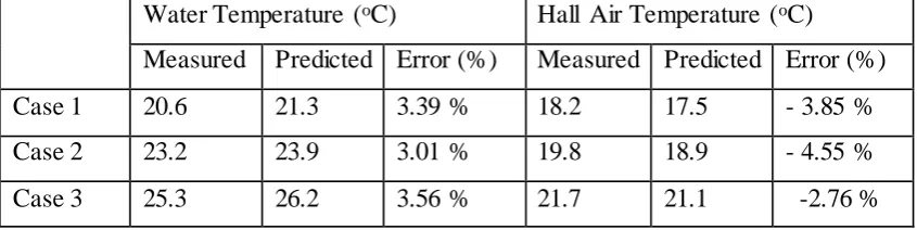
are presented in tabular form as shown in Table 3. It can be seen from the comparisons that the 477
Z-D model has predicted the water temperature as well as the hall air temperature within a good 478
level of accuracy. However, the Z-D model has slightly overestimated the water temperature. 479
The maximum observed error in the predictions of water temperature is 3.56 %, where the 480
maximum recorded error in the hall air temperature is - 4.55 %. 481
482
2 2.5 3 3.5 4 4.5 5
0 5 10 15 20 25 30 35
W
a
te
r
L
e
v
e
l
(m
)
Time (hr)
24 483
484 485
Table 2. Input parameters used in validation with the large-scale cooling pond data. 486
Parameters Case 1 Case 2 Case 3
Initial water level (m) 8 8 8
Water surface area (m2) 3,500 3,500 3,500
Water zone volume (m3) 21,900 21,900 21,900
Humid air zone volume (m3) 129,600 129,600 129,600
Heat transfer area of humid air zone (m2) 15,120 15,120 15,120
Heat load (kW) 340 340 340
Outside environment temperature (oC) 11 14 19
Recirculation flow rate (kg/s) 4.57 4.63 4.05 Temperature drop in cooling tower (oC) 0 0 3
Make-up rate (kg/s) 3.47 3.62 3.84
Make-up temperature (oC) 10 14 20
Ventilation inlet rate (m3/s) 12 12 12
487
Table 3. Comparison between measured and predicted results for the large-scale cooling 488
ponds data. 489
Water Temperature (oC) Hall Air Temperature (oC)
Measured Predicted Error (%) Measured Predicted Error (%)
Case 1 20.6 21.3 3.39 % 18.2 17.5 - 3.85 %
Case 2 23.2 23.9 3.01 % 19.8 18.9 - 4.55 %
Case 3 25.3 26.2 3.56 % 21.7 21.1 -2.76 %
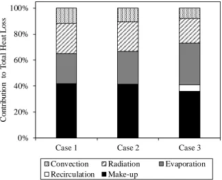
490
The percentage contribution of each heat removal mode to the total heat loss is shown in Figure 491
7 for the three validation cases. These contributions are evaluated when the steady state is 492
reached. From the results shown in this figure, it is obvious that the heat loss from the water 493
25
under different configurations, these ratios can vary significantly. For an instant, when the 495
make-up water or recirculation flow rates are high, this will lead to much higher contributions 496
of these heat removal modes over the surface heat loss. 497
498
499
Figure 7. Contribution percentage of different heat removal modes for validation case 1, case 500
2, and case 3. 501
5
Analysis of Pond Behaviour
502After confirming the reliability of the Z-D model, it was used to study the thermal behaviour 503
of the large-scale cooling pond, and in addition, to assess the suitability of using particular 504
assumptions in certain cases. From the point of view safety and economics, it is essential to 505
analyse the performance of the pond under normal operating conditions as well as accident 506
scenarios. 507
5.1 Normal Operating Conditions
508
The calculations in this section are performed considering that the pond is loaded with the 509
maximum possible heat load and all of the cooling systems are in place and under control. The 510
maximum heat load is 11 MW, which corresponds to the maximum expected amount of heat 511
sources to be stored and is assumed to be uniformly distributed throughout the pond. The input 512
parameters used in this calculation are listed in Table 4. 513
0% 20% 40% 60% 80% 100%
Case 1 Case 2 Case 3
Co
n
tri
b
u
ti
o
n
to
T
o
ta
l
H
e
a
t
L
o
ss
26 514
Table 4. Configurations used in the case of normal operating conditions. 515
Parameters
Initial water level (m) 8
Water surface area (m2) 3500
Water zone volume (m3) 21900
Humid air zone volume (m3) 129600
Heat transfer area of humid air zone (m2) 15120
Heat load (MW) 11
Outside environment temperature (oC) 14
Recirculation flow rate (kg/s) 115.74 Cooling tower efficiency (%) 60
Make-up rate (kg/s) 13.9
Make-up temperature (oC) 14
Ventilation inlet rate (m3/s) 12
516
The results for the normal operations case are presented in Figure 8 in terms of water and hall 517
temperatures. As shown in this figure, at the beginning of the calculations the water and air 518
temperatures have the same value of 14 oC. As time progresses, both water and air temperatures
519
increase until the steady state is reached at values of 41.5 oC for the water and about 31.3 oC
520
27 522
Figure 8. Water and air temperatures under normal operating conditions for the large-scale 523
cooling pond at a heat load of 11 MW. 524
525
The generated heat is removed via different modes as shown in Figure 9. Furthermore, this 526
figure illustrates the contribution of the heat removal component to the total heat removed from 527
the water body. The generated heat being removed by the recirculation is dominated the cooling 528
process with a percentage of 75 % of the total heat loss. It appears that the heat loss from the 529
water surface represents a relatively small proportion (8%) of the total heat loss, but it cannot 530
be ignored. However, the scenario can be different for lower heat loads as in the cases presented 531
in the validation section for the large-scale cooling ponds as shown in Figure 7. 532
533
10 15 20 25 30 35 40 45 50
0 2 4 6 8 10 12 14
T
e
m
p
e
ra
tu
re
(
o C)
Time (day)
28 534
Figure 9. The contribution of different heat removal modes under normal operating conditions 535
for the large-scale cooling pond. 536
537
5.2 Loss of Cooling Scenario
538
In this section, we assume that a power blackout and total loss of the cooling systems occurs 539
with no accident mitigation measures are in place. The calculations are conducted for the large-540
scale cooling pond taking the outcomes from the previous case of normal operating conditions 541
as initial values. Moreover, the calculations are performed for two different conditions at the 542
water surface. The first condition ignores the heat loss from the water surface except for the 543
boiling heat transfer, which is represented in the graphs by “Heat off”. The second condition 544
takes into account all the heat transfer modes at the water surface, which is represented in the 545
graphs by “Heat on”. 546
As can be seen from Figures 10 and 11 that at the “Heat off” condition, the water temperature 547
reaches boiling after 5.6 days. Meanwhile, the water level reaches its highest value due to a 548
decrease in water density and then starts to drop until the fuel assemblies begin to be uncovered 549
at approximately day 37. At this point, make-up water is injected to recover the pond water 550
temperature and level. To achieve this, 2.5 days is required to recover the water level and 18 551
days for the water temperature to drop to about 50.7 °C. 552
77%
15%
5% 2%
1% 0%
20% 40% 60% 80% 100%
Recirculation Make-up Evaporation Radiation Convection
H
e
a
t
L
o
ss
(M
W
29
For the “Heat on” condition, the estimation of the time required for the fuel assembly to start 553
to be uncovered is the same as in the “Heat on” case. On the other hand, water reaches its 554
saturation temperature 2 days earlier than the predicted time in the “Heat on” case. However, 555
these differences, in the presented case, are still within a good level and provide a conservative 556
treatment for the accident scenario. For different conditions, the assumption that the heat loss 557
from the water surface can be neglected may not be appropriate. For example, Figure 12 shows 558
the effect of heat load on the validity of this assumption for different heat loads. 559
560
561
Figure 10. Water temperature during the loss of cooling scenario and after injection of make-562
up water for the large-scale cooling pond. 563
564
40 50 60 70 80 90 100
0 5 10 15 20 25 30 35 40 45 50 55
W
a
te
r
T
e
m
p
e
ra
tu
re
(
°C
)
Time (day)
Heat off Heat on
30 565
Figure 11. Water level during the loss of cooling scenario and after injection of make-up water 566
for the large-scale cooling pond. 567
In Figure 12, for the “Heat off” situation, the sensible heating is faster for the high heat load 568
and once the temperature reaches the boiling point, for both heat loads, the curves become 569
parallel to X-axis. It can also be seen that adopting such “Heat off” assumption can significant ly 570
overpredicts the water temperature especially for low heat load values. In Figure 12, the 571
difference between the predictions of water temperature using both assumptions is around 48% 572
for a heat load of 0.5 MW, whereas only 18% is observed for the heat load of 2 MW. This 573
implies that the over-prediction is higher for the low heat load. This is due, as discussed before, 574
to the large exposed area of the water surface to the ambient air, which increases the surface 575
heat loss. Hence, such an assumption should be carefully considered while performing the 576
analysis of accident scenarios for large-scale cooling ponds. 577
578
0 1 2 3 4 5 6 7 8 9
0 5 10 15 20 25 30 35 40 45 50 55
W
a
te
r
L
e
v
e
l
(m
)
Time (day)
Heat off Heat on Injection of
Make-up water level of heat
31
579
Figure 12. Water temperature under different heat loads for the large-scale cooling pond. 580
581
5.3 Impact of Weather Conditions
582
The outside weather conditions are represented in the Z-D model in terms of outside air 583
temperature and relative humidity. Changes in these conditions may have an effect on the 584
cooling performance of the spent pond. To examine the potential effects, we have conducted a 585
sensitivity study by varying the outside air temperature and relative humidity. As can be seen 586
in Figure 13, the outside air temperature has a significant effect on the water temperature. 587
Increasing the outside air temperature by about 10 °C results in an increase in the water 588
temperature by approximately 9 °C. This is because of the make-up water and ventilation air 589
temperatures are mostly determined by the outside temperature. Also, the temperature drop in 590
the cooling tower, as shown in Figure 2, is affected by the conditions outside. 591
On the other hand, the relative humidity of the outside air does not have a considerable effect, 592
as shown in Figure 14. This may be because of the air change per hour (ACH) for the pond hall 593
is very low for this type of applications, at about 0.333 per hr. Meanwhile, the amount of water 594
vapour emerging from the water surface due to evaporation is high enough to rapidly increase 595
the relative humidity of the moist air within the pond hall. 596
40 50 60 70 80 90 100
0 10 20 30 40 50 60 70 80 90 100 110 120 130
W
a
te
r
T
e
m
p
e
ra
tu
re
(
°C
)
Time (day)
32 597
Figure 13. Effect of outside ambient air temperature on water temperature assuming 0% 598
relative humidity. 599
600 601
602
Figure 14. Effect of the outside relative humidity on water temperature assuming an air 603
temperature of 25 °C. 604
10 20 30 40 50 60
0 2 4 6 8 10 12 14 16 18 20
W
a
te
r
T
e
m
p
e
ra
tu
re
(
°C)
Time (day)
Outside temperature =25 °C Outside temperature =15 °C Outside temperature =5 °C
10 20 30 40 50 60
0 2 4 6 8 10 12 14
W
a
te
r
T
e
m
p
e
ra
tu
re
(
°C)
Time (day)
33
6
Conclusion
605
A Z-D model has been developed for large-scale cooling ponds. This model was validated 606
against data reported in the literature for the Maine Yankee spent fuel cooling pond. Also, 607
another validation exercise was performed to examine the applicability of the Z-D model to 608
predict the water temperature for the large-scale cooling pond. However, this validation was 609
limited to low water temperatures where validation with higher water temperatures (near 100 610
°C) has not been conducted due to the limited data available for the large-scale cooling ponds 611
and the difficulty of producing such data. It can be seen from the validation exercises that the 612
Z-D thermal model is able to predict the thermal behaviour of the cooling ponds under the 613
considered operational scenarios and with various pond sizes. 614
A number of parametric studies were performed in different situations. The first study 615
concerned the performance of the pond under normal operating conditions where the pond 616
water and air temperatures are evaluated. In the same study, the proportions of heat removal 617
components were quantified. Furthermore, a loss of cooling analysis was conducted under two 618
conditions; one without surface heat transfer and another with heat transfer. It was found that 619
the assumption leading to ignoring the heat loss from the water surface is not always a good 620
choice. 621
The last study was performed to examine the sensitivity of the pond water temperature to 622
variation in outside weather conditions. The outcomes reveal that water temperature is rather 623
insensitive to the outside relative humidity under the given scenario and the assumption of 624
constant efficiency of the cooling tower, which limits the effect of the relative humidity on the 625
cooling tower performance. On the other hand, relatively high sensitivity was observed to 626
variations in outside temperature. However, further sensitivity studies are needed to determine 627
the effect of the input parameters on the Z-D model’s predictions. These studies can be 628
conducted using an appropriate statistical method in combination with the D model. The Z-629
D model will allow many studies to be performed within a reasonable time. In order to improve 630
the Z-D model, a full description of the cooling tower process need to be included. 631
References
632[1] B. Zohuri and N. Fathi, Thermal-hydraulic analysis of nuclear reactors. Springer, 633
2015. 634
[2] W. Kuo, G. Yun, and Z. He-yi, "Spent fuel pool transient analysis under accident case 635
and the flow establishment process of passive cooling system," in Information Systems
34
for Crisis Response and Management (ISCRAM), 2011 International Conference on, 637
2011, pp. 482-491: IEEE. 638
[3] UK Government. (September 15, 2016). Government confirms Hinkley Point C project
639
following new agreement in principle with EDF. Accessed 10 Januray 2017. Available: 640
https://www.gov.uk/government/news/government-confirms-hinkley-point-c-project-641
following-new-agreement-in-principle-with-edf
642
[4] Y. V. Kozlov, V. Safutin, N. Tikhonov, A. Tokarenko, and V. Spichev, "Long-term 643
storage and shipment of spent nuclear fuel," Atomic Energy, vol. 89, no. 4, pp. 792-803, 644
2000. 645
[5] K.-I. Ahn, J.-U. Shin, and W.-T. Kim, "Severe accident analysis of plant-specific spent 646
fuel pool to support a SFP risk and accident management," Annals of Nuclear Energy,
647
vol. 89, pp. 70-83, 2016. 648
[6] Y.-S. Chen and Y.-R. Yuann, "Accident mitigation for spent fuel storage in the upper 649
pool of a Mark III containment," Annals of Nuclear Energy, vol. 91, pp. 156-164, 2016. 650
[7] W. Fu, X. Li, X. Wu, and Z. Zhang, "Investigation of a long term passive cooling 651
system using two-phase thermosyphon loops for the nuclear reactor spent fuel pool," 652
Annals of Nuclear Energy, vol. 85, pp. 346-356, 2015. 653
[8] J. R. Wang, H. T. Lin, Y. S. Tseng, and C. K. Shih, "Application of TRACE and CFD 654
in the spent fuel pool of Chinshan nuclear power plant," in Applied Mechanics and
655
Materials, 2012, vol. 145, pp. 78-82: Trans Tech Publ. 656
[9] S.-i. Tanaka, "Accident at the Fukushima Daiichi nuclear power stations of TEPCO: 657
outline & lessons learned," Proceedings of the Japan Academy, Series B, vol. 88, no. 658
9, pp. 471-484, 2012. 659
[10] R. Hasan, J. Tudor, and A. Ramadan, "Modelling of flow and heat transfer in spent fuel 660
cooling ponds," in Proceedings of the International Congress on Advances in Nuclear
661
Power Plants 2015, Nice, France. 662
[11] C. Ye, M. Zheng, M. Wang, R. Zhang, and Z. Xiong, "The design and simulation of a 663
new spent fuel pool passive cooling system," Annals of Nuclear Energy, vol. 58, pp. 664
124-131, 2013. 665
[12] T.-C. Hung, V. K. Dhir, B.-S. Pei, Y.-S. Chen, and F. P. Tsai, "The development of a 666
three-dimensional transient CFD model for predicting cooling ability of spent fuel 667
pools," Applied Thermal Engineering, vol. 50, no. 1, pp. 496-504, 2013. 668
[13] S. Chen, W. Lin, Y. Ferng, C. Chieng, and B. Pei, "Development of 3-D CFD 669
methodology to investigate the transient thermal-hydraulic characteristics of coolant in 670
a spent fuel pool," Nuclear Engineering and Design, vol. 275, pp. 272-280, 2014. 671
[14] C. Yanagi, M. Murase, Y. Yoshida, Y. Utanohara, T. Iwaki, and T. Nagae, "Numerical 672
Simulation of Water Temperature in a Spent Fuel Pit during the Shutdown of Its 673
Cooling Systems," Journal of Power and Energy Systems, vol. 6, no. 3, pp. 423-434, 674