R E S E A R C H
Open Access
Reversible data hiding using least square
predictor via the LASSO
Hee Joon Hwang
1, SungHwan Kim
2and Hyoung Joong Kim
1*Abstract
Reversible watermarking is a kind of digital watermarking which is able to recover the original image exactly as well as extracting hidden message. Many algorithms have aimed at lower image distortion in higher embedding capacity. In the reversible data hiding, the role of efficient predictors is crucial. Recently, adaptive predictors using least square approach have been proposed to overcome the limitation of the fixed predictors. This paper proposes a novel reversible data hiding algorithm using least square predictor via least absolute shrinkage and selection operator (LASSO). This predictor is dynamic in nature rather than fixed. Experimental results show that the proposed method outperforms the previous methods including some algorithms which are based on the least square predictors.
1 Introduction
Reversible data hiding technique embeds data into host signal such as text, image, audio, or video with the func-tionality of recovering original signal as well as extracting hidden data. It can be utilized for various purposes such as military or medical image processing which requires the integrity of the original image.
Difference expansion invented by Tian [1] is a funda-mental technique for reversible data hiding that expands the difference value of a pair of pixels to hide one bit per pair. Alattar [2] proposed an embedding method using difference values among a triplet of pixels to hide two bits per triplet. In addition, he showed that three bits can be hidden into a quad [3].
After that, prediction error expansion (PEE) was pro-posed by Thodi and Rodriguez [4] as a generalized form of difference expansion. Prediction error which means difference between the original pixel and the predicted pixel is expanded for reversible data hiding. Probability distribution function of the prediction errors is sharper and narrower than that of the simple difference of the pixel values, which is better for reversible data hiding. Small distortion with large embedding capacity is a desirable feature of the reversible data hiding. Thodi and Rodriguez [4] also used the median edge detector
(MED) as a predictor introduced for the lossless image compression standard such as JPEG-LS [5].
Chen et al. [6] compared the performances of many predictors such as MED, 4th-order gradient-adjusted predictor (GAP) employed in context-based adaptive lossless image compression (CALIC) [7], and the full context prediction [6] using the average of the four closest neighbored pixels. Full context prediction using rhombus pattern and sorting method is also proposed in [8] by Sachnev et al. These are all classified as fixed predictor in [9].
Full context rhombus predictor has the best performance among all fixed predictors [6]. That is the reason why many papers implemented embedding algorithm based on the full context rhombus predictor [10–13].
On the other hand, various papers [14–16] focused on improving PSNR performance in small embedding capacity. Dragoi and Coltuc [16] utilized the rhombus pattern even in small embedding capacity and obtain a good result. However, the problem of these methods have small embed-ding capacity. The optimization scheme such as least square approach is essential for high embedding capacity as well as small image distortion.
Adaptive predictors using least square approach are also introduced in many papers [17, 18] and applied in reversible data hiding [19, 20]. Edge-directed prediction (EDP) is a least square predictor which optimizes the prediction coefficients locally inside a training set. Kau and Lin [17] proposed edge-look-ahead (ELA) scheme * Correspondence:[email protected]
1Graduate School of Information Security, Korea University, Seoul, South Korea
Full list of author information is available at the end of the article
while the rhombus predictor utilized four neighboring pixels [6].
Dragoi and Dinu [9] and Lee et al. [20] improved the least square predictor by modifying traditional training set consisting of only previous pixels of the target pixel. Dragoi and Dinu utilized training set with pixels in square shaped block surrounding the target pixel. Only half of the pixels within the block are original pixels and the other half are modified ones after data embedding. Least square predictor in [20] includes four neighboring pixels as well as a subset of previous pixels for the training set. Their predictor divides an image into cross and dot sets. When embedding data in the cross set, predictor uses training set consisting of the original pixels, while in the dot set, it uses half-modified training set. Therefore, both techniques clearly outperform the previous least square predictor [19] and the rhombus patterned fixed predictor [8].
Least square approach is one of the most advanced types of adaptive predictor in reversible data hiding. However, in statistics, it is well known that penalized re-gression approach which accompanies efficient variable selection can lead to finding smaller and more necessary supports for the purpose of good prediction accuracy.
In this paper, we propose a reversible data hiding tech-nique using the least square predictor via penalized
utilizing a combination of histogram shifting and predic-tion error expansion (PEE + HS) with good predictors. Comprehensive explanation of the various algorithms and their application can be available at [23].
The organization of this paper is as follows: section 2 explains the related works on which the proposed method is based on, section 3 presents the proposed algorithm, section 4 presents experimental results to show that the proposed algorithm is superior to other methods, and section 5 presents the conclusion.
2 Related works
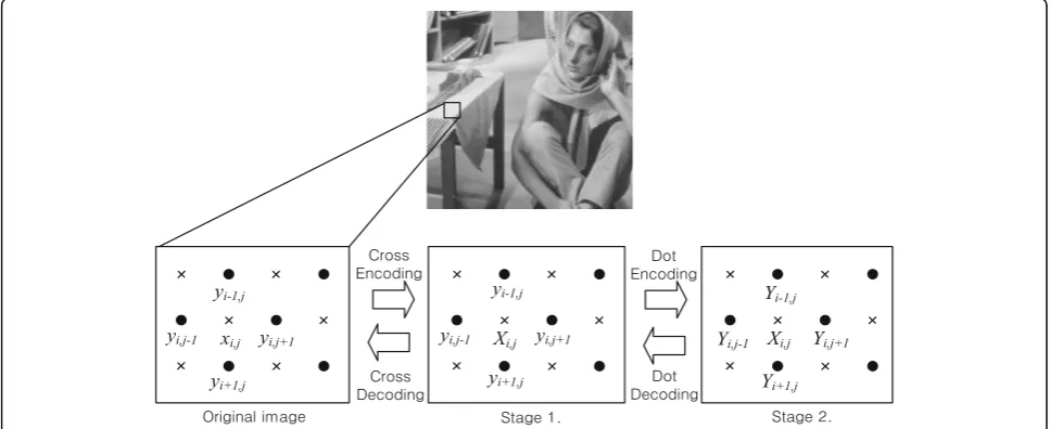
2.1 Two-stage embedding scheme using rhombus pattern Among fixed predictors, rhombus scheme has the best performance compared to other kinds of predictors such as GAP, MED, and CALIC [6]. In the rhombus pattern, two-stage embedding scheme was proposed by Sachnev et al. [8]. They divided an image into two kinds of non-overlapping sets of pixels with a rhombus pattern. In other words, it consists of two sets, so-called cross set and dot set as shown in Fig. 1. Their predicted value is obtained by the average value of four neighboring pixels around the target pixel. For example, a pixel which belongs to the cross set is predicted by the four closest pixels which belong to the dot set as shown in Fig. 1. Because of its effective grouping, it succeeds in
forming full context prediction and makes the out-standing improvement of the prediction accuracy over all other prediction methods which have support pixels including only the previous region of the target pixel. In other words, it is very difficult to design more advanced rhombus pattern predictor, despite the high-order modeling such as CALIC [7] and piecewise 2D auto-regression (P2AR) methods having many support pixels [6, 17, 18]. It turns out that accuracy of the predictor depends on not only the order but also the location of support pixels. Therefore, we adopt the rhombus pattern predictor and the two-stage embed-ding scheme in this paper.
2.2 Linear prediction
2.2.1 Least square approach
The coefficients for support pixels are computed adap-tively by the least square (LS) methods in linear predic-tion. It is one of the most advanced types of adaptive predictor, and it normally can provide better perform-ance than fixed predictors [6, 9]. The fixed predictor uses the fixed coefficients. However, adaptive predictor computes the coefficients dynamically according to the context.
In this paper, we use x(n) to denote a current target pixel, where n is the spatial coordinate in an image. Suppose that an image is scanned in a raster-scanning order, and x(n) is predicted by its causal neighboring pixels. According to the N-th order Markovian property, the predicted value is computed byNneighboring pixels as follows:
xpð Þ ¼n XN
k¼1
βð Þk x nð −kÞ; ð1Þ
whereβ(k) is a prediction coefficient for thek-th support pixel.
LS predictor works adaptively to the local features around the target pixel on a pixel-by-pixel basis [17]. In other words, the relations between each training set pixel and its support pixels are exploited usefully for predicting the relation between the target pixel and its support pixels as shown in Fig. 2.
The prediction coefficients are optimized locally inside each training set. A convenient choice of the training set is shown in Fig. 2 enclosed by blue lines, which contains
M= 2L(L+ 1) causal neighboring pixels. Let us denote the pixels in the training set by a M× 1 column vector as follows:
Y¼½y1ð Þn y2ð Þn ⋯ yMð ÞnT ð2Þ
Each pixel in the training set has the support pixels which consist of the N closest red-colored cross pixels as shown in Fig. 2. Then, the pixels in the training set and their support pixels would form anM×NmatrixX
as follows:
X¼
x1ðn−1Þ ⋯ x1ðn−NÞ
⋮ ⋯ ⋮
xMðn−1Þ ⋯ xMðn−NÞ 2
4
3
5 ð3Þ
where xj (n–k) is the k-th support pixel of training set pixel xj (n). The prediction coefficients are obtained through LS optimization inside the training set:
min kY−Xβk ð4Þ
It is a well-known fact that the P2AR optimization has a closed-form solution as follows:
β¼XTX−1XTY ð5Þ
where β= [β(1) β(2) ⋯ β(N)]T is the optimized predic-tion coefficients which have to be multiplied by the sup-port pixels. It provides an optimal prediction locally inside the training set.
2.2.2 Penalized regression using LASSO
Penalized regression methods aim at simultaneous vari-able selection in coefficient estimation. In practice, even if the sample size is small, a large number of support pixels are typically included to mitigate modeling biases. With such a large number of support pixels, there might exist multicollinearity problems among explanatory variablesX. Thus, selecting an appropriate size of the support pixels in a subset is desirable. Penalized regression can be an effective tool for such a selection.
Among methods that do both continuous shrinkage and variable selection, a promising technique called the LASSO was proposed by Tibshirani [24]. The LASSO is a penalized least squares procedure that minimizes the residual sum of squares (RSS) subject to the non-differentiable constraint expressed in terms of the L1 norm of the coefficients. That is, the LASSO estimator is given by
βL¼argminðY−XβÞ
0
Y−Xβ
ð Þ þ λXjp¼1βj ð6Þ
whereλ≥0 is a tuning parameter.
Regarding the choice of the best parameterλin Eq. (5), we utilize the Bayesian information criteria (BIC) intro-duced by Schwarz [25], through which we select a model that maximizes the posterior probability P[model| Y], where the model is subject to λ. Schwarz presents the approximation to the posterior probability for the iid (in-dependent and identically distributed) case:
BIC¼ −2⋅l ^β þ p⋅logð Þn; ð7Þ
where l β^ is the log-likelihood equation evaluated at the maximum likelihood estimate under the model of interest,pis the degree of freedom of our estimator, and nis the number of observations. It is interesting to note that the BIC adjusts the trade-off between the likelihood and the degree of sparseness so that the model maxi-mizes the posterior probability.
3 Proposed algorithm
Compared to existing reversible data hiding methods, the proposed method provides improved performance by using a more accurate predictor. The proposed idea is mainly based on two-stage embedding system of Sachnev et al.’s idea. We focus on improving prediction accuracy by:
Applying least square predictor which is able to obtain adaptive weigh for each support pixel. Applying LASSO penalized regression to least
square predictor on purpose of selecting the number and location of support pixels adaptively.
combined with the LS-based adaptive predictor [17] in the proposed method. Thus, support pixels of the pro-posed method consist of surrounding pixels aroundy(n) as shown in Fig. 3. A shape of a training set is shown in Fig. 4 in gray color.
Due to the property of two-stage embedding scheme [8], there are some pixels which should be excluded from the training set. Suppose that we embed a bit in dot set first. In Fig. 4, (in case of N =9), basically all pixels of the cross set in the past of target pixel can be
included in the training set and all pixels in the dot set such as E1,E2,E3,E4,E5, and E6 should be excluded from the training set because those pixels break reversibility. In other words, those pixels use at least one support pixel which is located in or behind target pixel.
Table 1The sample of prediction coefficients for support pixels Indexi x(n−i) βi
LS-based LASSO
0 N/A −26.393 −13.395
1 124 −0.022 0
2 84 0.337 0.228
3 123 0.499 0.458
4 77 0.417 0.374
5 95 0.459 0.434
6 141 −0.449 −0.312
7 98 0.073 0
8 146 −0.215 −0.084
9 113 0.168 0.021
10 46 −0.230 −0.086
11 84 −0.053 −0.069
12 59 0.154 0.094
13 73 −0.042 0
14 101 0.153 0.072
Fig. 5An example of a target pixel (in thered box) and its support pixels (N= 14)
Suppose that we have M training set pixels excluding the above improper pixels according to the sizeT. Each pixel has N support pixels. Then, it forms an M × N
matrix X as shown in Eq. (3). However, the proposed method applies one more idea to use more proper sup-port pixels for the purpose of improving the accuracy of the LS-based predictor.
3.2 Applying penalized regression via LASSO
LS-based prediction method, an adaptive predictor, can be improved by using penalized regression. In the proposed method, LASSO is utilized for penalized regression. LS predictor provides an adaptive coeffi-cient value, but penalized regression can make LS method be more adaptive. By the proposed method, we can penalize and remove some support pixels which are not influential to the target pixel. In other words, we can estimate the location of the most
critically influential support pixels as well as their prediction coefficients.
The following example explains how the proposed method achieves better performance. For example, in Fig. 5, when the target pixel valuey(n) is 83, its support pixel values arex(n−1) = 124,,x(n−2) = 84,∙andx(n−14) = 101 (see Fig. 3). Prediction coefficients are obtained from the LS-based approach and LASSO penalization. After the LASSO penalization, prediction coefficients for the blue colored pixels such asx(n-1),x(n-7), andx(n-13) become zero as shown in Table 1, which means that the number of the support pixels for the target pixel is reduced as shown in Fig. 6. The left-hand side and the right-hand side show the support pixels before and after the LASSO penalization, respectively. By removing the uncorrelated support pixels, prediction error gets smaller.
Table 1 shows that the coefficients of 124, 98, and 73 are smaller than others in magnitude. Thus,
Fig. 7Encoder and decoder of the proposed method
LASSO assigns 0 values to them and remove those pixels from the support pixels.
The LS-based approach calculates the predicted value xp as 74, and the LASSO penalization
calcu-lates it as 81 according to Eq. (1). LASSO estimates the target pixel more exactly because its given value is 83.
3.3 Encoder and decoder
This section describes the main step of the encoding and decoding processes. The proposed idea is explained more explicitly step by step with the description of the full process.
3.3.1 Encoder
Original image is divided into the cross set and the dot set for two-stage embedding as shown in Fig. 7. Embed-ding procedure starts at the cross set, and pixels are processed in raster-scanning order starting from the upper left corner. The cross set embedding procedure is as follows:
1. Compute local variance value for all pixels. Find the threshold value of the local variance values which is able to meet the embedding capacity.
2. Determine which pixels have smaller value of local variance comparing with the threshold value of local
Table 2Comparison in terms of average PSNR(dB) for low embedding capacities(lower than 0.5 bpp)
Image Sachnev et al. Lee et al. Dragoi and Coltuc Proposed
Sailboat 42.06 43.59 43.32 44.10
Barbara 45.32 46.75 46.19 47.01
Baboon 37.60 38.48 38.32 38.69
Boat 42.45 43.92 44.28 44.64
Pepper 42.09 44.19 44.30 44.40
Lena 46.96 46.94 47.32 47.33
Goldhill 44.26 44.06 44.76 44.76
Couple 44.34 44.55 45.02 44.84
House 50.21 50.44 49.67 50.69
Airplane 50.80 49.91 49.89 50.78
Elanie 40.75 42.76 42.35 42.95
Cameraman 55.11 54.55 55.24 54.60
Pirate 39.57 39.77 41.38 39.94
Tiffany 47.80 48.30 47.84 48.33
Average 44.95 45.59 45.71 45.93
Average gain 0.982 0.344 0.226 —
Table 3Comparison in terms of average PSNR(dB) for high embedding capacities(higher than 0.5 bpp)
Image Sachnev et al. Lee et al. Dragoi and Coltuc Proposed
Sailboat 33.83 34.38 34.72 35.13
Barbara 34.64 38.56 37.87 39.14
Baboon 28.38 29.71 29.17 29.92
Boat 34.46 36.37 36.23 36.92
Pepper 34.17 36.56 35.69 36.88
Lena 39.32 39.60 39.69 40.02
Goldhill 36.16 36.21 36.57 36.73
Couple 36.08 36.82 37.08 37.04
House 39.15 40.27 40.53 40.57
Airplane 42.25 42.18 42.17 42.41
Elanie 32.26 34.72 34.10 35.02
Cameraman 48.29 49.03 48.98 49.37
Pirate 32.47 33.02 33.47 33.20
Tiffany 38.58 40.42 39.42 40.45
Average 36.43 37.70 37.55 38.06
Average gain 1.625 0.354 0.508 —
variance. Only these pixels are available for embedding.
3. Computexp(n) using only a rhombus predictor [8] for the border pixels since training is not possible along the border. Computexp(n) using the proposed
algorithm for other pixels.
(a) Decide the training set with sizeLcentered on y(n) as shown in Fig.4.
(b)CreateXandYfrom the pixel values of the training set.
(c)Run LASSO estimator and obtain prediction coefficientβfor each support pixel.
(d)Computexp(n) using Eq. (1).
4. Compute the prediction error such as e(n) = x (n)−xp(n).
5. Embed a bit into the prediction error value using the prediction error expansion and histogram shift method.
6. Overflow and underflow problem has to be considered by using the location map bits such as Sachnev et al.’s method [8].
7. The pixels of the cross set are modified by
embedding associated bits as shown above. The dot
set embedding procedure starts with the same process. Obviously, training set includes the modified pixels of the cross set.
3.3.2 Decoder
Watermarked image is divided into the cross set and the dot set. Decoding procedure proceeds in the inverse order of the embedding procedure. In other words, dot set decoding proceeds first and cross set second.
The dot set decoding procedure is as follows. Ob-viously cross set and dot set are all modified by embedding.
1. Obtain the threshold value of the local variance, embedding capacity, and so on, from the side information.
2. Determine which pixels have smaller value of the local variance than the threshold value. Those pixels have the embedded bits.
3. In case of those pixels, computexp(n) using a
rhombus predictor [8] for the border pixels. Compute xp(n) using the proposed algorithm for other pixels.
4. Compute the modified prediction error such as e(n) =x(n)−xp(n).
5. Extract a bit out of the modified prediction error value using the prediction error expansion and histogram shift method. Original value of the target pixel is recovered.
6. Overflow and underflow problem has to be considered by using the location map bits such as Sachnev et al.’s method [8].
4 Experimental results
We implemented the reversible data hiding algorithms of Dragoi and Dinu [9], Sachnev et al. [8], Lee at el. [20], and the proposed method using MATLAB. We tested above four algorithms implemented on well-known 512 × 512 sized 8-bit grayscale images such as those shown in Fig. 8; Sailboat, Barbara, Baboon, Boat,
Pepper,Lena,Goldhill,Couple, andHouse. In addition,
Airplane, Elanie, Cameraman, Pirate, and Tiffany are also utilized for further experiments in Tables 2 and 3.
We embed the watermark message and side informa-tion as binary data in the images as a payload.
4.1 Effect of training set size,L
The effect of the training set sizeLfor the ttLASSO pre-diction vs. PSNR performance is analyzed. In the case of
Baboon¸ L=17 produces the best result as shown in Fig. 9. Without zooming, the PSNR results are almost close to each other, while significant gap exists in the zoomed result. The average PSNR difference between
L=17 and L=13 is 0.038 dB, and the average difference between 17 and 9 is 0.257 dB.
In all above test images, the value 13 or 17 is a proper compromise as the training set size for the best results. It means that LASSO-based LS method needs to have enough training set size to obtain the best effect.
4.2 Effect of the number of support pixel,N
The effect of the number of support pixel, N is quite significant. The greater number of support pixel, the better result in LASSO-based LS method. In the case of Barbara, PSNR result according to N is shown in Fig. 10. The average PSNR difference between N= 26 and N= 6 is 0.565 dB, and the average difference
between 26 and 14 is 0.199 dB. In all above test images,N= 26 has the best PSNR result. It means that LASSO-based LS method needs to have enough support pixels to obtain the best effect.
4.3 Comparison with other state-of-the-art schemes Let us compare the performance of the proposed scheme with other state-of-the-art schemes such as two-stage embedding scheme of [8] and other kinds of LS approaches of [9] and [20]. In the proposed method, following features are exploited:
1. LS predictor via LASSO with well-compromised size ofLandN
2. Two-stage embedding scheme with histogram shifting method [8]
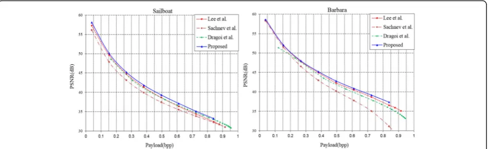
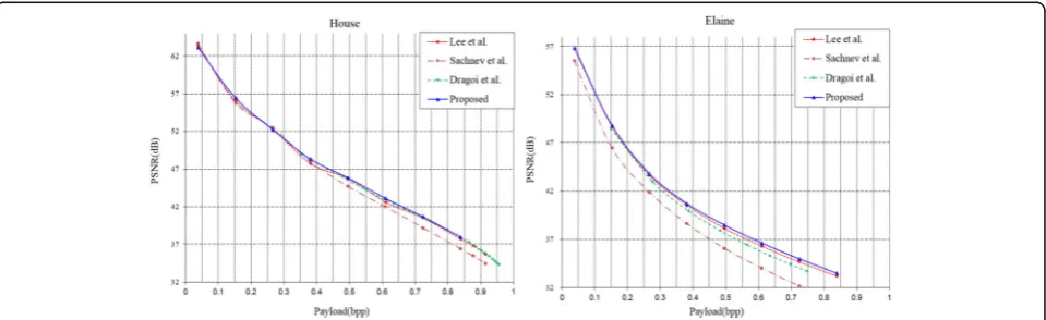
The comparison results with other schemes are shown in Figs. 11, 12, 13, and 14. It is manifested that the pro-posed method outperforms Sachnev et al.’s method [8]. In addition, the proposed method produces slightly
higher PSNR value than other least square methods [9, 20] only except a few cases of capacities on two of the test images such as Lena and Pepper. However, in terms of average gain in PSNR, the proposed method outper-forms the others on all test images of Fig. 8 with 1.82 dB over [8], 0.59 dB over [9], and 0.38 dB over [20].
To further verify the superiority of the proposed method, experimental results for high and low embedding capacities are listed in Tables 2 and 3. The average PSNR for low embedding capacities are computed by using 40,000, 70,000, 100,000, and 130,000 bits which are lower than 0.5 bpp in Table 2. On all test images of Table 2, the proposed method outperforms the others with an average gain in PSNR of 0.982 dB over [8], 0.344 dB over [20], and 0.226 dB over [9].
The average PSNR for high embedding capacities are computed by using 160,000, 190,000, and 220,000 bits which are higher than 0.5 bpp in Table 3. The result of high embedding capacities makes the superiority of the proposed method clearer. The proposed method out-performs the others with an average gain in PSNR of
1.625 dB over [8], 0.354 dB over [20], and 0.508 dB over [9].
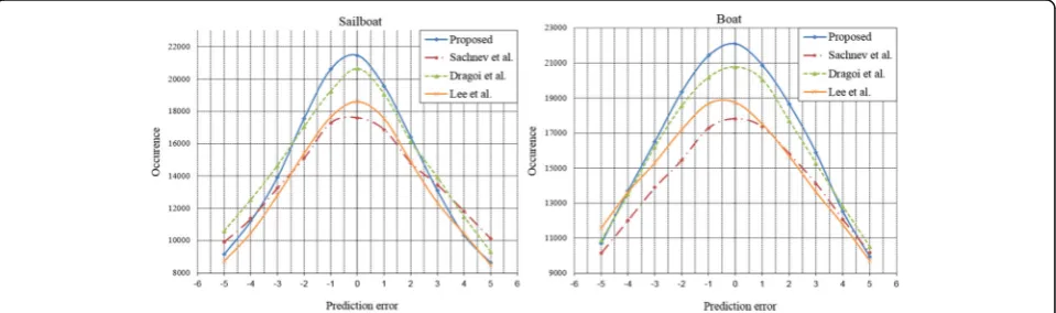
In addition, Figs. 15 and 16 confirms that the predictor in the proposed method has higher accuracy than those of Dragoi and Dinu’s method and Lee et al.’s method be-cause the proposed method results in higher occurrence of small prediction error values compared to others. The reasons why the proposed method outperforms other methods are summarized as follows.
First, the proposed method improves the state-of-the-art LS predictors [9] [20] via LASSO optimization. Dra-goi and Dinu’s method [9] and Lee et al.’s method [20] utilize the LS predictor using the different shape of training set and support pixels. However, the proposed method applies LASSO optimization to improve the pre-vious LS predictors. In most cases of images, the num-ber of support pixel, N =26 is selected for the best prediction performance in the proposed method while
N =4 [9] and N= 6 [20] are used in other LS predictor. In the proposed method, LASSO optimization selects the optimized support pixels to use and remove others. In other words, the proposed method is able to utilize
more proper support pixels out of many candidate sup-port pixels to increase accuracy of the LS computation.
5 Conclusions
In this paper, we proposed an enhanced predictor by using LASSO approach over normal LS predictor with rhombus-shaped two-stage embedding scheme. It en-ables finding out the shape of region around the target pixel and the proper weight coefficients. In other words, in the proposed method, it is possible to find reasonable number and location of the support pixels due to apply-ing LASSO into the LS approach. That is why a set of pixels located in highly variative region of image is pre-dicted more effectively by the proposed scheme rather than other LS predictors. Due to this property, the number of high prediction errors decreases. Thus, the proposed method has a tendency that significant im-provement happens in high embedding capacity, espe-cially in highly variative images. Experimental results demonstrate that the proposed method has better results than other state-of-the-art methods.
The authors declare that they have no competing interests.
About the authors Hee Joon Hwang
He received a B.S. degree in Electric and Electronic Engineering department in 2008 and a M.S. degree in Graduate School of Information Management and Security from Korea University, Seoul, Korea, in 2010. He joined at Graduate School of Information Security, Korea University, Seoul, Korea, in 2010, where he is currently pursuing Ph.D. His research interests include multimedia security, reversible and robust watermarking, and steganography. SungHwan Kim
He received a B.S. degree in Education department in 2007 and a M.S. degree in Statistics from Korea University, Seoul, Korea, in 2010. He received Ph. D. Biostatistics from University of Pittsburgh, Pittsburgh, in 2015. His research interests include methodological development for statistical machine learning methods, image processing, and optimization. Hyoung Joong Kim
He is currently with the Graduate School of Information Security, Korea University, Korea. He received his B.S., M.S., and Ph.D. from Seoul National University, Korea, in 1978, 1986, and 1989, respectively. He was a professor at Kangwon National University, Korea, from 1989 to 2006. He was a visiting scholar at University of Southern California, Los Angeles, USA, from 1992 to 1993. His research interests include data hiding such as reversible watermarking and steganography.
Author details
1
Graduate School of Information Security, Korea University, Seoul, South Korea.2Department of Statistics, Korea University, Seoul, South Korea.
Received: 1 June 2016 Accepted: 10 November 2016
References
1. J Tian, Reversible data embedding using a difference expansion. IEEE Trans. Circuits Syst. Video Technol.13(8), 890–896 (2003)
2. AM Alattar, Reversible watermark using difference expansion of triplets, in Proc. IEEE Int. Conf. Image Process. IEEE International Conference on Image Processing, Catalonia, Spain, 2003, vol. 1, pp. 501–504
3. AM Alattar, Reversible watermark using the difference expansion of a generalized integer transform. IEEE Trans. Image Process.13, 1147–1156 (2004) 4. DM Thodi, JJ Rodriguez, Expansion embedding techniques for reversible
watermarking. IEEE Trans. Image Process16(3), 721–730 (2007) 5. MJ Weinberger, G Seroussi, G Sapiro, The LOCO-I lossless image
compression algorithm:principles and standardization into JPEG-LS. IEEE Trans. Image Process.9(8), 1309–1324 (2000)
6. M Chen, Z Chen, X Zeng, Z Xiong, Model order selection in reversible image watermarking. IEEE J. Sel. Top. Signal Process.4(3), 592–604 (2010) 7. X Wu, N Memon, Context-based, adaptive, lossless image coding. IEEE Trans.
Commun.45(4), 437–444 (1997)
8. V Sachnev, HJ Kim, J Nam, S Suresh, YQ Shi, Reversible watermarking algorithm using sorting and prediction. IEEE Trans. Circuits Syst. Video Technol.19(7), 989–999 (2009)
9. IC Dragoi, D Coltuc, Local-prediction-based difference expansion reversible watermarking. IEEE Trans. Image Process.23(4), 1779–1790 (2014) 10. HJ Hwang, HJ Kim, V Sachnev, SH Joo, Reversible watermarking method
using optimal histogram pair shifting based on prediction and sorting. KSII, Trans. Internet Inform. Syst.4(4), 655–670 (2010)
11. SU Kang, HJ Hwang, HJ Kim, Reversible watermark using an accurate predictor and sorter based on payload balancing. ETRI J.34(3), 410–420 (2012)
optimization with edge-look-ahead. IEEE Trans. Circuits Syst.52(11), 751–755 (2005)
18. X Wu, G Zhai, X Yang, W Zhang, Adaptive sequential prediction of multidimensional signals with applications to lossless image coding. IEEE Trans. Image Process.20(1), 36–42 (2011)
19. J. Wen, L. Jinli, and W. Yi Adaptive reversible data hiding through autoregression, In Proceedings of 2012 IEEE International Conference on Information Science and Technology, ICIST. 2012. pp.831-838. 20. BY Lee, HJ Hwang, HJ Kim, Reversible data hiding using piecewise
autoregresive predictor based on two-stage embedding. J. Elect. Eng. Tech.
11(4), 974–986 (2016)
21. X Li, MT Orchard, Edge-directed prediction for lossless compression of natural images. IEEE Trans. Image Process.10(6), 813–817 (2001)
22. Z Ni, Y-Q Shi, N Ansari, W Su, Reversible data hiding. IEEE Trans, Circuits Syst.
16(3), 354–365 (2006)
23. Y-Q Shi, X Li, X Zhang, H-T Wu, B Ma, Reversible data hiding: advances in the past two decades. IEEE Access4, 3210–3237 (2016)
24. R Tibshirani, Regression shrinkage and selection via the lasso. J. Royal Stat. Soc., Series B58(1), 267–288 (1996)
25. G Schwarz, Estimating the dimension of a model. Ann Stat6(2), 461–464 (1978)
Submit your manuscript to a
journal and benefi t from:
7Convenient online submission
7Rigorous peer review
7Immediate publication on acceptance
7Open access: articles freely available online
7High visibility within the fi eld
7Retaining the copyright to your article