PERTURBATION ANALYSIS OF ”
k
−
ω” AND ”
k
−
”
TURBULENT MODELS.
WALL FUNCTIONS
Karel Vostruha1,aand Jaroslav Pelant1,b
1V´yzkumn´y a Zkuˇsebn´ı Leteck´y ´Ustav, VZL ´U,
Beranov´ych 130, 199 05 Praha - Letˇnany, Czech Republic
Abstract. Presented article shows rigorous method how derive non-stationary turbulent boundary layer equa-tions by perturbation analysis. The same method is used for analysing behaviour of ”k-omega” and ”k-epsilon” turbulent models. The analysis is divided into two parts: near wall behaviour - boundary conditions, and behaviour in ”log-layer” - wall functions. Both parts have important place in CFD. Boundary conditions are important part of CFD. ”k-omega” and ”k-epsilon” are related by one simple formula, but they yield to different solutions. Exact values for k, omega and epsilon on a wall are evaluated and all theoretical results are compared with numerical solutions. Special treatment is dedicated to ”k-epsilon” model and Dirichlet boundary condition for ”epsilon, instead of standard Neumann boundary condition. ”Log-Layer” is well known from experiments and it is used for setting constants in turbulent models. Standard equations are derived by perturbation analysis. In presented article are these equations derived with 3 more terms, than in standard case. This yields to sharper approxima-tion. These new equations are solved and solution is a bit different, than in standard case. Due to 3 extra terms is possible to get better approximation forkand new view into problematic..
1 Introduction
Two equations turbulent models are widely used in CFD - they give ”good” results in ”good” time. The most com-mon are ”k−ω” and ”k−ε”. This article is about turbulent boundary layer equations and perturbation analysis of tur-bulent models - on a wall and in ”log-layer”. Main goal is deriving Mathematical formulas for ”k”, ”ω” and ”ε”. on a wall - boundary conditions, and in “log-layer” - wall functions.
System of the Navier-Stokes equations in 2D with turbu-lent models
∂% ∂t +
∂(%u)
∂x + ∂(%v)
∂y =0 ∂u
∂t +
∂(%u2+p)
∂x +
∂(%uv)
∂y =
∂τxx
∂x + ∂τxy
∂y −
2 3
∂(%k)
∂x ∂v
∂t + ∂(uv)
∂x +
∂(%v2+p)
∂y =
∂τyx
∂x + ∂τyy
∂y −
2 3
∂(%k)
∂y ∂e
∂t +
∂(e+p)u
∂x +
∂(e+p)v
∂y =
∂
∂x(uτxx+vτxy)
+ ∂y∂(uτyx+vτyy)+
∂ ∂x
µ
Pr+ µT PrT
!∂ T ∂x !
+ ∂y∂ µ
Pr+ µT PrT
!∂ T ∂y !
Where
a e-mail:[email protected] b e-mail:[email protected]
τxx=(µ+µT) 4 3
∂u ∂x−
2 3
∂v ∂y !
τyy=(µ+µT) − 2 3
∂u ∂x+
4 3
∂v ∂y !
τxy=τyx=(µ+µT)
∂u ∂y+
∂v ∂x !
e=%ε+% 2(u
2+v2) ε= p
(κ−1)%
We need to close the Navier-Stokes equations by a turbu-lent model.
”k−ω” turbulent model:
∂(%k)
∂t + ∂(%ku)
∂x + ∂(%kv)
∂y =Pk+
∂
∂x (µ+σ ∗µ
T)
∂k ∂x !
+∂y∂ (µ+σ∗µT)
∂k ∂y !
−β∗%kω
∂(%ω)
∂t + ∂(%ωu)
∂x +
∂(%ωv)
∂y =α
ω kPk
+∂∂
x (µ+σµT) ∂ω
∂x !
+∂y∂ (µ+σµT)
∂ω ∂y !
−β%ω2
µT =
%k ω
”k−” turbulent model:
DOI: 10.1051/
C
Owned by the authors, published by EDP Sciences, 2013
epjconf 201/ 34501097
∂(%k)
∂t + ∂(%ku)
∂x +
∂(%kv)
∂y =Pk+
∂
∂x (µ+σ ∗µ
T)
∂k ∂x !
+ ∂y∂ (µ+σ∗µT)
∂k ∂y !
−β∗%
∂(%)
∂t + ∂(%u)
∂x +
∂(%v)
∂y =C1
kPk
+ ∂∂
x (µ+σµT) ∂ ∂x !
+∂y∂ (µ+σµT)
∂ ∂y !
−C2%
2
k
µT =Cν
%k2
Where
Pk=τxx
∂u ∂x+τxy
∂u ∂y+τyx
∂v ∂x+τyy
∂v ∂y
Model parametersα.β, β∗, σ, σ∗.C1.C2 are constants. kis
called kinetic turbulent energy, is called dissipation of turbulent energy.ωis called specific dissipation and it was introduced by Wilcox. Relation betweenandωis:ω= k.
Frequently used term is friction velocity defined asuτ = r
ν
∂u ∂y w.
2 Turbulent boundary layer
equations
We assume a smooth flat plate and a vicious, incompress-ible turbulent flow. We use neglecting method which is based on magnitudes of Reynolds number and distance from the wall.
Re= LV
ν ReT =
µT
µ
ReTis function of coordinates, but we assume for purposes of neglecting method, thatReT = √CRe. This approximation fits only in some hight up to the wall. Our goal is study-ing near wall behaver and we will see, that value of the constantC isn’t significant. We define the neglecting pa-rameter:
ε2= 1
Re
We introduce new variables
ξ= x
L N=
y Lε t˜=t
L V
Asymptotic expansion of (u, v):
¯ u= u
V =U1+εU2+· · · ¯
v= v
V =εV1+ε
2V 2+· · ·
We put new variables and asymptotic expansions into in-compressible turbulent the Navier-Stokes equations in non-dimensional form. We neglect all elements containing ε, then we get turbulent boundary layer equations:
∂U1
∂ξ + ∂V1
∂N =0 ∂U1
∂t˜ +U1
∂U1
∂ξ +V1
∂U1
∂N =− 1
% ∂pw
∂ξ + ∂
∂N (1+C) ∂U1
∂N !
p=pw−2 3%k
We should easily return to dimensional equations:
∂u ∂x +
∂v
∂y =0 (1)
∂u ∂t +u
∂u ∂x+v
∂u ∂y =−
1
% ∂pw
∂x + ∂
∂y (ν+νT)
∂u ∂y !
(2)
p=pw−2
3%k (3)
Equations (1) - (3) were derived without respect to used turbulent model. We can use the same method to ”k−ω” and ”k−” turbulent models and get behaviour of these models in the turbulent boundary layer
∂k ∂t +u
∂k ∂x+v
∂k
∂y =(ν+νT)
∂u ∂y
!2
+ ∂y∂ (ν+σ∗νT)
∂k ∂y !
−β∗kω
∂ω ∂t +u
∂ω ∂x +v
∂ω ∂y =α
ω k(ν+νT)
∂u ∂y
!2
+ ∂y∂ (ν+σνT)
∂ω ∂y !
−βω2 (4)
∂ ∂t +u
∂ ∂x+v
∂ ∂y=C
k(ν+νT)
∂u ∂y
!2
+∂y∂ (ν+σ∗νT)
∂ ∂y !
−C2
2
k (5)
3 Behaviour on a wall and
boundary conditions
We assume in all cases a stationary, incompressible flow, ∂
∂x ∂
∂y,vu. andνT ν. These assumptions are cor-rect and we will see another reason to use these assump-tions later. We starts with equation for ”ω”.
Comparing with DNS tells, thatω=O(y−α), velocity pro-file on wall is linear:u(y) = yu2τ
0=ν∂
2ω
∂y −βω2
We use ansatzω=Cy−αand it yields to:
ω= βy6ν2 (6)
Formula (6) is used for evaluating values of ω until the third line of cells.
We know, that turbulent kinetic energy decrease to 0 on a wall. We use previous assumptions for deriving equation forkand ansatzk=Cyα:
0= u
4
τ
ν +ν ∂2k
∂y2 −β
∗kω
k=u
4
τ
ν2
1
6ββ∗−2y
2 (7)
Equation foris from formula=kω.
= ν 3u4τ (3β∗−β)
Suitable boundary conditions are:k =0 or ∂k
∂n =0. If we use=kω, we see=O(1) and there is only one suitable boundary condition ∂∂n =0. Any Dirichlet boundary con-dition is unsuitable due to friction velocity. We will have to know values of friction velocity during all times. In case of boundary conditions is ”k−ω” better then ”k−” model. We can see from approximations forkandω, thatνT=O(y4).
4 Wall functions
Wall functions are approximations ofk,ωorin so-called ”log - layer”. Velocity profile is described by ” the law of the wall”u(y)=uτκ(lny+C). Whereκis von Karmar con-stant and concon-stant C depends on roughness of the wall and friction velocity. In this layer 1 ReT. Then equations are:
∂u ∂x +
∂v
∂y=0 (8)
u∂u ∂x +v
∂u ∂y =−
1
% ∂pw
∂x + ∂ ∂y
k ω
∂u ∂y !
(9)
u∂k ∂x +v
∂k ∂y=
k ω
∂u ∂y
!2 +σ∗ ∂
∂y k ω
∂k ∂y !
−β∗kω (10)
u∂ω ∂x +v
∂ω ∂y =α
∂u ∂y
!2
+∂y∂ ωk∂ω∂y !
−βω2 (11)
We assume an infinite plate parallel to the flow : pw = const., ∂∂x ∂y∂, ”log-layer”: u = uτκ (lny+C), then the system of equations is over-setted. It means, that we have 4 equations and 3 unknown functions. We will see, the sys-tem has point solution only on one line.
Equations (8) - (10) under the assumed ”log-layer” approx-imation have solution:
u=uτ
κ (lny+C1) v=C2 (12)
k=uτ κ
C2
√
β∗ln(C3y) (13)
ω= uτ
κ√β∗y (14)
σ∗=1 (15)
Equation (11) yields to point solution on the critical line:
ln(C3ycrit)=1− 1
σ+ uτ
κσ
√
β∗ C2
β β∗ −α
!
(16)
kon the critical line is:
kcrit= 1− 1
σ !
uτC2
κ√β∗+ u2
τ
κ2σ
β β∗ −α
!
(17)
We use well known formula for turbulent viscosity in ”log-layer”
νT =uτκy
Then we can evaluate:
C2 =
uτκ ln(C3ycrit)
=uτκσσ
−1 1−
√
β∗
σκ2
β β∗−α
!!
ln(C3ycrit)=
σ−1
σ 1−
√
β∗
σκ2
β β∗−α
!!−1
In light of the last formulated formulas and formula forkcrit we get
kcrit= u2τ
√
β∗ .
The right one wall functions on the critical line (y=ycrit) are:
u=uτ
κ(lny+C1)
v=uτκσσ
−1 1−
√
β∗
σκ2
β β∗ −α
!!
k= u
2
τ
√
β∗
ω= uτ κ√β∗y
Important is, we don’t need to know value of constantC3
for prescribing boundary conditions on the critical line. Standard wall functions fork−ωmodel. See Wilcox
∂u ∂x +
∂v ∂y =0
u∂u ∂x +v
∂u ∂y =−
1
u∂k ∂x +v
∂k ∂y=
k ω
∂u ∂y
!2 +σ∗ ∂
∂y k ω
∂k ∂y !
−β∗kω
u∂ω ∂x +v
∂ω ∂y =α
∂u ∂y
!2
+∂y∂ ωk∂ω∂y !
−βω2
With the same ”log-layer” assumptions.Solution (standard wall functions):
u= uτ
κ (lny+C1) v=0
k= u
2
τ
κ2σ
β β∗ −α
!
ω= uτ κ√β∗y
If we use limC2→0+ on solutions (12) - (14) and concept
of critical line (16), we get ”standard wall functions”. But
ycrit→+∞The limiting process shows, that presented the-ory is more complex and explain why ”standard wall func-tions“ yields to poor results. Another shape of this theory is impossibility to find extension under the same set up.
We have to figure out by experiment value of constantC1,
we don’t need to know value of constantC3, but we
as-sume it’s dependence onuτ. Value ofycrithas to evaluated from empirical formula. Following chapter shows limits Of ”simple” methods in boundary layer theory.
5 Impossibility theorem
We saw in previous section approximation of vertical part of velocity by a constant. In this section we formulate and prove theorem, that we can’t use any method of self-similar solutions, which are well known from laminar boundary layer theory
Theorem 1 Self-similar solutions can occur only in lami-nar boundary layer.
Proof We create proof by contradiction. Let exist a self-similar solution of an incompressible turbulent boundary layer equations described by this system of equations with a turbulent model.
∂u ∂x +
∂v ∂y=0
u∂u ∂x +v
∂u ∂y =−
1
% ∂pw
∂x + ∂
∂y (ν+νT)
∂u ∂y !
(18)
With a turbulent model, we don’t need equations from the turbulent model. We have these boundary conditions:
y = 0 : u=v=0, νT =0 pw(x)= f(x) x = 0 : u=U(0, y), v=0 νT =νT(0, y)
y→ ∞: u=U(x), v=0, νT =νT(∞)
We assume a self-similar solution, we need to find proper boundary conditions.. We can find parts of velocity in this form:
u=U(x)f y l(x)
!
(19)
v=U(x)l0(x) y l(x)f
0− d
dx(U(x)l(x))f (20)
We put formulas (19) and (20) into the equation (18) and we seek for self-similar solutions. It yields to this condi-tion:
l(x)
ν+νT
∂(ν+νT)
∂y =C
Solution is:
ν+νT =νexp Cy l(x)
!
ConstantC≤0, or we get infinite viscosity. It yields to this system of inequalities:
0≤νT =ν(exp Cy l(x) !
−1)≤0
We get contradiction - νT = 0 everywhere in turbulent boundary layer. We can see sharp border between methods of laminar and turbulent boundary layer.
6 Comparison and figures
We compare theoretical results with numerical solutions of compressible flow in this section. Main goal is check out how incompressible flow is good approximation for com-pressible flow. Numerical solution was done with k−ω
model with these constants: α = 59,β = 403, β∗ = 1009 ,
σ=σ∗ = 1
2. Computation mesh: 245 x 64. Outer velocity
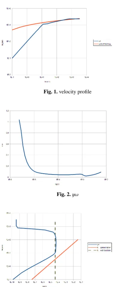
Fig. 1.velocity profile
Fig. 2.yω
Fig. 3.turbulent kinetic energy
We can see velocity profile ofu+ = u
uτ (blue curve) com-pared with ”log- profile” (red curve)in figure 1.κ =0.54, the value is much higher, than in literature.We can see one point intersection.
We can see evolution ofyω in figure 2. We can see con-stant part. We compared the value of concon-stant part with evaluated value forω:
ω− uτ
κ√β∗y
≈0.011
We can see evolution of the turbulent kinetic energy (blue curve) and comparison with standard wall function (bared line) forkin figure 3. The comparison is good due toκ = 0.54 - constant line. Wall behaviour (7) (orange curve) fails.
7 Conclusion
We saw in section 4 the most complex wall functions for k−ωmodel based on fully developed ”log-layer” and their link to ”standard wall functions”. These new wall functions explain problems in using standard ones and shows, that logarithmic approximation isn’t the best option fork−ω
model. Futher research will be focused on extending pre-sented theory on whole log-layer by using special pertur-bation functions. Setting boundary conditions on the criti-cal line is complicated for numericriti-cal solutions and prepar-ing commutation grids. The greatest disadvantage of all wall functions based on log- layer is strong assumption in stationary flow with fully developed log-layer. Near to point of separation or in non-stationary flows are standard boundary conditions better choice.
Compartment showed poor results and hightκ. We explain it as comparison of compressible and incompressible flow, not enough dense mesh,σ∗ = 0.5 insteadσ∗ =1 as was evaluated. More tests are required and work extension of new wall functions and change them by perturbation func-tions and constants into useful form in compressible flow. Then wall function become power tool in modelling of at-mosphere or other cases, where is problem to set boundary conditions on walls (surfaces)