Volume No.02, Issue No. 10, October 2014 ISSN (online): 2348 – 7550
AN ANALYTICAL STUDY OF LOSSY COMPRESSION
TECHINIQUES ON CONTINUOUS TONE
GRAPHICAL IMAGES
Dr.S.Narayanan
Computer Centre, Alagappa University, Karaikudi-South (India)
ABSTRACT
The programs using complex graphics consume prodigious amounts of disk storage. For example, the VGA
display is probably the current lowest common denominator for high-quality colour graphics. The VGA can
display 256 simultaneous colours selected from a palette of 262,144 colours. This lets the VGA display
continuous tone images, such as colour photographs, with a reasonable amount of fidelity. The problem with
using images of photographic quality is the amount of storage required to use them in a program. For example,
a 256-colour screen image has 200 rows of 320 pixels, each consuming a single byte of storage. This means
that a single screen image consumes a minimum of 64K. It isn’t hard to imagine applications that would
require literally hundreds of these images to be accessed. This paper discusses the use of some lossy image
compression techniques and also the analyzes the methods to achieve very high levels of data compression of
continuous tone graphical images such as digitized images of photographs. For this study, an image size of
64,000 Kbytes was taken as input image.
Keywords: Compression, DCT, Transform, Sub-Image
I. INTRODUCTION
Compression is the process of reducing the number of bits used to represent source image or the term data[1].
Compression also refers to the process of reducing the amount of data required to represent a given quality of
information. Data redundancy is a central issue in digital image compression. Based on the requirements, data
compression scheme can be divided into two broad classes. They are
1. Lossless Compression or Error Free Compression and
2. Lossy Compression or Error Compression.
1.1.1 Lossless Compression
This technique as the name implies involves no loss of data. That is these technique guaranteed to generate an
extract duplicate of input data stream after a compress/expanded cycle. This type of compression is used mostly
for data in database records, spreadsheets or word processing files.
1.1.2 Lossy Compression
This is the descriptive term for encoding and decoding process and procedures in which the output of decoding
procedure is not to be identical to the input. This technique involves some loss of information. Lossy
Volume No.02, Issue No. 10, October 2014 ISSN (online): 2348 – 7550
to facilitate compression. Lossy compression is generally done on analog data stored digitally, with the primaryapplications being graphics and sound files. In this paper, an experiment is presented to analyze and find out the
best technique for image compression among the available ones. This paper provides the substantial survey out
of all the image compression techniques. This approach will also provide the performance of every compression
techniques based on the various measurements. This paper is organized as follows : Section 1 gives the
introduction and illustrate the basic concept of Compression. Section 2 discusses about the transform coding
techniques. Next section (Section 3) illustrates the various existing compression standards. In Section 4 the
proposed experiment is explained. Section 5 discusses the result based on the performance of the compression
techniques on a given sample. Finally, the last section concludes.
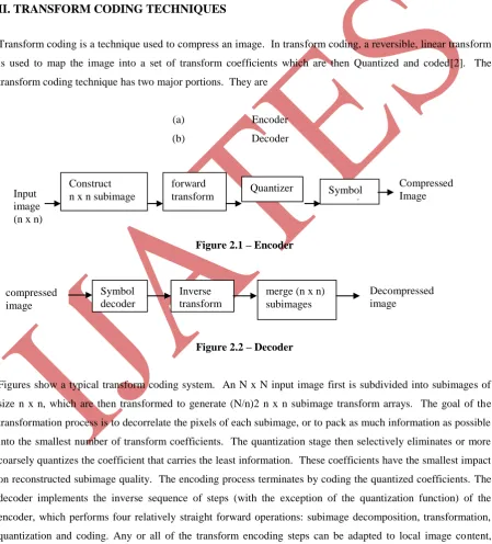
II. TRANSFORM CODING TECHNIQUES
Transform coding is a technique used to compress an image. In transform coding, a reversible, linear transform
is used to map the image into a set of transform coefficients which are then Quantized and coded[2]. The
transform coding technique has two major portions. They are
(a) Encoder
(b) Decoder
Figure 2.1 – Encoder
Figure 2.2 – Decoder
Figures show a typical transform coding system. An N x N input image first is subdivided into subimages of
size n x n, which are then transformed to generate (N/n)2 n x n subimage transform arrays. The goal of the
transformation process is to decorrelate the pixels of each subimage, or to pack as much information as possible
into the smallest number of transform coefficients. The quantization stage then selectively eliminates or more
coarsely quantizes the coefficient that carries the least information. These coefficients have the smallest impact
on reconstructed subimage quality. The encoding process terminates by coding the quantized coefficients. The
decoder implements the inverse sequence of steps (with the exception of the quantization function) of the
encoder, which performs four relatively straight forward operations: subimage decomposition, transformation,
quantization and coding. Any or all of the transform encoding steps can be adapted to local image content,
called adaptive transform coding, or fixed for all subimages called, non adaptive transform coding.
2.1 Various Types Of Transforms
Constructn x n subimage Input
image (n x n)
forward
transform Quantizer Symbol
encoder
Compressed Image
compressed image
Symbol decoder
Inverse transform
merge (n x n) subimages
Volume No.02, Issue No. 10, October 2014 ISSN (online): 2348 – 7550
1. Discrete Cosine Transform (DCT)2. Hadamard Transform
3. Walsh Transform
4. Haar Transform
5. Slant Transform
6. Orthogonal Polynomial Transform (OPT)
7. Fast Fourier Transform (FFT)
8. Karhunan – Loeve Transform (KL)
The major attribute in all of these image transforms is that the transform compacts the image energy to a few of
the transform domain samples.
III. COMPRESSION STANDARDS
3.1 JPEG Compression
The two standardization groups CCITT and the ISO, worked actively to get input from both industry and
academic groups concerned with image compression, and they seem to have avoided the potentially negative
consequences of their actions. The standard group created by these two organizations is the Joint Photographic
Experts Group (JPEG). It is the final stages of the standardization process. The JPEG specification consists of
several parts, including a specification for both lossless and lossy encoding[3]. The lossless coding uses the
predictive / adaptive model with Huffman code output stages, which produces a good compression of images
without the loss of any resolution.
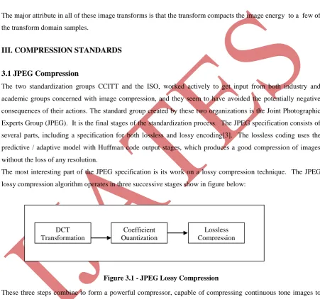
The most interesting part of the JPEG specification is its work on a lossy compression technique. The JPEG
lossy compression algorithm operates in three successive stages show in figure below:
Figure 3.1 - JPEG Lossy Compression
These three steps combine to form a powerful compressor, capable of compressing continuous tone images to
less than 10 of their original size, while losing little, if any, of their original fidelity.
3.2 Bi-Level (Binary) Image Compression Standards
The most widely used image compression standards are the CCITT group 3 and 4 standards for bi-level image
compression. Although they are currently utilized in a wide variety of computer applications, they were
originally designed as facsimile (FAX) coding methods for transmitting documents over telephone networks.
The group 3 standard applies a non adaptive, 1-D run-length coding technique where group 4 is a simplified
version of group 3 standard in which only D coding is allowed. Both standards uses the same non-adaptive
2-D coding approach.
3.3. Continuous Tone Image Compression Standards
DCTTransformation
DCT Transformation
DCT Transformation
Coefficient Quantization
Volume No.02, Issue No. 10, October 2014 ISSN (online): 2348 – 7550
The CCITT and ISO have defined several continuous tone image compression standards. These standardswhich are in various phases of the adoption process addresses both monochrome and colour image compressions
as well as still-frame and sequential frame applications. In contrast with the bi-level compression standards; all
continuous tone standards are based on the lossy transform coding techniques. To develop the standards,
CCITT and ISO committees solicited algorithm recommendations and the submitted standards represent the
state of art in continuous tone image compression. They deliver still-frame and sequential frame VHS –
compatible image quality with compression ratios of about 2:1 and 100:1 respectively.
IV. EXPERIMENT
In the N-by-N matrix, all the elements in row 0 have a frequency component of zero in one direction of the
signal. All the elements in column 0 have a frequency component of zero in the other direction. As the rows
and columns move away from origin, the coefficients in the transformed DCT matrix begin to represent higher
frequencies, with the highest frequencies found at position N-1 of the matrix. This is significant because most
graphical images on our computer screens are composed of low-frequency information. As it turns out, the
components found in row and column 0 (the DC components) carry more useful information about the image
than the higher-frequency components. As we move farther away from the DC components in the picture, we
find that the coefficients not only tend to have lower values, but they become far less important for describing
the picture. One of the first things that shown up when examining the DCT algorithm is that the calculation time
required for each element in the DCT is heavily dependent on the size of the matrix[4]. Since a doubly nested
loop is used, the number of calculations is O(N squared): as N goes up, the amount of time required to process
each element in the DCT output array will go up dramatically. One of the consequences of this is that it is
virtually impossible to perform a DCT on an entire image. The amount of calculation needed to perform a DCT
transformation on even a 256-by 256 grey-scale block is prohibitively large. To get around this, DCT
implementations typically break the image down into smaller, more manageable blocks. While increasing the
size of the DCT block would probably give better compression, it doesn’t take long to reach the point of
diminishing returns. Research shows that the connections between pixels even fifteen on twenty positions away
are of very little use as predictors. This means that a DCT block of 64-by-64 might not compress much better
than if we broke it down into four 16-by-16 blocks. And to make matters worse, the computation time would be
much longer. After applying DCT to the sub image we get the output matrix. The output matrix shows the
spectral compression characteristic the DCT is supposed to create. The “DC coefficient” is at position 0,0 in the
upper left hand corner of the matrix. This value represents an average of the overall magnitude of the input
matrix, since it represents the DC component in both the X and the Y axis. As the elements move farther and
farther from the DC coefficient, they tend to become lower and lower in magnitude. The next section discusses
how this can help to compress data.
4.1 Quantization
The “drastic” action used to reduce the number of bits required for storage of the DCT matrix is referred to as “Quantization”. Quantization is simply the process of reducing the number of bits needed to store an integer
value by reducing the precision of the integer. Once a DCT image has been compressed, we can generally
reduce the precision of the coefficients more and more as we move away from the DC coefficient at the origin.
Volume No.02, Issue No. 10, October 2014 ISSN (online): 2348 – 7550
Quantized value (i, j) =
)
,
(
)
,
(
j
i
Quantum
j
i
DCT
Rounded to nearest integer.
From the formula, it becomes clear that quantization values above twenty-five or perhaps fifty assure
that virtually all higher-frequency components will be rounded down to zero. Only if the high-frequency
coefficients get up to unusually large values will they be encoded as on-zero values.
During decoding, the dequantization formula operates in reverse
DCT(i,j) = Quantized Value (i,j) *Quantum (i, j)
4.2 Coding
The final step is coding the quantized images. The coding phase combines three different steps on the image.
The first changes the DC coefficient at 0,0 from an absolute value to a relative value. Since adjacent blocks in
an image exhibit a high degree of correlation, coding the DC element as the difference from the previous DC
element typically produces a very small number. Next, the coefficients of the image are arranged in the
“Zig-zag sequence”. Then they are enclosed using two different mechanisms. The first is run-length encoding of
zero values. The second is what JPEG calls “Entropy coding”. This involves sending out the coefficients codes,
using either Huffman coding or arithmetic coding depending on the choice of the implementer.
4.3 The Zig-Zag Sequence
One reason the JPEG algorithm compress so effectively is that a large number of coefficients in the DCT image
are truncated to zero values during the coefficient quantization stage[5]. So many values are set to zero that the
JPEG committee elected to handle zero values differently from other coefficient values. A simple code is
developed that gives a count of consecutive zero values in the image. Since over half of the coefficients are
quantized to zero in many images, this gives an opportunity for outstanding compression. One way to increase
the length of runs is to reorder the coefficients in the zig-zag sequence. Instead of compressing the coefficient
in row-major order, as a programmer would probably do, the JPEG algorithm moves through the block along
diagonal paths, selecting what should be the highest value elements first, and working its way toward the values
likely to be lowest. The diagonal sequences of quantization steps follow exactly the same lines, so the zig-zag
sequence should be optimal for our purposes.
4.4 Entropy Encoding
After converting the DC element to a difference from the last block, then reordering the DCT block in the
zig-zag sequence, the JPEG algorithm outputs the elements using an “entropy encoding” mechanism. The output
has RLE built into it as an integral part of the coding mechanism. Basically, the output of the entropy encoder
consists of a sequence of three tokens, repeated until the block is complete. The three tokens look like this:
Run Length : The number of consecutive zeros that preceded the current elements in the DCT output matrix.
Bit Count : The number of bits to follow in the amplitude number.
Volume No.02, Issue No. 10, October 2014 ISSN (online): 2348 – 7550
The coding sequence used here is a combination of Huffman coding and variable length integer coding. Therun-length and bit-count values are combined to form a Huffman code that is output. The bit count refers to the
number of bits used to encode the amplitude as a variable-length integer. The variable-length integer coding
scheme takes advantage of the fact that the DCT output should consist of mostly smaller numbers, which we
want to encode with smaller numbers of bits. The bit counts and the amplitudes which they encode follow.
Likewise, all the transforms are encoded and decoded in this way of sequence.
V. TABLES AND FIGURES
Table 1: Comparison of Compression Ratio and Output Bytes for the Various Transforms with Quality Factor 5 and Image Size 4
Transform Compression Ratio in
%
Output Bytes
DCT 63 24212
HAAR 68 22932
HADAMARD 12 56937
WALSH 62 24783
SLANT 49 33181
OPT 86 9713
Table 2: Comparison of Compression Ratio and Output Bytes for the Various Transforms with Quality Factor 15 and Image Size 4
Transform Compression Ratio in
%
Output Bytes
DCT 76 15717
HAAR 79 16170
HADAMARD 33 43432
WALSH 75 16629
SLANT 69 19876
OPT 90 6659
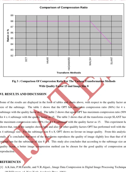
Table 3: Comparison of Compression Ratio and Output Bytes for the Various Transforms with Quality Factor 15 and Image Size 8
Transform Compression Ratio in
%
Output Bytes
DCT 88 8211
HAAR 88 9751
HADAMARD 88 8043
WALSH 88 8153
Volume No.02, Issue No. 10, October 2014 ISSN (online): 2348 – 7550
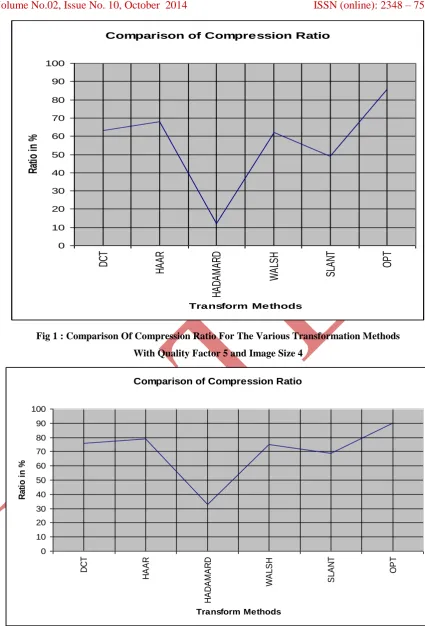
Comparison of Compression Ratio
0 10 20 30 40 50 60 70 80 90 100
DCT
H
A
A
R
H
A
D
A
M
A
R
D
W
A
LS
H
S
LA
N
T
O
P
T
Transform MethodsR
at
io
in
%
Fig 1 : Comparison Of Compression Ratio For The Various Transformation Methods With Quality Factor 5 and Image Size 4
Comparison of Compression Ratio
0 10 20 30 40 50 60 70 80 90 100 DCT H A A R H A D A M A R D W A L S H S L A N T O P T Transform Methods R a ti o in %
Volume No.02, Issue No. 10, October 2014 ISSN (online): 2348 – 7550
Comparison of Compression Ratio
82 83 84 85 86 87 88 89
DCT
H
A
A
R
H
A
D
A
M
A
R
D
W
A
L
S
H
S
L
A
N
T
Transform Methods
R
a
ti
on
i
n
%
Fig 3 : Comparison Of Compression Ratio For The Various Transformation Methods With Quality Factor 15 and Image Size 8
VI. RESULTS AND DISCUSSION
Some of the results are displayed in the form of tables and charts above, with respect to the quality factor and
size of the subimage. The table 1 shows that the OPT has maximum compression ratio (86%) for 4 x 4
subimage with the quality factor as 5. The table 2 shows that again OPT has maximum compression ratio (90%)
for 4 x 4 subimage with the quality factor as 15. The table 3 shows that all the transforms except SLANT have
the maximum compression ratio (88%) for 8 x 8 subimage with the quality factor as 15. This experiment has
shown that, out of the samples shown here and also for other qualifty factors OPT has performed well with the 4
x 4 subimage size. For the subimage size 8 x 8, OPT shows no favour on image quality. From this analytical
study, it is concluded that most of the transforms reproduces the quality of image slightly less than that of the
original one for the subimage of size 8 x 8. This study also concludes that according to the subimage size and
quality factor, a better image compression method can be chosen for the good quality of compression and
reproduction.
REFERENCES
[1] A.K.Jain, P.M.Farrelle, and V.R.Algazi., Image Data Compression in Digital Image Processing Techniques
(M.P.Ekstrom, ed. New York; Academic Press, 1984).
[2] Clark, R.J. , Transform Coding of Images (Academic Press, New York, 1985).
[3] Mark Nelson, Jean-Loup Gailly, The Data Compression Book (Second ed. Bpb publications, 1996).
[4] Ahmed, N., Natarajan, T., and Rao, K.R., Discrete Cosine Transforms, IEEE Trans. Comp. Vol. C-23,
1974, pp. 90-93.