From Weak to Strong Linear Programming Gaps for All Constraint Satisfaction Problems

www.theoryofcomputing.org

S

: CCC 2017

From Weak to Strong

Linear Programming Gaps for All

Constraint Satisfaction Problems

Mrinalkanti Ghosh

Madhur Tulsiani

Received July 30, 2017; Revised May 8, 2018; Published June 6, 2018

Abstract: We study the approximability of constraint satisfaction problems (CSPs) by linear programming (LP) relaxations. We show that for every CSP, the approximation obtained by a basic LP relaxation is at least as strong as the approximation obtained using relaxations given byc·logn/log lognlevels of the Sherali–Adams hierarchy (for some constantc>0) on instances of sizen.

It was proved by Chan et al. [FOCS 2013] (and recently strengthened by Kothari et al. [STOC 2017]) that for CSPs, any polynomial-size LP extended formulation is at most as strong as the relaxation obtained by a constant number of levels of the Sherali–Adams hierarchy (where the number of levels depend on the exponent of the polynomial in the size bound). Combining this with our result also implies that any polynomial-size LP extended formulation is at most as strong as thebasicLP, which can be thought of as the base level of A conference version of this paper appeared in the Proceedings of the 32nd Computational Complexity Conference (CCC’17) [14].

∗_{NSF award number CCF-1254044.}

†_{NSF award number CCF-1254044.}

ACM Classification:F.2.2, G.1.6 AMS Classification:68Q17, 90C05

the Sherali–Adams hierarchy. This essentially gives a dichotomy result for approximation of CSPs by polynomial-size LP extended formulations.

Using our techniques, we also simplify and strengthen the result by Khot et al. [STOC 2014] on (strong) approximation resistance for LPs. They provided a necessary and sufficient condition under which o(log logn)levels of the Sherali–Adams hierarchy cannot achieve an approximation better than a random assignment. We simplify their proof and strengthen the bound to o(logn/log logn)levels.

1

Introduction

Given a finite alphabet[q] ={0, . . . ,q−1}and a predicate f :[q]k→ {0,1}, an instance of the problem MAX k-CSP(f) consists ofmconstraints over a set ofnvariables,x1, . . . ,xn, taking values in the set

[q]. Each constraintCiis of the form f(xi1+bi1, . . . ,xik+bik)for somek-tuple(xi1, . . .xik)of variables,

and constantsbi1, . . . ,bik∈[q], where the addition is taken to be moduloq. We say that an assignment

σ to the variables satisfies the constraintCi ifCi(σ(xi1), . . . ,σ(xik)) =1. Given an instanceΦof the

problem, the goal is to find an assignmentσ to the variables satisfying as many constraints as possible.

The approximability of theMAX k-CSP(f)problem has been extensively studied for various predicates

f (see, e. g., [30] for a survey), and special cases include several interesting and natural problems such as MAX 3-SAT,MAX 3-XORandMAX-CUT.

A topic of much recent interest has been the efficacy of Linear Programming (LP) and Semidefinite Programming (SDP) relaxations. For a given instanceΦ ofMAX k-CSP(f), letOPT(Φ) denote the

fractionof constraints satisfied by an optimal assignment, and letFRAC(Φ) denote the value of the convex (LP/SDP) relaxation for the problem. Then, the performance guarantee of this algorithm is given by theintegrality gapwhich equals the supremum ofFRAC(Φ)/OPT(Φ), over all instancesΦ.

The study of unconditional lower bounds for general families of LP relaxations was initiated by Arora, Bollobás and Lovász [2] (see also [3]). They studied the Lovász-Schrijver [25] LP hierarchy and proved lower bounds on the integrality gap forMinimum Vertex Cover(their technique also yields similar bounds forMAX-CUT). De la Vega and Kenyon-Mathieu [12] and Charikar, Makarychev and Makarychev [9] proved a lower bound of 2−o(1)for the integrality gap of the LP relaxations for MAX-CUTgiven respectively by O(log logn)andnO(1)levels of the Sherali–Adams LP hierarchy [29]. Several follow-up papers have also shown lower bounds for various other special cases of theMAX k-CSPproblem, both for LP and SDP hierarchies [1,28,33,27,6,5,22].

An LP extended formulation of a polytopeP⊆_Rd_{is a linear program of the form} Ex+Fy = g and E0x+F0y ≤ g0,

wherex∈_Rd_,y∈

Rt, andx∈Pif and only if there existsysuch that(x,y)is a solution to the above LP. We take the size of an LP extended formulation to be the sum of the number of variables and the number of constraints (equalities plus inequalities). We refer the interested reader to a discussion in [13] for different (equivalent) notions of size.

gap, but for the entireapproximability curve. We say thatΦ is (c,s)-integrality gap instancefor a relaxation ofMAX k-CSP(f), if we have

FRAC(Φ) ≥ c and OPT(Φ) < s.

And we say that Φ is (c,s)-approximable by a relaxation of MAX k-CSP(f), if for instances with OPT(Φ)<s, we haveFRAC(Φ)≤c. They showed that for any fixedt∈_N, if there exist(c,s)-integrality gap instances of sizenfor the relaxation given bytlevels of the Sherali–Adams hierarchy, then for all

ε>0 and sufficiently largeN, there exists a(c−ε,s+ε)-integrality gap instance of size (number of

variables)N, for any linear extended formulation of size at mostNt/2. They also give a trade-off whentis a function ofn. This was recently improved by Kothari et al. [21] and we describe the improved trade-off later.

We strengthen the above results by showing that for allc,s∈[0,1],(c,s)-integrality gap instances for a “basic LP” can be used to construct(c−ε,s+ε)-integrality gap instances forΩε(logn/log logn)

levels of the Sherali–Adams hierarchy. The basic LP uses only a subset of the constraints in the relaxation given byklevels of the Sherali–Adams hierarchy forMAX k-CSP(f). In particular, this shows that a lower bound on the integrality gap for even the basic LP implies a similar lower bound on the integrality gap of any polynomial-size extended formulation. This can also be viewed as a dichotomy result showing that for any predicate f, eitherMAX k-CSP(f)is(c,s)-approximable by thebasic LP relaxation(where the number of LP variables and constraints are linear in the size of the instance) or for allε >0, a

(c−ε,s+ε)-approximation cannot be achieved byany polynomial-size LP extended formulation. We note that both the above results and our result apply to all f,qand allc,s∈[0,1].

1.1 Comparison with (implications of) Raghavendra’s UG-hardness result

A remarkable result by Raghavendra [26] shows that a(c,s)-integrality gap instance for a “basic SDP” relaxation ofMAX k-CSP(f) implies Unique-Games-hardness (UG-hardness) [16] of distinguishing instancesΦwithOPT(Φ)<sfrom instances withOPT(Φ)≥c. The basic SDP considered by Raghaven-dra involves moments for all pairs of variables and all subsets of variables included in a constraint. The basic LP we consider is weaker than this SDP and does not contain the positive semidefiniteness constraint.

Combining Raghavendra’s result with known constructions of integrality gaps for Unique Games by Raghavendra and Steurer [27], and by Khot and Saket [17], one can obtain a result qualitatively similar to ours, for the mixed hierarchy. In particular, a(c,s)-integrality gap for the basic SDP implies a (c−ε,s+ε)-integrality gap forΩ((log logn)1/4)levels of the mixed hierarchy.

Note however, that the above result is incomparable to our result, since it starts with stronger hypothesis (a basic SDP gap) and yields a gap for the mixed hierarchy as opposed to the Sherali–Adams hierarchy. While the above can also be used to derive lower bounds for linear extended formulations, one needs to start with an SDP gap instance to derive an LP lower bound. The basic SDP is known to be provably stronger than the basic LP for several problems including various 2-CSPs. Also, for the worst case f forq=2, the integrality gap of the basic SDP is O(2k_{/k)[10], while that of the basic LP is 2}k−1_.

The integrality gap for the basic LP is achieved by “all zero or all one” predicate.

implies UG-hardness of distinguishing instancesΦ withOPT(Φ)≥Ω c/(k3·logq)from instances withOPT(Φ)≤4s. Their result also shows that a(c,s)-integrality gap instance for the basic LP can be used to produce a Ω c/(k3·logq),4s-integrality gap instance for the basic SDP, and hence for Ω((log logn)1/4_{)levels of the mixed hierarchy.}

1.2 Other related work

The power of the basic LP for solving valued CSPsto optimalityhas been studied in several previous papers. These results concerns the problem of minimizing the penalty for unsatisfied constraints, where the penalties take values inQ∪ {∞}. Also, they study the problem not only in terms of single predicate f, but rather in terms of the constraint language generated by a given set of (valued) predicates.

It was shown by Thapper and Živný [31] that when the penalties are finite-valued, if the problem of finding the optimum solution cannot be solved by the basic LP, then it isNP-hard. Kolmogorov, Thapper and Živný [20] give a characterization of CSPs where the problem of minimizing the penalty for unsatisfied constraints can be solvedexactlyby the basic LP. Also, a recent result by Thapper and Živný [32] shows that the valued CSP problem for a constraint language can be solved to optimality by a bounded number of levels of the Sherali–Adams hierarchy if and only if it can be solved by a relaxation obtained by augmenting the basic LP with constraints implied by three levels of the Sherali–Adams hierarchy. However, the above papers only consider the case when the LP gives an exact solution, and do not focus on approximation.

The techniques from [9] used in our result, were also extended by Lee [24] to prove a hardness for the Graph Pricing problem. Kenkre et al. [15] also applied these to show the optimality of a simple LP-based algorithm for Digraph Ordering.

1.2.1 Our results

Our main result is the following theorem, which shows that for every CSP, for instances of sizen, the basic LP is at least as strong as any relaxation given by o(logn/log logn)levels of the Sherali–Adams hierarchy.

Theorem 1.1. Let f :[q]k_{→ {0,1}be any predicate. Let}

Φ0be a(c,s)-integrality gap instance for basic

LP relaxation ofMAX k-CSP(f). Then for everyε >0, there exists cε >0 such that for infinitely

manyN∈_N, there exist(c−ε,s+ε)-integrality gap instances of sizeNfor the LP relaxation given by

cε·logN/log logNlevels of the Sherali–Adams hierarchy.

Combining the above with the connection between Sherali–Adams gaps and extended formulations by [7, 21] also yields that the basic LP is at least as strong as any LP extended formulation of size

no(logn/log logn).

Corollary 1.2. Let f :[q]→ {0,1}be any predicate. LetΦ0be a(c,s)-integrality gap instance for basic LP relaxation ofMAX k-CSP( f ). Then for everyε>0, there exists c0_ε>0such that for infinitely many N∈N, there exist(c−ε,s+ε)-integrality gap instances of size N, for every linear extended formulation

As an application of our methods, we also simplify and strengthen the approximation resistance results for LPs proved by Khot et al. [19]. They studied predicates f :{0,1}k_{→ {0,1}and provided}

a necessary and sufficient condition for the predicate to bestrongly approximation resistantfor the Sherali–Adams LP hierarchy. One says a predicate is strongly approximation resistant if for allε>0, it

is hard to distinguish instancesΦfor which

OPT(Φ)− _E

x∈{0,1}k[f(x)]

≤ ε

from instances withOPT(Φ)≥1−ε. In the context of the Sherali–Adams hierarchy, they showed that

when this condition is satisfied, there exist instancesΦsatisfying

OPT(Φ)− _E

x∈{0,1}k[f(x)]

≤ ε and FRAC(Φ) ≥ 1−ε,

where FRAC(Φ) is the value of the relaxation given by Oε(log logn) levels of the Sherali–Adams

hierarchy. We strengthen their result (and provide a simpler proof) to prove the following.

Theorem 1.3. Let f :{0,1}k_{→ {0,1}be any predicate satisfying the condition for strong approximation} resistance for LPs, given by [19]. Then for everyε>0, there exists cε >0such that for infinitely many N∈_N, there exists an instanceΦofMAX k-CSP(f)of size N, satisfying

OPT(Φ)− _E

x∈{0,1}k[f(x)]

≤ ε and FRAC(Φ) ≥ 1−ε,

whereFRAC(Φ)is the value of the relaxation given by cε·logN/log logN levels of the Sherali–Adams hierarchy.

As before, the above theorem also yields a corollary for extended formulations.

1.2.2 Proof overview and techniques

The gap instance. The construction of our gap instances is inspired by the construction by Khot et al. [19]. They gave a generic construction to prove integrality gaps for any approximation resistant predicate (starting from certificates of hardness in form of certain “vanishing measures”), and we use similar ideas to give a construction which can start from a basic LP integrality gap instance as a certificate, to produce a gap instance for a large number of levels. This construction is discussed inSection 5.

Given an integrality gap instanceΦ0onn0variables, we treat this as a “template” (as in

Raghaven-dra [26]) and generate a random instance using this. Concretely, we generate a new instanceΦonn0sets

ofnvariables each. To generate a constraint, we sample a random constraintC0∈Φ0, and pick a variable

randomly from each of the sets corresponding to variables inC0. Thus, the instances generated are n₀-partite random hypergraphs, with each edge being generated according to a specified “type” (indices of sets to chose vertices from).

However, proving an LP/SDP lower bound using such instances implies a strong result: The predicate f is

uselessfor the corresponding relaxation, in the sense defined by [4] (replacing the “P6=NP” assumption by the assumption that UG does not belong toP). Uselessness only holds for a limited class of predicates

f (when f−1(1)supports a balanced pairwise independent distribution on[q]k) [4]. Thus, proving an SDP lower bound for predicates which are not expected to be useless requires a new construction of instances, which cannot be generated uniformly at random. Our construction provides such a generalization, and may be useful in proving new SDP lower bounds. The properties of randomGn,phypergraphs easily carry

over to our instances, and we collect these properties inSection 3.

The above construction ensures that if the instanceΦ0does not have an assignment satisfying more

than ansfraction of the constraints, thenOPT(Φ)≤s+ε with high probability. Also, it is well-known

that providing a good LP solution to the relaxation given bytlevels of the Sherali–Adams hierarchy is equivalent to providing distributionsDS on[q]S for all sets of variables S with|S| ≤t, such that

the distributions are consistent restricted to subsets, i. e., for allSwith|S| ≤tand all T ⊆S, we have

DS|T =DT. Thus, in our case, we need to produce such consistent local distributions such that the

expected probability that a random constraintC∈Φis satisfied by the local distribution on the set of variables involved inC(which we denote asSC) is at leastc−ε.

Local distributions from local structure. Most papers on integrality gaps for CSPs utilize the local structure of random hypergraphs to produce such distributions. Since the girth of a sparse random hypergraph isΩ(logn), any induced subgraph on o(logn)vertices is simply a forest. In case that the induced hypergraphGSon a setSis atree, there is an easy distribution to consider: simply choose an

arbitrary root and propagate down the tree by sampling each child conditioned on its parent. It is also easy to see that forT ⊆S, if the induced hypergraphGT is asubtreeofGS, then the distributionsDSand DT produced as above are consistent.

The extension of this idea to forests requires some care. One can consider extending the distribution to forests by propagating independently on each tree in the forest. However, if forT ⊆S GT is a forest

whileGSis a tree, then a pair of vertices disconnected inGT will have no correlation inDT but may

be correlated inDS. This was handled, for example, in [19] by adding noise to the propagation and

using a large ballB(S)aroundSto defineDS. Then, if two vertices ofT are disconnected inB(T)but

connected inB(S), then they must be at a large distance from each other. Thus, because of the noise, the correlation between them (which is zero inDT) will be very small in DS. However, correcting

approximate consistency to exact consistency incurs a cost which is exponential in the number of levels (i. e., the sizes of the sets), which is what limits the results in [19,12] to O(log logn)levels. This also makes the proof more involved since it requires a careful control of the errors in consistency.

Consistent partitioning schemes. We resolve the above consistency issue by first partitioning the given setSinto a set of clusters, each of which have diameter∆H=o(logn)in the underlying hypergraph H. Since each cluster has bounded diameter, it becomes a tree when we add all the missing paths between any two vertices in the cluster. We then propagate independently on each cluster (augmented with the missing paths). This preserves the correlation between any two vertices in the same cluster, even if the path between them was not originally present inGS.

restriction toT of partition obtained for the setS. In fact, we construct distributions over partitions

{PS}|S|≤t, which satisfy the consistency propertyPS|T =PT. These distributions over partitions, which

we callconsistent partitioning schemes, are constructed inSection 4.

In addition to being consistent, we require that the partitioning scheme cuts only a small number of edges in expectation, since these contribute to a loss in the LP objective. We remark that such low-diameter decompositions (known asseparatingandpaddeddecompositions) have been used extensively in the theory metric embeddings (see, e. g., [23] and the references therein). The only additional requirement in our application is consistency.

We obtain the decompositions by proving the (easy) hypergraph extensions the results of Charikar, Makarychev and Makarychev [11], who exhibit a metric which is similar to the shortest path metric on graphs at small distances, and has the property that its restriction to any subset of size at mostnε0 _(for

an appropriateε0<1) is`2embeddable. This is proved inSection 3. A variant of this metric was used

by Charikar, Makarychev and Makarychev [9] to prove lower bounds forMAX-CUT, fornε0 _{levels of}

the Sherali–Adams hierarchy. They used the embedding to construct a “local SDP solution” for anynε0

variables (with value 1−ε0) and produced the distributions required for Sherali–Adams by rounding the

SDP solutions (which gives value 1−O(√ε0)). However, rounding an SDP solution with a high value

does not always produce a good integral solution for other CSPs.

Instead, we use these metrics inSection 4to construct the consistent partitioning schemes as described above, by applying a result of Charikar et al. [8] giving separating decompositions for finite subsets of `2. We remark that it is the consistency requirement of the partitioning procedure that limits our results

to O(logn/log logn)levels. The separation probability in the decomposition procedure grows with the dimension of the`2embedding, while (to the best of our knowledge) dimension reduction procedures

seem to break consistency.

2

Preliminaries

We use[n]to denote the set{1, . . . ,n}. The only exception is[q], where we overload this notation to denote the set{0, . . . ,q−1}, which corresponds to the the alphabet for the Constraint Satisfaction Problem under consideration. We useDSandPSto denote probability distributions over assignments

to and partitions of a setS, respectively. ForT ⊆S, the notationDS|T is used to denote the restriction

(marginal) of the distributionDSto the setT (and similarly forPS|T).

2.1 Constraint Satisfaction Problems

Definition 2.1. Let[q]denote the set{0, . . . ,q−1}. For a predicate f :[q]k→ {0,1}, an instanceΦof MAX k-CSPq(f)consists of a set{x1, . . . ,xn}of variables and a set{C1, . . . ,Cm}of constraints. Each

constraintCiis over ak-tuple(xi1, . . . ,xik)of variables, and the constraint is of the form

Ci ≡ f(xi1+bi1, . . . ,xik+bik)

for somebi1, . . . ,bik∈[q], where the addition is moduloq. For an assignmentσ:[n]7→[q], letsat(σ)

maximize E C∈Φ





∑

α∈[q]k

f(α+bC)·x(SC,α)





∑

α∈[q]S

α|T=β

x_(S,α) = x_(T,β) ∀T⊆S⊆[n],|S| ≤t,∀β∈[q]T

x(S,α) ≥ 0 ∀S⊆[n],|S| ≤t,∀α∈[q]S

x_(/0,/0) = 1

Figure 1: Level-tSherali–Adams LP forMAX k-CSPq(f).

of constraints that can be simultaneously satisfied is denoted byOPT(Φ), i. e.,

OPT(Φ) = max

σ:[n]7→[q]sat(σ).

For a constraintCof the above form, we usexCto denote the tuple(xi1, . . . ,xik)of variables, andbC

to denote the tuple(bi1, . . . ,bik). We then write the constraint as f(xC+bC). We also denote bySCthe set

of indices,{i1, . . . ,ik}, of the variables participating in the constraintC.

2.2 The LP relaxations for Constraint Satisfaction Problems

Below we present various LP relaxations for theMAX k-CSPq(f)problem that are relevant in this paper.

We start with the level-tSherali–Adams relaxation. The intuition behind it is the following. Note that an integer solution to the problem can be given by an assignmentσ:[n]→[q]. Using this, we can

define{0,1}-valued variablesx₍S,α)for eachS⊆[n],1≤ |S| ≤tandα∈[q]S, with the intended solution

x₍S,α)=1 ifσ(S) =α and 0 otherwise. We also introduce a variablex(/0,/0), which equals to 1. We relax the integer program and allow variables to take real values in[0,1]. Now the variables{x_(S,α)}_α∈[q]S give

a probability distributionDS over assignments toS. We can enforce consistency between theselocal

distributions by requiring that forT ⊆S, the distribution over assignments toS, when marginalized toT, is precisely the distribution over assignments toT, i. e.,DS|T=DT. The relaxation is shown inFigure 1.

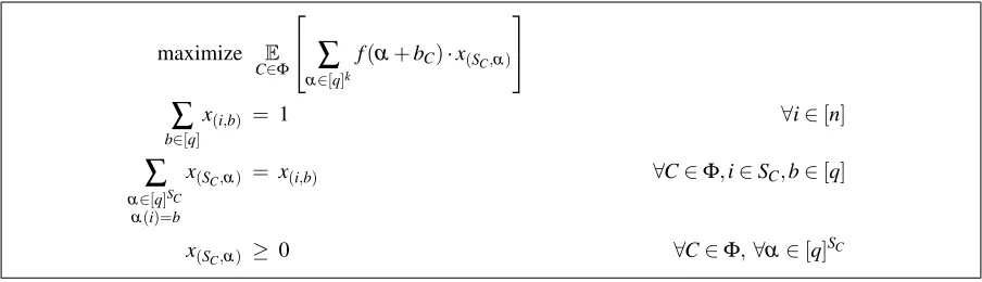
The basic LP relaxation is a reduced form of the above relaxation where only those variablesx₍S,α)are included for whichS=SCis the set of CSP variables for some constraintC. The consistency constraints

are included only for singleton subsets of the setsSC. We note here that for any feasible solution to

basic LP relaxation, the local distributions{x₍S,α)}assign the same value to the repeated variables of a constraint. Note that the all the constraints for the basic LP are implied by the relaxation obtained by levelkof the Sherali–Adams hierarchy.

For an LP/SDP relaxation ofMAX k-CSPq, and for a given instanceΦof the problem, we denote by

maximize E C∈Φ





∑

α∈[q]k

f(α+bC)·x(SC,α)





∑

b∈[q]

x(i,b) = 1 ∀i∈[n]

∑

α∈[q]SC

α(i)=b

x(SC,α) = x(i,b) ∀C∈Φ,i∈SC,b∈[q]

x_(SC,α) ≥ 0 ∀C∈Φ,∀α∈[q]SC

Figure 2: Basic LP relaxation forMAX k-CSPq(f).

2.3 Hypergraphs

An instanceΦofMAX k-CSPdefines a natural associated hypergraphH= (V,E)withV being the set of variables inΦandEcontaining one hyperedge for every constraintC∈Φ. We remind the reader of the familiar notions of degree, paths, and cycles for the case of hypergraphs:

Definition 2.2. LetH= (V,E)be a hypergraph.

• For a vertexv∈V, thedegreeof the vertexvis defined to be the number of distinct hyperedges containing it.

• Asimple pathPis a finite alternate sequence of distinct vertices and distinct edges starting and ending at vertices, i. e.,P=v1,e1,v2, . . . ,v`,e`,v`+1, wherevi∈V ∀i∈[`+1]andei∈E∀i∈[`].

Furthermore,ei containsvi,vi+1 for eachi. Here`is called thelengthof the pathP. All paths

discussed in this paper will be simple paths.

• A sequence C= (v₁,e₁,v₂, . . . ,v_{`</sub>,e<sub>`},v₁) is called a cycle of length ` if the initial segment

v1,e1, . . . ,v` is a (simple) path, e` 6=ei and |ei|>1 for all i∈[`], andv1∈e`. We note that

we don’t include hyperedges with only one vertex towards forming cycles. For a pathP(or cycle

C), we use V(P)(or V(C)) to denote the set of all the vertices that occur in the edges, i. e., the set

{v : (∃i∈[h])(v∈ei)}, wheree1, . . . ,ehare the hyperedges included inP(orC). For a pathP,|P|

denotes the number of hyperedges on the pathP.

• For a given hypergraphH, the length of the smallest cycle inHis called thegirthofH.

To observe the difference the notions of cycle in graphs and hypergraphs, it is instructive to consider the following example: letu,vbe two distinct vertices in ak-uniform hypergraph fork≥3, and lete1,e2

be two distinct hyperedges both containinguandv. Thenu,e1,v,e2,uis a cycle of length 2, which cannot

occur in a graph.

Definition 2.3. For a given hypergraphH and R∈_N, and a setS⊆V(H), we denote by clR(S) the R-closureofSobtained by adding all the vertices in all the paths of length at mostRconnecting two vertices ofS, i. e.,

clR(S) = S∪



    

[

P:Pis a path inH Pconnectsu,v∈S

|P|≤R

V(P)



    

.

For ease of notation, we use cl(S)to denote cl1(S).

3

Properties of random hypergraphs

In this section we collect various properties of the hypergraphs corresponding to our integrality gap instances. The gap instances we generate contain several disjoint collections of variables. Each constraint in the instance has a specified “type”, which specifies which of the collections each of the participating

kvariables much be sampled from. The constraint is generated by randomly sampling each of thek

variables, from the collections specified by its type. This is captured by the generative model described below.

In the model below and in the construction of the gap instance, the parametern0should be thought

of as constant, while the parametersnandmshould be though of a growing to infinity. We will choose

m=γ·nforγ=Ok,q(1).

Definition 3.1. Letn0,k∈Nwithk≥2. Letm,n∈Nand letΓbe a distribution on[n0]k. We define

a distribution Hk(m,n,n0,Γ) on n0-partite hypergraphs on N =n0·n vertices, divided into n0 sets, X1, . . . ,Xn0, of sizeneach. EachH∈Supp(Hk(m,n,n0,Γ))hasmedges and each edge has at mostk vertices. A random hypergraphH∼Hk(m,n,n0,Γ)is generated by samplingmrandom hyperedges

independently as follows:

• Sample a random type(i1, . . . ,ik)∈[n0]kfrom the distributionΓ. • For all distinctij, samplevij independently and uniformly fromXij.

• Add the edgeei={vi1, . . . ,vik}toH.

Note that as specified above, the model may generate a multi-hypergraph. However, the number of such repeated edges is likely to be small, and we will bound these, and in fact the number of cycles of size o(logn)inLemma A.2.

We will study the following metrics (similar to the ones defined in [11]):

Definition 3.2. Given a hypergraphHwith vertex setV, we define two metricsd_µH(·,·),ρ_µH(·,·)onV as

dH_µ(u,v) := 1−(1−µ)2·dH(u,v) and ρ_µH(u,v) :=

s

2·dH

µ(u,v) +µ

1+µ ,

We primarily need the local`2-embeddability of the metricρ_µH. The following theorem captures

various properties of random hypergraphs required for our construction. The proof of the theorem heavily uses results proved in [3] and [9] and we defer the details toAppendix A.

Theorem 3.3. LetH0∼Hk(m,n,n0,Γ)withm=γ·nedges and letε >0. Then for large enoughn,

with high probability (at least 1−ε, over the choice ofH0), there existδ>0, constantc=c(k,γ,n0,ε), θ=θ(k,γ,n0,ε)and a subhypergraphH⊂H0withV(H) =V(H0)satisfying the following:

• H has girthg≥δ·logn.

• |E(H0)\E(H)| ≤ε·m.

• For allt≤nθ_{, for}

µ≥c·(logt+log logn)/logn, for allS⊆V(H0)with|S| ≤t, the metricρ_µH

restricted toSis isometrically embeddable into the unit sphere in`2.

4

Decompositions of hypergraphs from local geometry

We will construct the Sherali–Adams solution by partitioning the given subset of vertices into trees, and then creating a natural distribution over satisfying assignments on trees. We define below the kind of partitions we need.

Definition 4.1(Consistent Partitioning Scheme). Let X be a finite set. For a set S, let PS denote a

distribution over partitions ofS. ForT ⊆S, letPS|T be the distribution over partitions ofT obtained by

restricting the partitions inPSto the setT. We say that a collection of distributions{PS}_|S|≤t forms a

consistent partitioning scheme of ordert, if

∀S⊆X,|S| ≤t and ∀T ⊆S PT =PS|T.

In addition to being consistent as described above, we also require the distributions to have small probability of cutting the hyperedges for the hypergraphs corresponding to our CSP instances. We define this property below.

Definition 4.2. Let H= (V,E) be a hypergraph with each hyperedge having at mostk vertices. Let

{PS}_|S|≤t be a consistent partitioning scheme of ordert for the vertex setV, witht≥k. We say the scheme{PS}|S|≤t isε-sparseforHif

∀e∈E _P P∼_Pe

[eis cut byP] ≤ ε.

In this section, we will prove that the hypergraphs arising from random CSP instances admit sparse and consistent partitioning schemes. Recall that for a hypergraphH, we define (Definition 3.2) the metrics

d_µHandρ_µHas:

dH_µ(u,v) := 1−(1−µ)2·dH(u,v) _{and ρ}H

µ(u,v) :=

s

2·dH

µ(u,v) +µ

Lemma 4.3. Let H= (V,E) be hypergraph with each hyperedge containing at most k vertices and letρ_µH be the metric as defined above. Further, let H be such that for all sets S⊆V with|S| ≤t, the metric induced onρ_µH on S is isometrically embeddable into`2. Then, there existsε≤10k·

√

µ·t and

∆H=O(1/µ) such that H admits an ε-sparse consistent partitioning scheme of order t, with each partition consisting of clusters of diameter at most∆Hin H.

We use the following result of Charikar et al. [8] which shows that low-dimensional metrics have good

separating decompositionswith bounded diameter, i. e., decompositions which have a small probability of separating points at a small distance.

Theorem 4.4([8]). Let W be a finite collection of points inRd and let∆>0be given. Then there exists a distributionPover partitions of W such that

- ∀P∈Supp(P), each cluster in P has`2diameter at most∆, and

- for all x,y∈W

P

P∼_P[P separates x and y] ≤ 2

√

d·kx−yk2

∆ .

We also need the observation that the partitions produced by the above theorem are consistent, assuming the setS considered above lies in a fixed bounded set (using a trivial modification of the procedure in [8]). For the sequel, we useB(x,δ)to denote the`2ball aroundxof radiusδ andBH(u,r)

to denote a ball of radiusraround a vertexu∈V(H). Thus,

B(x,δ) := {y | kx−yk₂≤δ} and BH(u,r) := {v∈V | dH(u,v)≤r}.

The ballsB(S,δ)andBH(S,r)are defined similarly.

Claim 4.5. Let S and T be sets such that T ⊆S. Let WS={wu}_u∈Sand WT={w0u}u∈T be`2-embeddings of S and T satisfyingφ(WT)⊆WS⊆B(0,R0)⊂Rd, for some unitary transformationφ and R0>0. Let PSandPT be distributions over partitions of S and T respectively, induced by partitions on WSand WT as given byTheorem 4.4. Then

PS|T = PT.

Proof. The claim follows simply by considering (a trivial modification of) the algorithm of [8]. For a given setW and a parameter∆, they produce a partition using the following procedure:

• LetW0=W.

• Repeat untilW0=/0

– Pick a random pointxinB(W,∆/2)according to the Haar measure. LetCx=B(x,∆/2)∩W0.

[8] show that the above procedure produces a distribution over partitions satisfying the conditions in

Theorem 4.4. We simply modify the procedure to sample a random pointxinB(0,R0+∆/2)instead of B(W,∆/2). This does not affect the separation probability of any two points, since the only non-empty clusters are still produced by the points inB(S,∆/2). SinceR0+∆<∞, the above procedure almost surely terminates in finitely many steps.

LetPbe a partition ofSproduced by the above procedure when applied to the point setWS, and

letP0 be a random partition produced when applied to the point setφ(WT). It is easy to see from the

above procedure that the distributionPT is invariant under a unitary transformation ofWT. By coupling

the random choice of a point inB(0,R0+∆/2) chosen at each step in the procedures applied toWS

andφ(WT)⊆WS, we get that P(T) =P0, i. e., the partitionPrestricted toT equalsP0. Thus, we get PS|T=PT.

We can use the above to proveLemma 4.3.

Proof ofLemma 4.3. Given a setS, letWSbe an`2embedding of the metricρµ restricted toS. Since |S| ≤t, we can assumeWS∈Rt. We apply partitioning procedure of Charikar et al. fromTheorem 4.4 with∆=1/2. From the definition of the metricρ_µH, we get that there exists a∆H=O(1/µ)such that

ρuH,v≤1/2 =⇒ dH(u,v)≤∆H.

Moreover, foru,vcontained in an edgee, we have thatρµ(u,v)≤ √

5µ and hence the probability thatu

andvare separated is at most 10√µ·t. Thus, the probability that any vertex ineis separated fromuis at

most 10k·√µ·t– asecontains at mostkvertices.

Finally, for anyS⊆T, ifWSandWT denote the corresponding`2embeddings, by the rigidity of`2

we have that forφ(WT)⊆WSfor some unitary transformationφ. Thus, byClaim 4.5, we get that this is a

consistent partitioning scheme of ordert.

5

The Sherali–Adams integrality gaps construction

5.1 Integrality gaps from the basic LP

Recall that the basic LP relaxation forMAX k-CSPq(f) as given inFigure 2. In this section, we will

proveTheorem 1.1. We recall the statement below. Theorem 1.1. Let f :[q]k_{→ {0,1}be any predicate. Let}

Φ0be a(c,s)-integrality gap instance for basic

LP relaxation ofMAX k-CSP(f). Then for everyε >0, there exists cε >0 such that for infinitely

manyN∈_N, there exist(c−ε,s+ε)-integrality gap instances of sizeNfor the LP relaxation given by

cε·logN/log logNlevels of the Sherali–Adams hierarchy.

LetΦ0be a(c,s)integrality gap instance for the basic LP relaxation forMAX k-CSPq(f) withn0

Given: A(c,s)gap instanceΦ0onn0variables, for the basic LP.

Output: An instanceΦwithN=n·n0variables andmconstraints.

The variables are divided inton0 sets,X1, . . . ,Xn0, one for each variable inΦ0. We generatem constraints independently at random as follows:

1. Sample a random constraintC0∼Φ0. Let xC0 = (i1, . . . ,ik)⊆[n0]denote the multi-set of variables in this constraint.

2. For each distinctijfor j∈[k], sample a random variablexij ∈Xij. We note that ifij=ij0 then

we setXij =Xij0.

3. Add the constraint f((xi1, . . . ,xik) +bC0)to the instanceΦ.

Figure 3: Construction of the gap instanceΦ.

Soundness

We first prove that no assignment satisfies more thans+ε fraction of constraints for the above instance.

Lemma 5.1. For everyε >0, there exists γ =γ(ε,n0,q) such that for an instanceΦ generated by choosing at leastγ·n constraints independently at random as above, we have with probability 1−

exp(−Ω(n)),OPT(Φ)<s+ε.

Proof. Fix an assignmentσ∈[q]N_{. We will first consider}

E[satΦ(σ)]for a randomly generatedΦas above.

E Φ

[satΦ(σ)] = E

C0∈Φ0 E (xi1,...,xik)

f(σ(xi1) +bi1, . . . ,σ(xik) +bik)

= E

C0∈Φ0 E

Z1,...Zn₀

[f(ZC0+bC0)],

where for eachi∈[n0],Ziis an independent random variable with the distribution

P[Zi=b] := E

x∈Xi

1{σ(x)=b}

,

andZC0 denotes the collection of variables in the constraintC0, i. e.,

ZC0 = {Zi}i∈SC₀.

Thus, the random variablesZ1, . . . ,Zn0 define a random assignment to the variables inΦ0, which gives, for anyσ

E Φ

[satΦ(σ)] = E

C0∈Φ0 E

Z1,...Zn₀

[f(ZC0+bC0)] < s.

Consider a randomly added constraintCto the instanceΦ. We have that P[C(σ) =1] = E

Φ

for any fixedσ over random choice of the constraintC. Thus, for an instanceΦwithmindependently and randomly generated constraints, we have

P Φ

[satΦ(σ) ≥ s+ε] ≤ P Φ

satΦ(σ) ≥ E Φ

[satΦ(σ)] +ε

= P Φ

E

C∈Φ

1{C(σ)=1}

≥ _E

Φ

[satΦ(σ)] +ε

≤ exp −Ω(ε2·m)

.

Taking a union bound over all assignments, we get

P Φ

[∃σ satΦ(σ) ≥ s+ε] ≤ qn·n0·exp −ε2·m,

which is at most exp(−Ω(n))form=O(((logq)/ε2)·n·n0).

Completeness

To prove the completeness, we first observe that the instanceΦas constructed above is also a gap instance for the basic LP. We will then “boost” this hardness to many levels of the Sherali–Adams hierarchy. Lemma 5.2. For everyε>0, there existsγ=γ(ε)such that for an instanceΦgenerated by choosing at

leastγ·n constraints independently at random as above, with probability1−exp(−Ω(n))there exist

distributionsDSC over[q]

SC_{for each C}∈_{Φ, and distributions}D

iover[q]for each variable i∈[n·n0], satisfying:

- For all C∈Φand all i∈SC,DSC|{i}=Di;

- The distributions satisfy _E C∈Φ_α∼E_DSC

[f(α+bC)] ≥ c−

ε

10.

Proof. For eachC0∈Φ0and each j∈[n0], letD(S0C)0 andD (0)

j denote the basic LP solution satisfying D(0)

SC₀|j = D

(0)

j ∀C0∈Φ0∀j∈SC0 and E

C0∈Φ0 E

α∼D(_SC0)

0

[f(α+bC0)] ≥ c.

Each constraintC∈Φis sampled according to some constraintC0∈Φ0, and we takeDSC :=D

(0)

SC0 for the corresponding constraintC0∈Φ0. Also, each variablexifori∈[n0·n], belongs to one of the setsXj

for j∈[n0], and we takeDi:=D(j0)for the corresponding j∈[n0].

The consistency of the distributions follows immediately from the construction of the instanceΦ. LetC∈Φbe any constraint and letC0be the corresponding constraint inΦ0. IfxC0 = (j1, . . . ,jk), then

xC= (i1, . . . ,ik)where eachir∈ {jr} ×[n]for all distinct jr. Thus, for anyr∈[k], DSC|ir = D

(0)

SC₀|jr = D

(0)

We note that the repeated variables inxC0 gets thesame value under the basic LP solutionD (0)

SC₀ and

therefore the same is true forDSC. To bound the objective value, we again consider its expectation over a

randomly generated instanceΦ. LetCbe a random constraint added toΦ. Then, if we defineDSC as

above for this constraint, we have

E

C_α∈E_D

SC

[f(α+bC)] = E

C0∈Φ0 E

α∼D(0)

[f(α+bC0)] ≥ c.

Thus, the expected contribution of each constraint is at leastc. The probability that the average ofm

constraints deviates by at leastε/10 from the expectation, is at most exp −Ω(ε2·m). There exists γ=O(1/ε2)such that form≥γ·n, the probability is at most exp(−Ω(n)).

To construct local distributions for the Sherali–Adams hierarchy, we will consider (a slight modifica-tion of) the hypergraphHcorresponding to the instanceΦ. We first show that distributions on hyperedges of this hypergraph can be consistently propagated in a tree, provided they agree on intersecting vertices.

For a setU ⊆V(H) in a hypergraphH, recall that cl(U)includes all paths of lengths at most 1 between any two vertices inU. Thus,E(cl(U)) ={e∈E | |e∩U| ≥2}. Note thatLemma 5.2implies that hyperedges forming a tree inHsatisfy the hypothesis ofLemma 5.3below.

Lemma 5.3. Let H= (V,E)be a hypergraph. Let U⊆V be such that the set of hyperedges E(cl(U))

form a tree. For each e∈E(cl(U)), letDe be a distribution on [q]e such that for any u∈U and e1,e2∈E(cl(U))such that e1∩e2={u}, we haveDe1|u=De2|u=Du. Then,

- there exists a distributionDU on[q]Usuch thatDU|e∩U =De|e∩Ufor all e∈E(U);

- if U0⊆U is such that the hyperedges in E(cl(U0))form a subtree of E(cl(U)), thenDU|U0=D_U0.

Proof. We define the distribution by starting with an arbitrary hyperedge and traversing the tree in an arbitrary order. Lete1, . . . ,erbe a traversal of the hyperedges inE(cl(U))such that for alli,

[

j<i ej

!

∩ei

= 1.

LetU0=Sj<iej be the set of vertices for which we have already sampled an assignment and leteibe the

next hyperedge in the traversal, withubeing the unique vertex inei∩U0. We sample an assignment to

the vertices ine, conditioned on the value for the vertexu. Formally, we extend the distributionDU0 to

U0∪eby taking, for anyα∈[q]U0∪e

DU0∪e(α) = DU0(α(U0))·

De(α(e)) De|u(α(u))

= DU0(α(U0))·

De(α(e)) Du(α(u))

.

The above process defines a distributionDcl(U)on cl(U), with

Dcl(U)(α) =

∏e∈E(U)De(α(e))

∏u∈cl(U) Du(α(u))deg(u)−1

In the above expression, we use deg(u)to denote the degree of vertexuin tree formed by the hyperedges in

E(cl(U)), i. e., deg(u) =|{e∈E(cl(U))|u∈e}|. We then define the distributionDUas the marginalized

distributionDcl(U)|U, i. e.,

DU(α) =

∑

β(U)=α

Dcl(U)(β).

Note that the distributionDcl(U)and hence also the distributionDUare independent of the order in which

we traverse the hyperedges inE(cl(U)). Also, since the above process samples each hyperedge according to the distributionDe, we have that for anye∈E(U),Dcl(U)|e=De. Thus, also for anye∈E(U),

DU|e∩U = De|e∩U.

LetU0⊆U be any set such thatE(cl(U0))forms a subtree ofE(cl(U)). Then there exists a traversal

e₁, . . . ,er, andi∈[r]such thatej∈E(cl(U0))∀j≤iandej∈/E(cl(U0))∀j>i. However, the distribution

defined by the partial traversale1, . . . ,eiis preciselyDcl(U0₎. Thus, we get that Dcl(U)|cl(U0₎ = D_cl(U0₎

which impliesDU|U0 =D_U0.

We can now prove the completeness for our construction using consistent decompositions.

Lemma 5.4. Let ε >0 and let Φ be a random instance of MAX k-CSPq ( f ) generated by choos-ing γ·n constraints independently at random as above, for large enough n. Then, there is a t =

Ωε,k,n0(logn/log logn), such that with probability1−ε over the choice ofΦ, there exist distributions

{DS}_|S|≤t satisfying:

- For all S⊆V with|S| ≤t,DSis a distribution on[q]S.

- For all T ⊆S⊆V with|S| ≤t,DS|T=DT.

- The distributions satisfy

E

C∈Φ αC∼ED_SC

[f(αC+bC)] ≥ c−ε.

Proof. ByTheorem 3.3, we know that there existsδ such that with probability 1−ε/4, after removing

a set of constraintsCB of size at most(ε/4)·m, we can assume that the remaining instance has girth

at least g=δ·logn. Also, there exist θ,c>0 such that for all large enoughn, for all t≤nθ, the

metricρ_µHrestricted to any setSof size at mosttembeds isometrically into the unit sphere in`2, for all

µ≥c·(logt+log logn)/logn.

We chooseµ =2c·log logn/lognandt=ε2/(400k2·µ)so that µ ≥ c·logt+log logn

logn and

√

µ·t ≤ ε

20k.

Thus, byLemma 4.3,Hadmits an(ε/2)-sparse partitioning scheme of ordertwith each cluster in the

Given a setS, the distributionDSis a convex combination of several distributionsDS,P, corresponding

to different partitionsPsampled fromPS. We describe the distributionDSby giving the procedure to

sample anα∈[q]S. Given the setSwith|S|:≤t

- Sample a partitionP= (U₁, . . . ,Ur)from the distributionPS.

- For each setUi, consider the set C(Ui) obtained by including the vertices contained in all the

hyperedges in the shortest path between allu,v∈Ui. Note that sinceUi has diameter at most

∆H in H, C(Ui) is connected and in fact C(Ui) =cl∆H(Ui). Also, since the each vertex in an

included path is within distance at most∆H/2 of an end-point, andUi has diameter at most∆H, we

know that the diameter ofC(Ui)is at most 2·∆H. Hence,C(Ui)is a tree. Finally, we must have

cl(C(Ui)) = C(Ui)since any additional path of length 1 would create a cycle of length at most

2·∆H+1.

Thus, byLemma 5.2andLemma 5.3(with probability at least 1−ε/4) there exists a distribution

DC(Ui)for eachUi, satisfying

D_C(Ui)|e = De

for alle∈E(C(Ui)). Here,Deare the distributions given byLemma 5.2, which form a solution to

the basic LP forΦ, with value at leastc−ε/4. For eachUi, define the distribution D0

Ui := DC(Ui)|Ui.

- Sampleα∈[q]S_{according to the distribution}

DS,P := DU01× · · · ×D 0

Ur.

Thus, we have

DS := E

P=(U1,...,Ur)∼PS

"

r

∏

D0

Ui

#

,

where the distributionsD0_U

i are defined as above.

We first prove the distributions are consistent on intersections, i. e.,DS|T=DT for anyT ⊆S. Note

that byLemma 4.3, the distributionsPSandPT satisfyPS|T =PT. Each partition(U1, . . . ,Ur)ofSalso

produces a partitionT. For ease of notation, we assume that the first (say)r0clusters have non-empty intersection withT. LetVi=Ui∩T for 1≤i≤r0(Vi= /0 fori>r0). Then, we have

DS|T = E

P=(U1,...,Ur)∼PS

"

r

∏

D0

Ui|Vi

#

= E

P=(U1,...,Ur)∼PS

"

r0

∏

D_C(Ui)|Vi

#

= E

P=(U1,...,Ur)∼PS

"

r0

∏

D_C(Vi)|Vi

#

= E

P0_=(V

1,...,Vr0)∼PT

"

r0

∏

D_C(Vi)|Vi

#

The second to last equality above uses the fact thatC(Vi)is a subtree ofC(Ui)and thus DC(Ui)|C(Vi) = DC(Vi)

byLemma 5.3. The last equality uses the fact thatPS|T =PT byLemma 4.3.

We now argue that the LP solution corresponding to the above distributions{DS}|S|≤t has value at

leastc−ε. Recall that the value of the LP solution is given by E

C∈Φ α∼ED_SC

[f(α+bC)].

Consider any constraintC in Φ, with the corresponding set of variables SC and the corresponding

hyperedgee. When defining the distributionDSC, we will partitionSCaccording to the distributionPSC.

ByLemma 4.3and our choice of parameters

P

P∼P_SC[SCis separated byP] ≤ 10k·

√

µ·t ≤ ε

2.

For a constraint set which is not in the deleted setCB, if the hyperedgeecorresponding to the constraint Cis not split by a partitionPsampled according toPSC, then byLemma 5.3

DSC,P = DSC.

Here,DSCis the distribution given byLemma 5.2. Since f is Boolean, we have that forC∈/CB,

E

α∼D_SC

[f(α+bC)] ≥ E

α∼D_SC

[f(α+bC)]−

ε

2. UsingLemma 5.2again, we get

E

C∼Φ α∼ED_SC

[f(α+bC)] ≥ E

C∼Φ

"

1−_1{C∈CB}

· _E

α∼D_SC

[f(α+bC)]−

ε

2

!#

≥ _E

C∼Φ_α∼ED_SC

[f(α+bC)]−

ε

2−CE∼Φ

1{C∈CB}

≥ c−ε

4−

ε

2−

ε

4

≥ c−ε,

where the penultimate inequality uses the fact that the fraction of constraints in the initially deleted setCB

is at mostε/4 (for large enoughn).

5.2 Integrality gaps for resistant predicates

Let f :{0,1}k_{→ {0,1}be a Boolean predicate and let}

ρ(f) =f−1(1)

/2kbe the fractions of satisfying

assignments to f. Then f is approximation resistant if it is hard to distinguish theMAX-CSPinstances on

In [19] the authors introduce the notion ofvanishing measure(on a polytope defined by f) and use it to characterize a variant of approximation resistance, called strong approximation resistance, assuming the Unique Games conjecture. They also gave aweakernotion of vanishing measures, which they used to characterize strong approximation resistance for LP hierarchies. In particular, they proved that when the condition in their characterization is satisfied, there exists a(1−o(1),ρ(f) +o(1))-integrality gap for O(log logn)levels of Sherali–Adams hierarchy for predicates f. Here, we show that usingTheorem 1.1, their result can be simplified and strengthened1to O(logn/log logn)levels.

Let us first recall some useful notation defined by Khot et al. [19] before we define the notion of vanishing measure:

Definition 5.5. For a predicate f :{0,1}k_{→ {0,1}, letC(f)be the convex polytope offirstmoments}

(biases) of distributions supported on satisfying assignments of f, i. e.,

C(f) := nζ ∈Rk

∀i∈[k],ζi=_αE_∼ν[(−1)

αi_{], Supp(ν)⊆ f}−1₍₁₎

o

.

For a measureΛonC(f),S⊆[k],b∈ {0,1}Sand permutationπ:S→S, letΛS,π,bdenote the induced

measure onRSby considering vectors with coordinates

n

(−1)bπ(i)_·ζ π(i)

o

i∈S,

whereζ ∼Λ.

We recall below the definition of vanishing measure for LPs from [19] (see Definition 1.3) :

Definition 5.6. A measureΛonC(f)is calledvanishing(for LPs) if for every 1≤t≤k, the following signed measure

E

|S|=t π:SE→Sb∈{E0,1}t

"

t

∏

(−1)bi

!

·_fˆ_(S)·ΛS,π,b

#

is identically 0. We say f has a vanishing measure if there exists a vanishing measureΛonC(f). In particular, they prove the following theorem:

Theorem 5.7. Let f :{0,1}k_{→ {0,1}be a k-ary Boolean predicate that has a vanishing measure. Then} for everyε>0, there is a constant cε>0such that for infinitely many N∈N, there exists an instanceΦ ofMAX k-CSP(f)on N variables satisfying the following:

• OPT(Φ) ≤ ρ(f) +ε.

• The optimum for the LP relaxation given by c_ε·log logN levels of Sherali–Adams hierarchy has FRAC(Φ) ≥ 1−O(k·√ε).

1_{The LP integrality gap result of Khot et al. is in fact slightly stronger than stated above. They show that LP value is at least}

Combining this with ourTheorem 1.1already gives us the following stronger result:

Corollary 5.8. Let f :{0,1}k_{→ {0,1}be a k-ary Boolean predicate that has a vanishing measure. Then} for everyε>0, there is a constant cε >0such that for infinitely may N∈N, there exists an instanceΦ ofMAX k-CSP(f)on N variables satisfying the following:

• All integral assignment ofΦsatisfies at mostρ(f) +ε fraction of constraints.

• The LP relaxation given by cε·logN/log logN levels of Sherali–Adams hierarchy has

FRAC(Φ) ≥ 1−O(k√ε).

However, note that to applyTheorem 1.1, one only needs a gap for the basic LP, which is much weaker requirement than the O(log logN)-level gap given byTheorem 5.7. We observe below that the gap for the basic LP follows very simply from the construction by Khot et al. [19]. One can then directly use this gap for applyingTheorem 1.1instead of going throughTheorem 5.7.

Khot et al. [19] use the probabilistic construction given inFigure 4, for a givenε>0. The construction actually requiresΛto be a vanishing measure over the polytopeCδ(f):= (1−δ)·C(f), forδ =

√

ε.

However, sinceC_δ(f)is simply a scaling ofC(f), a vanishing measure overC(f)also gives a vanishing measure overCδ(f). Note that eachζ0∈C(f)corresponds to a distribution ν0 supported in f

−1_(1).

For eachζ ∈Cδ, letζ0=ζ/(1−δ)be the point inC(f)with distributionν0. Then the distribution

ν= (1−δ)·ν0+δ·Uk(whereUk denotes the uniform distribution on{0,1}k) satisfies ∀i∈[k] E

α∼ν[(

−1)αi_{] =}

ζi.

Letn0=d1/εe. Partition the interval[0,1]inton0+1 disjoint intervalsI0,I1, . . . ,In0 whereI0={0} andIi= ((i−1)/n0,i/n0]for 1≤i≤n0. For each intervalIi, letXibe a collection ofnvariables

(disjoint from allXjfor j6=i).

Generatemconstraints independently according to the following procedure:

• Sampleζ ∼Λ.

• For each j∈[k], letij be the index of the interval which contains|ζ(j)|. Sample uniformly a

variableyj from the setXj.

• Ifζ(j)<0, then negateyj. Ifζ(j) =0, then negateyj with probability 1/2. • Introduce the constraint f on the sampledk-tuple of literals.

Figure 4: Sherali–Adams integrality gap instance for vanishing measure.

They show for a sufficiently large constantγ, an instanceΦwithm=γ·nconstraints satisfies with high probability, that for all assignmentsσ,|satΦ(σ)−ρ(f)| ≤ε(see Lemma 4.4 in [19]). The proof is

Additionally, we need the following claim from [19] (see Claim 4.7 there), which allows one to “round” coordinates of the vectorsζ∈C_δ(f)to the end-points of the intervalsI0, . . . ,In0. This ensures that any two variables in the same collectionXihave the same bias. The proof of the claim follows simply

from a hybrid argument. We include it in the appendix for completeness.

Claim 5.9. Letζ ∈C_δ(f)and letνbe the corresponding distribution supported in f−1(1)such that for all i∈[k], we have

ζi = E

α∼ν[(

−1)αi_].

Let t1, . . . ,tk∈[0,1]be such that for all i∈[k],|ti− |ζi|| ≤εforε<δ/2. Then there exists a distribution ν0 on{0,1}ksuch that

ν−ν0

1 = O(k·(ε/δ)) and ∀i∈[k], _αE_∼ν0[(−1)

αi_{] = sign(ζ}

i)·ti.

Proof. Letrj=sign(ζj)·tjbe the desired bias of the j-th coordinate. Then,

ζ(j)−rj

≤εfor all j∈[k].

We construct a sequence of distributionsν0, . . . ,νk such thatν0=ν andνk=ν0. In ¯νj, the biases are

(r1, . . . ,rj,ζj+1, . . . ,ζk).

The biases inν0satisfy the above by definition. We obtain ¯νj from ¯νj−1as,

νj = (1−τj)·νj−1+τj·Dj,

whereDjis the distribution in which all bits, except for the j-th one, are sampled independently according

to their biases in ¯νj−1. For the j-th bit, we fix it to sign(rj−ζj)(ifrj−ζ(j) =0, we can simply proceed

with ¯νj=ν¯j−1). The biases for all except for the j-th bit are unchanged. For the j-th bit, the bias now

becomesrjif

rj= (1−τj)·ζj+τj·sign(rj−ζj) =⇒ τj·(sign(rj−ζj)−rj) = (1−τj)·(rj−ζj).

Sinceζ∈C_δ(f), we know thatsign(rj−ζ(j))−rj

≥δ/2. Also,

rj−ζ(j)

≤ε by assumption. Thus,

we can chooseτj=O(ε/δ)which gives that

ν¯j−ν¯j−1

1=O(ε/δ). The final bound then follows by

triangle inequality.

We can now use the above to give a simplified proof ofCorollary 5.8.

Proof ofCorollary 5.8. Here we exhibit a solution of the basic LP (Figure 2) for the instance given in

Figure 4. For each variableyjcoming from the setXjfor j∈ {0,1, . . . ,n0}, we fix the biastjof the variable

to be the rightmost point of the intervalIj, i. e., fixx(yj,−1)= (1−j/n0)/2 andx(yj,1)= (1+j/n0)/2.

For each constraintC of the form f(yi1+b1, . . . ,yik+bk), let ζ(C)∈Cδ(f) be the point used to

generate it, and letν(C)denote the corresponding distribution on{0,1}k. ByClaim 5.9, there exists a

distributionν0(C)such thatkν(C)−ν0(C)k₁=O(k·ε/δ)and such that the biases of theliteralssatisfy

E

α∼ν0(C)[(−1)

αj_{] = sign(}

ζj)·tij,

wheretij denotes the bias for the interval to whichyij belongs. Whentij 6=0, we negate a variable only

when sign(ζj)<0. Thus, we have

E

α∼ν0(C)

h

(−1)αj+bj

i

which is consistent with the bias given by the singleton variablesx_(y

i j,1)andx(yi j,−1). We thus define the

local distribution on the setSCas

DSC(α) = (ν

0_(C))(

α+bC).

For allC∈Φ, sinceζ(C)∈Cδ(f), we have that

E

α∼ν(C)[f(α)] ≥ 1−δ. Also, sincekν(C)−ν0(C)k₁=O(k·ε/δ), we get that

E

α∼ν0(C)[

f(α)] ≥ 1−δ−O(k·ε/δ).

Thus, we have for allC∈Φ,

E

α∼D_SC

[f(α+bC)] ≥ 1−δ−O(k·ε/δ).

Takingδ =

√

εproves the claim.

5.3 Lower bounds for LP extended formulations

A connection between LP integrality gaps for the Sherali–Adams hierarchy, and lower bounds on the size of LP extended formulations, was first established by Chan et al. [7] and later improved by Kothari et al. [21]. In [21], the authors proved the following:

Theorem 5.10 ([21], Theorem1.2). There exist constants 0<h<H such that the following holds. Consider a function g:N→N. Suppose that the g(n)-level Sherali–Adams relaxation for a CSP cannot achieve a(c,s)-approximation on instances on n variables. Then, no LP extended formulation (of the original LP) of size at most nh·g(n)can achieve a(c,s)-approximation for the CSP on nH variables.

CombiningTheorem 1.1withTheorem 5.10yields (withg(N):=c_ε·logN/log logN) we get the following corollary.

Corollary 1.2. Let f :[q]→ {0,1}be any predicate. LetΦ0be a(c,s)-integrality gap instance for basic LP relaxation ofMAX k-CSP( f ). Then for everyε>0, there exists c0_ε>0such that for infinitely many

N∈_N, there exist(c−ε,s+ε)-integrality gap instances of size N, for every linear extended formulation

of size at most Nc0ε·logN/log logN.

6

Conclusions and open problems

This work shows a dichotomy result for approximating CSPs using linear programs, proving that if a(c,s) approximation is not achievable using the basic LP, then for everyε>0,(c−ε,s+ε)approximation

is not achievable using Oε(logn/(log logn))levels of the Sherali–Adams hierarchy. A natural open

this would also show that even exponential-size LP extended formulations are at most as strong as the basic LP.

As mentioned in the paper, the current limitation on the number of levels in our result, comes from the consistency requirement of the low-diameter decompositions. Given ad-dimensional`2embedding of the

restriction of the metricρ_µHto a set of verticesS, the fraction of edges cut by the decomposition procedure of [8] grows as√d. Our current proof only uses the trivial bound that when|S|=t, the metric admits a

t-dimensional`2embedding. Even though for a single setS, this bound can be improved to O(logt)at

the cost of slight errors in the distances (using randomized dimension reduction), we do not know how to do thisconsistentlyacross various setsS. In particular, since we want to always obtain low-diameter components, we may need to reject a small fraction of dimension reduction maps forS, if they shrink the distances too much. However, such maps may not necessarily be rejected when consideringT ⊆S, which can violate the consistency requirementPS|T = PT. Understanding how and when randomized

dimension reduction can be combined with the consistency requirement is an intriguing question which may also be useful in other applications.

Acknowledgements

We thank Chandra Chekuri, Subhash Khot and Yury Makarychev for helpful discussions, and Rishi Saket for pointers to references. We are also grateful to the CCC 2017 reviewers, and the ToC referees and editors, for numerous suggestions to improve the presentation of this paper. This research was supported by the National Science Foundation under award number CCF-1254044.

A

Local

`

-embeddability of the Metric

ρ

The goal of this section is to prove the following result about the local`2-embeddability of the metricρµH.

Theorem 3.3. LetH0∼Hk(m,n,n0,Γ)withm=γ·nedges and letε >0. Then for large enoughn,

with high probability (at least 1−ε, over the choice ofH0), there existδ>0, constantc=c(k,γ,n0,ε), θ=θ(k,γ,n0,ε)and a subhypergraphH⊂H0withV(H) =V(H0)satisfying the following:

• H has girthg≥δ·logn.

• |E(H0)\E(H)| ≤ε·m.

• For allt≤nθ_{, for}

µ≥c·(logt+log logn)/logn, for allS⊆V(H0)with|S| ≤t, the metricρ_µH

restricted toSis isometrically embeddable into the unit sphere in`2.

To prove the above theorem, we will use the local structure of random hypergraphs. We first prove that with high probability for random hypergraphs (sampled fromHk(m,n,n0,Γ)) a few hyperedges can

Lemma A.1. Let H0 ∼Hk(m,n,n0,Γ) be a random hypergraph with m=γ·n hyperedges for large

enoughγ. Then for anyε>0, with probability1−ε, there exists a sub-hypergraph H with V(H) =V(H0)

such that∀u∈V(H),degH(u)≤100·log(n0/ε)·k·γand|E(H0)\E(H)| ≤ε·m.

Proof. By linearity of expectation, the expected degree of any vertex v in H0 is at most k·γ. Let

D=100·log(n0/ε)·k·γ, and letSbe the set of all verticesuwith degH0(u)>D. LetESbe the set of all

hyperedges with at least one vertex inS. We shall takeE(H) =E(H0)\ES. Note that for anyu∈V(H0),

P[u∈S] =P[degH0(u)≥D]≤exp(−D/4)by a Chernoff-Hoeffding bound. We use this to bound the expected number of edges deleted.

E[ES] ≤

∑

Edeg(u)·1{u∈S}

=

_∑

u∈V(H0₎

E[deg(u) | u∈S]·P[u∈S]

≤

_∑

u∈V(H0₎

E[deg(u) | u∈S]·exp(−D/4)

≤

_∑

u∈V(H0₎

(D+kγ)·exp(−D/4)

≤ (n·n0)·2D·exp(−D/4).

The penultimate inequality uses the independence of the hyperedges in the generation process, which givesE[degH0(u)|deg_H0(u)≥D] ≤ D+_E[deg_H0(u)]. From our choice of the parameterD, we get that E[ES]≤ε2·γ·n=ε2·m. Thus, the number of edges deleted is at mostε·mwith probability at least

1−ε.

The following lemma shows that the expected number of small cycles in random hypergraph is small.

Lemma A.2. Let H∼Hk(m,n,n0,Γ) be a random hypergraph and for`≥2, let Z`(H) denote the

number of cycles of length at most`in H. For m,n and k such that k2·(m/n)>2, we have

E

H∼Hk(m,n,n0,Γ)[Z`(H)] ≤

k2·m n

2`

.

Proof. Let the vertices ofHcorrespond to the set[n0]×[n]. Suppose we contract the set[n0]× {j}of

vertices into a single vertex j∈[n]to get a random multi-hypergraphH0 on vertex set[n]. An equivalent way to view the sampling toH0is: for eachi∈[m], thei-th hyperedgeeiofH0is sampled by independently

samplingkei vertices (with replacement) uniformly at random from[n]. Note that the sampling ofH

0_is independent ofΓin the definition ofHk(m,n,n0,Γ). Clearly, a cycle of length at most`inHproduces a

cycle of length at most`inH0. Hence, it suffices to bound the expected number of cycles inH0

Given any pair(u0,v0) of vertices of H0, foru0 6=v0, the probability of the pair (u0,v0) belonging together in some hyperedge ofH0is at mostmk2/n2—since each hyperedgeecontains at mostkvertices. Consider a givenh-tupleu= (ui1,· · ·uih)of variables. Note that we require that hyperedges participating

thatuij,uij+1∈ejfor j∈[h−1], andui1,uih ∈ehis at most mk

2_/n2h

. As a result, the expected number of cycles of lengthhinH0is bounded above by

n h

mk2 n2

h

≤ nh

mk2 n2

h

= k2·m n

h

.

From the geometric form of the bound, it follows that expected number of cycles of length at most`in

H0 is at most

k2·m/n`+1

(k2_·m/n)−1 < k

2_·m/n2`

.

Using the above lemma, it is easy to show that one can remove all small cycles in a random hypergraph by deleting only a small number of hyperedges.

Corollary A.3. Let H∼Hk(m,n,n0,Γ)be a random hypergraph with m=γ·n forγ>1. Then, there existsδ =δ(γ,k)>0such that with probability1−n−1/6, all cycles of length at mostδ·logn in H can

be removed by deleting at most n2/3hyperedges.

Proof. As above, letZ<sub>`</sub>denote the number of cycles of length at most`. With the choice ofm,n,andk, we havek2·m/n≥2. ByLemma A.2,E[Z`]≤ k2·m/n

2`

. Sincem=γ·n, there exists ag=δ·logn

such thatE[Zg]≤ √

n. By Markov’s inequality,PZg≥n2/3

≤n−1/6. Thus, with probability 1−n−1/6, one can remove all cycles of length at mostδ·lognby deleting at mostn2/3edges.

Charikar et al. [11] prove an analogue ofTheorem 3.3for metrics defined on locally-sparse graphs (seeDefinition A.5). In fact, they use a consequence of sparsity, which they call`-path decomposability. To this end, we define theincidence graph2associated with a hypergraph, on which we will apply their result.

Definition A.4. LetH= (V(H),E(H))be a hypergraph. We define itsincidence graphas the bipartite graphGHdefined on vertex setsV(H)andE(H), and edge setEdefined as

E := {(v,e) | v∈V(H),e∈E(H),v∈e}.

Note that for anyu,v∈V(H), we havedGH(u,v) =2·dH(u,v). We now define local sparsity of the

incidence graph.

Definition A.5(Local Sparsity). A graphG= (V,E)onnvertices is defined to be(τ,η)-sparse if for all

S⊂V of size at mostτ·nwe have|E(S)| ≤ |S|/(1−η),whereE(S)denotes the set of edges contained

inS.

We note that we will require the sparsityηto be Ok,γ(1/logn). This gives sparsity only for

sublinear-size sets, as compared to sets of sublinear-sizeΩ(n)in previous results whereηis a constant. We also observe that

ifG₁is(τ,η)-sparse andG2is a subgraph ofG1thenG2is also(τ,η)-sparse.

Now we prove that the incidence graph of a hypergraph sampled from Hk(m,n,n0,Γ) is locally

sparse with high probability. The proof of the following lemma follows closely proofs of analogous statements in [1,6].

Lemma A.6. For everyγ>1and m=γ·n·n0, letη<1/4. Then there exists a constant τ ≤ (1+γ)2·e3·n2₀−1/η

such that:

P

H∼Hk(m,n,n0,Γ)

[GHis not(τ,η)-sparse] ≤ O

γ2·e4·n2₀ n

,

for all large enough n.

Proof. For a randomly generated hypergraphH∼Hk(m,n,n0,Γ), we can think of the incidence graph

as a randomly generated bipartite graph on the vertex sets[m]andV(H). We denote second vertex set by [m]instead ofE(H)since the setE(H)is only definedaftersamplingH. For eachi∈[m], we randomly sample a type fromΓ, and sample at mostkneighbors according to the type. Conditioned on a fixed type, we have that for anyv∈V(H),P[(v,i)∈E]≤1/n.

LetT be a set of vertices ofGH and letv,i∈T be fixed. Since vertices in each bucket are chosen

independently and choices for different indicesi∈[m]are made independently, we have that the probability that(v,i)is an edge inGHconditioned on edges ofT×T\ {(v,i),(i,v)}is at most 1/n.

Hence the probability that a setT ofhvertices induces at leastr=h/(1−η)edges is at most

h 2 r · 1 nr.

Since GH has N0 =N+m= (1+γ)n·n0 vertices, by union bound, the probability that GH is not

(τ,η)-sparse is at most

τ·N0

∑

N0 h h 2 r · 1

nr r :=

h

1−η

≤ τ·N0

∑

N0·e

h

h

·

h2·e 2·r

r

· 1 nr

=

τ·N0

∑

(1+γ)·n·n0·e h

h

·

(1−η)·h·e 2n

h/(1−η)

=

τ·N0

∑

(1−η)·(1+γ)1−η·e2−η·n1₀−η

2 ·

h n

η!h/(1−η)

≤ τ·N0

∑

(1+γ)·e2·n0·

h n

ηh/(1−η)

.

We split the above sum in two parts depending on the range ofh. Let us first consider

τ·N0

∑

(1+γ)·e2·n0·

h n

ηh/(1−η)

≤

τ·(1+γ)·n·n0

∑

(1+γ)·e2·n0·(τ·(1+γ)·n0)η

h/(1−η)

≤ 2 exp

− n θ

1−η

where the penultimate inequality follows from our setting of parameter

τ ≤ (1+γ)2·e3n2₀−1/η

and the geometric nature of summands.

Now we fixθ=1/2 and consider the first half of the summation

nθ

∑

(1+γ)·e2·n0·

h n

ηh/(1−η)

≤ nθ_·

(1+γ)·e2·n0 n(1−θ)·η

2/(1−η)

=

(1+γ)·e2·n0 n1−θ

2/(1−η)

.

Hence the probability thatGHis not(τ,η)-sparse is at most(1+γ)2·e4·n2₀/n+2 exp −n1/2

for all large enoughn>(2(1+γ)·e2·n0)2.

The above property was also implicitly used by Arora et al. [3] in proving the following lemma (see Lemma 2.12 in [3]).

Lemma A.7. Let` >0be an integer and0<η<1/(3`−1)<1. Let G be aη-sparse graph with girth

g> `. Then G is`-path decomposable.

Recall that we defined the metricsdH_µ andρ_µHonHas (foru6=v)

dH_µ(u,v) := 1−(1−µ)2·dH(u,v) and ρ_µH(u,v) :=

s

2·dH

µ(u,v) +µ

1+µ .

For a graphG, we define the following two metrics, foru6=v:

dG_µ(u,v) := 1−(1−µ)dG(u,v) and ρ_µG(u,v) :=

s

dG

µ(u,v) +µ

1+µ .

We note that ifHis a hypergraph andGHis its incidence graph, then the metricsdµGH andρ GH

µ restricted

toV(H), coincide with the metricsd_µHandρ_µHdefined onH. Charikar et al. proved the following theorem (see Theorem 5.2) in [9].

Theorem A.8([9]). Let G be a graph on n0vertices with maximum degree D. Let t<√n0_{and` >0be}

such that for t0=D`+1·t, every subgraph of G on at most t0vertices is`-path decomposable. Also, letµ, t and`satisfy the relation(1−µ)`/9≤µ/(2t+2). Then for every subset S of at most t vertices there

exists a mappingψSfrom S to theunit spherein`2such that all u,v∈S kψS(u)−ψS(v)k₂ = ρµG(u,v).