An Effective Mining Algorithm for Weighted Association Rules in Communication Networks

(1)

An Effective Mining Algorithm for Weighted

Association Rules in Communication Networks

Wu Jian

School of Communication and Information Engineering, University of Electronic Science and Technology of China Chengdu, 610054, China

[email protected]

Li Xing ming

School of Communication and Information Engineering, University of Electronic Science and Technology of China Chengdu, 610054, China

[email protected]

Abstract-The mining of weighted association rules is one of the primary methods used in communication alarm correlation analysis. With large communication alarm database, the traditional methods often treated each item evenly that makes the process of mining association rules time consuming. To improve the efficiency, items appearing in transactions are weighted using the analytic hierarchy process to reflect the importance of them which is more meaningful in some application. This paper implements a fast and stable algorithm to mining weighted association rules based on ISS(item sequence sets). Experiments on performance study will prove the superiority of the new algorithm.

Index Terms-Association rules, Data mining, Mining methods and algorithms, Rule-based databases

I INTRODUCTION

A. Background

Data mining is a process for discovering previously unknown and potentially useful abstractions from the content of large databases. Mining alarm association rules in networks can find out effective alarm rules which reflect the faults in networks rapidly. It is also validated that the system which provides the user the compact alarm rules with complete information is valuable and useful to the alarm correlation analysis and fault diagnosis, localization and recovery in networks. In modern networks, some of the alarms' attributes that have different levels and QoS requests result in different treatment of alarms. Therefore, traditional methods treated each item uniformly are no longer proper. Due to the problem, we put forward a solution by assigning corresponding weight to attribute of different importance called weighted association rule mining.

B. Association Rules

The basic task in mining for association rules is to determine the correlation between items belonging to a transactional database. Let I = {i1, i2,Ă , im} be a set of

literals, called items. Let D be a set of transactions where each transaction T is a set of items such that

T

D, T

I. An association rule is an implication of the form

X=>Y, where X

I, Y

I and X

Y =

.In general, every association rule must satisfy two user specified constraints, one is support and the other is confidence. The support of a rule X=>Y is defined as the fraction of transactions that contain X

Y, while the confidence is defined as the ratio support(X

Y)/support(X). So, the target is to find all association rules that satisfy user specified minimum support and confidence values. We also call them strong rules to distinguish from the weak ones.

It has been shown that the problem of discovering association rules can be reduced to two sub-steps:

ķ Find all frequent itemsets for a predetermined support

ĸ Generate the association rules from the frequent itemsets

The rest of this paper is organized as follows. Section 2 summarizes the related work in weighted ARM. Section 3 introduces the AHP to determine the weights of all items. Section 4 presents the proposed weighted association rule mining method ISS. Experimental and comparison results are reported and discussed in Section 5.The last section concludes this paper.

II RELATED WORK

When we compute the weighted support of the rule, we can consider both the support and the weights factors. The classical Apriori algorithm[1] for finding binary association rules depends on the downward closure property which governs that subsets of a frequent itemset are also frequent. However, it is not true for the weighted case in our definition, and the Apriori algorithm cannot be applied. Therefore, another algorithm MINWAL[2] is designed for this purpose.

Given a set of items I = {i1, i2,Ă, im}, we assign a

weight wj for each item ij, with 0İwjİ1, where j={1,

(2)

( )

(

) (

(

))

j

j i X Y

Support X

Y

Z

x

¦

(1)

A k-itemset X is called a frequent itemset if the weighted support of such itemset is no less than the minimum weighted support (

Z

minsup) threshold, or

(

) (

( ))

min sup

j j i X

Support X

Z

x

t

¦

(2) An association rule X=>Y is called an interesting rule if

X

Y is a frequent itemset and the confidence of the rule is greater than or equal to a minimum confidence threshold.

In this situation, we want to get a balance between the two measures: weight and support. We have three parameters to consider in the weighted association rule: weights of items, support of itemsets and the confidence factor. Given a database with T transactions, we define the support count of a frequent k-itemset X to be the transaction number containing X, and it must satisfy:

(3)

Let I be the set of all items. Suppose that Y is a q-itemset, where q<k. In the set of the remaining items (I-Y), let the items with the (k-q) greatest weights are ir1,ir2,Ă,irk-q. We

can say the maximum possible weight for any k-itemset containing Y is (4) in which the first sum is the sum of the weights for the q-itemset Y, and the second sum is the sum of the (k-q) maximum remaining weights.

1

( , )

j

k q

j rj

i Y j

W Y k

_Z

¦

(4) From (3), the minimum count for a large k- itemset containing Y is given by

min sup

( , )

T

B Y k

W Y k

Z

ª

u

º

«

»

«

»

(5)

We called this the k-support bound of Y. We take an upper bound of the value since the function B(Y, k) is an integer. The MINWAL algorithm for mining weighted association rules can be established according to the above properties of the k-support bound for all possible k-itemsets. Y is called a potentially frequent itemset if the support count of it satisfies:

min

( )

( , )

q k L

Support Y

B

Y k

d d

t

(6)

It could easily be seen that MINWAL is also an iteration process like Apriori, the only difference is all candidate k- itemsets are generated by potentially frequent (k-1)-itemsets while Apriori does by frequent (k-1)-itemsets. Since MINWAL could not reduce the scan number of the database, we suggest the ISS algorithm to solve this problem in section 4.

III THEANALYTIC HIERARCHYPROCESS—AHP

C. The Strategy of Setting Weights

As our research is based on the communication system, the equipment which occurs alarms in the network, the associations among the equipments and the level of alarms

are considered together to decide the weights of alarms. We adopt the method of AHP to set the weight of single alarm occurs in single equipment by associated attributes at different levels to realize both qualitative and quantitative analysis.

At present, the most widely used method to determine the subjective weight of item, is the AHP proposed in 1970s by the famous mathematician T.L.Saaty[4]. This method has its unique superiority to determine various weight of items at different level in a big system, fast and simple, easy to calculate, therefore it has been widely used[5]. But this method depends too much on the subjective aspect that this has become its greatest shortcomings. For example, when different person use the AHP method to get the weight of indexes in the same index system, the structure of the judgment matrix they built may varies from each other, thus the index weight would be different. The above situation could be avoided by changing the artificial judgment matrix method to the objective judgment matrix method.

When the AHP method is used to calculate the weight of the items, it is important to know both the degree of relative significance among different values of one attribute and the degree of relative significance among evaluation attributes. Thus the concept of degree of relative significance is proposed in this paper, namely the difference of two of the degree. Suppose the set of significance values of a certain condition attribute is C, C consists of n different values as c1,c2,Ă,cn, then the degree

of relative significance of these values could be expressed by the equation:

,

i j j i

c

'

(i,j=1,2,…,n)

(7)

Because the value scope of the degree of significance of attributes is normalized to [0,1], the value scope of the degree of relative significance is [-1,1].

D. Judgments Matrix Building

Suppose that the value ci is more important than the

value cj (i,j=1,2,…,n), then the degree of relative

significance between ci and cj could be expressed as

,

i j

c

'

>0 and would increase with

'

c

_{i j}_, , on the contrary

when

'

c

_{j i}_, <0 and the degree of relative significance

between cj and ci would decrease with

'

c

j i,. Therefore, in

the communication network, the judgment matrix of the AHP could be built according to the degree of relative significance of two values. If the degree of relative significance between ci and cj is expressed as

'

c

i j, >0,

then suppose the degree of significance of value ci is M

times more than that of value cj (M=1,2,…,10). In other

word, the degree of significance of value cj is 1/M of that

of value ci. The value scope of the degree of relative

significance

'

c

and the corresponding M are listed in Table 1.

After comparing of the two values, the judgment matrix B could be obtained according to the value of

'

c

. Its form is showed as Table 2 where bij is the degree of relative

significance between ci and cj which could take the

m in s u p

( )

j

j i X

T

S u p p o r t X Z

Z

u t

(3)

corresponding value M from Table 1.

To calculate the weight of every

c

i through judgment matrix could be summed up as the following steps:

ķOnce the judgment matrix was built, calculate the product Mi(i =1,2, ...,n) of every row by the following

formula:

1

n

i ij j

M

b (8)

ĸThen compute the Nth root of all Mi:

(9)

ĹAt last, normalize vector like:

1

i

i n

j j

W

¦

᧤i =1,2, ...,n᧥ (10)

Value Wirepresents the corresponding weight of value ci of

attribute C.

Table1. The degree of relative significance

'

c

and corresponding M

Table2. The form of the judgment matrix B

Regarding the judgment matrix B, the characteristic root and the characteristic vector could be calculated out through:

max

BW

O

W

(11)

In (11),

O

_maxis the biggest characteristic root of the judgment matrix B, W is the characteristic vector, the component wi in W is the weight of the attribute value ci.

The calculation method of the matrix characteristic root and the characteristic vector could be found in a general linear algebra book.

When the judgment matrix B is of complete uniformity, that is

O

_max=n. But it is impossible in the ordinary circumstances. In order to examine the uniformity of the judgment matrix, the uniform index should be calculated out as:

max

1 n

CI

n

O

₍₁₂₎ In (12), when CI = 0, the judgment matrix is of complete uniformity; otherwise the bigger CI is, the worse uniformity of the judgment matrix is. In order to check whether the uniformity of judgment matrix is satisfying, the comparison between CI and the average stochastic uniform index RI (Table 3) is necessary. The ratio of CI and RI at the same step is called the stochastic uniform proportion of judgment matrix, as CR. Generally, when CR=CI/RI<0.10 the judgment matrix has the satisfying uniformity, and the weight W satisfies the objective, scientific and credible requirement. Otherwise, we have to modify the judgment matrix.

Table3. The average stochastic uniform index RI

Step 1 2 3 4 5

RI 0 0 0.58 0.89 1.12

Step 6 7 8 9 10

RI 1.24 1.32 1.41 1.45 1.49

Step 11 12 13 14 15

RI 1.52 1.54 1.56 1.58 1.59

Figure 1 Hierarchy of alarm weights

E. Calculation The Weight of Items

The correct determination of weight should be the reflections of both the objective information of network and the experts' subjective judgment. A method of calculating the relative significance of items is proposed in this paper: the traditional analytic hierarchy process (AHP) method of subjective weight method is improved to enable the judgment matrix built to be objective and the weight of item to be more objective, scientific and credible.

Our purpose is to set weights for every alarm that contains several attributes, and we only consider attributes which can reflect the relative significance of certain alarm among others. Here we select two: one is alarm level, the other is number of branches of alarm node. Since there are different levels and numbers of alarms, the hierarchy of alarm weights is described in Fig.1.

The weights of items should be calculated according to the following principle.

ķ Get the degrees of relative significance among different values of alarm level and number of branches of alarm n

i i

W

M

1

,...,

T

n

(4)

node to build the corresponding judgment matrix B1

and B2

ĸ Compute the weight of each value of those two attributes by the above method, then express them as Wl= [Wl1,Wl2,Wl3,Wl4] and Wn=[Wn1,Wn2,Wn3]

ĹConsider the degrees of relative significance among evaluation attributes. Here define them as S1 and S2 for

alarm level and number of branches of alarm node, respectively.

ĺ Calculate the weights of all alarms as multiplying weights of the values of different alarm attributes by relative significance degrees of corresponding attributes and adding all of them together. For instance, the weight of alarm which level is Wli as well as

number of node branches is Wnj is given by =S1*

Wli+S2* Wnj.

Ļ Since 0˘

Z

minsupİ1,we should normalize every weight of alarms. Suppose there are k attributes, and the n-th attribute has Ln different weights and relative

significance degree Sn. The total value of all weights is

Sum'=S1*L2*L3...*Lk+S2*L1*L3...*Lk+...+Sk*L1*L2...*

Lk-1, and in our system the specific value should be

Sum=S1*L2 +S2*L1. The normalize weights will be

described as:

i i

W

Sum

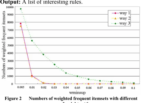
᧤i =1,2, ...,n᧥ (13) To show the applicability of these weights, we compare three different ways to set weights of items and mine weighted frequent itemsets from them using MINWAL[2]. Fig.2 shows our method is better for getting weighted frequent itemsets that have strong correlations than the two others. In way 1, the weights are simply decided by alarm levels. In way 2, the weights are decided by alarm levels and alarm types. However, the relative significances among different alarm types are not so obvious which makes for similar mining results between way 1 and way 2. As for way 3, the weights reflect information not only about the network topology, but also the degrees of relative significance of alarms. It has strong ability to distinguish the importance of alarms of different attribute- value-combinations, and could self adapt to the dynamic change of the network. Therefore, with the increase of

Z

minsup, the number of weighted frequent itemsets in way 3 drops slower than that in way 1 and way 2.

IV OUR NEW ALGORITHM—WARM

Dynamic counting technique has been explored by Brin et al. who developed the DIC algorithm [3] for itemset counting in a single database. While Apriori requires the same number of passes through the database as the size of the maximum large itemsets, dynamic counting allows candidates of various sizes to be counted at the same time in each pass. This results in the reduced number of passes through the database. What DIC does is just to create possible new candidate itemsets at every M-transaction interval while the Apriori algorithm creates new candidate itemsets only at the end of a pass through the database.

By the inspiration of DIC, we proposed an algorithm for mining weighted association rules-WARM based on

ISS(item sequence sets).

WARM algorithm has the following inputs and output. In order to describe easily, we give the following definitions and Notations:

Inputs: A database D with the transactions T, two threshold values

Z

minsup and minconf, weights of the items wi

Output: A list of interesting rules.

Figure 2 Numbers of weighted frequent itemsets with different ways of weight setting

There are two linear data structure ISS and FSS in our algorithm. The former is all the itemsets gotten from scan of the database and the latter is all the frequent itemsets generated from the algorithm. The basic idea of WARM is adding the item sequence sets of transaction t after scan it to ISS and counting the support counts of all its subsets to put those whose counts satisfy the

Z

minsup into FSS. It just likes to set the M-interval in the above DIC algorithm to 1, and can calculate all the support counts of itemsets length from 1 to |t| belong to transaction t. The procedure is described as follows.

WARM Algorithm(D,

Z

,

Z

minsup, minconf, L) {

ISS=

; FSS=

;

for all IS D //get item sequence sets of transactions in D {

add(IS,ISS);

gen_fre(IS,ISS,FSS,

Z

minsup); }

L=FSS;

Rules(Support,L); }

The sub-procedure add is used for scanning transactions in D one by one and adding them to ISS.

add(IS,ISS) {

sup_count (IS)= 1; flag=0˗

for all IS1 ISS

D the database

Z

the set of item weights

Lk set of frequent k-itemsets

Support(X) number of transactions containing itemset X

Z

minsup weighted support threshold

(5)

{

if(IS= =IS1) {

sup_count (IS1) ++; flag=1;

} }

if(flag= =0) ISS=ISS U {IS}; }

The sub-procedure gen_fre makes use of IS to select frequent itemsets in ISS, then add them to frequent item sequence sets FSS. Along with the addition of frequent itemsets, FSS will become bigger and bigger. It works as follows.

gen_fre(IS,ISS,FSS,

Z

minsup) {

for all IS* subset{IS} {

if(IS*

subset{FSS}) {

sup_count (IS*)=0 for all IS** ISS

if (IS*

IS**)

sup_count (IS*) += sup_count(IS**); if(

*

(

) (

(

*))

min sup

j

j i IS

Support IS

Z

x

t

¦

)

FSS=FSSU{IS*}; }

} }

The sub-procedure subset{IS} is to get the aggregation of all subsets of IS, it operates as follows.

Set subset(IS) {

Set<String> subsetIS=new HashSet<String>(); N=|IS|; //the length of itemsets in IS

k=0;

String[] S=new String[2N-1]; for(i=0;i<S.length;i++) S[i]= “”;

char[] c=IS.tocharArray();//construct array that makes up of all single items in IS

for(i=1;i<2N;i++) {

for(j=0;j<N;j++) if((i>>j)&1)

S[k]+=c[j]; subsetIS.add(S[k]); k++;

}

return subsetIS; }

Rules (Support,L): Find the rules from the large itemsets L, similar to [1].

WARM only needs to scan the transaction database once, and need not to generate the candidate itemsets. Therefore, we can conclude that the excellence of our algorithm over the MINWAL algorithm is not only contributed by the use of dynamic counting technique, but also the whole design

of the algorithm.

V PERFORMANCE STUDY OF EDMA

F. Generation of Synthetic Data

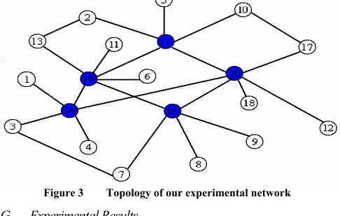
In our research, we used synthetic databases to evaluate the performance of different algorithms. Fig.3 shows the topology of our network and the alarm data is generated as following:

Alarm occurs in one of the blue nodes randomly as well as the alarm level and alarm type

Alarms of the blue nodes cause corresponding alarms in same level of all neighboring nodes and will not be transmitted further

After generating alarms, it comes to the problem of alarm's synchronization which was settled by setting time window and slip length. The attributes of the alarm that reflect the faults were picked out to form an item of an alarm transaction and the redundant alarms were got rid of by alarm compressing. The alarm's pretreatment was carried out to transform the alarm database into alarm transaction database which make ready the data for weighted alarm association rules mining.

Figure 3 Topology of our experimental network

G. Experimental Results

We have extensively studied our algorithm's performance by comparing it with the FP-tree algorithm[6] as well as MINWAL [2] and consider the superiority of it. FP-tree only scans the database twice and never generates the huge candidate itemsets, therefore reduces the temporary occupation of memory space as well as I/O cost needed for mining. However, the memory space can not be downgraded sometimes and the tree is a nonlinear structure that needs link list to storage, which increases the overhead of storing the link information.

In order to control different parameters in the experimental setup, we use synthetic databases and weights formed above in the experiment. We also use the same item weights is to keep this factor constant to confirm the efficiency of WARM with different transaction databases.

We study the effect of different values of

Z

minsup, number of transactions and items, etc., on the processing time, for algorithms weighted FP-tree, MINWAL and WARM.

(6)

and the algorithm was written in Java.

First of all, our algorithm is based on the theory and operation of item sequence sets (ISS). We generate transaction database ranging from 10K to 100K and set

Z

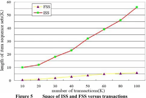
minsup=0.2, then examine how the method scales up and compare the performance of them. Fig.4 indicates that not only the whole execution time of ISS is better than Apriori, but also with increase of transactions the increasing scope of execution time of ISS is less than that of Apriori. As for weighted case, the result is a little different. The more item sequences are, the better WARM performs than MINWAL. Because when transactions grow, there are more weighted potentially frequent itemsets for the latter to generate and calculate. We can also see that WARM is more scalable than MINWAL.

Then Fig.5 describes that, with the increase of transactions the increment of FSS is mild which is much less than its theoretical value. Because our database is generated randomly, it almost has no repetition. If the repetition of database is large, it will surely cause the decline of length of ISS. Therefore, how to control the space that ISS occupy is the most needed improvement for our algorithm.

In the following, we examine how the performance varies with respect to different number of items and

Z

minsup while all other things being equal. With transaction database is 100K for all cases, a series of items range from 100 to 1K. The execution time increases with the number of items since the more the items, the larger the candidate itemsets, the global FP-tree as well as the item sequence. As all of them grow directly with the items, the execution time in the count searching would be increased, which is shown in Fig.6. From this figure, we can see the execution time of WARM is about 78% to 93% and 33% to 73% faster than MINWAL and weighted FP-tree, respectively. This denotes WARM has a steady advantage over MINWAL and weighted FP-tree in terms of different number of items and the execution time is much less than its theoretical upper limit. The slope ratio for each different size is almost similar. As the execution time is given in ln(sec), and it increases with the number of items linearly with ln scale, implying that the complexity of the algorithms is exponential in the number of items.

Figure 4 Runtime with itemsequences scale-up

Figure 5 Space of ISS and FSS versus transactions

Fig.7 displays the decreasing trend of the execution time of MINWAL when the support threshold increases. As the threshold increases, the candidate itemsets decrease. Then the execution time would decrease because of the decreasing searching time. However, weighted FP-tree and WARM are based on the conditional pattern-base (not the conditional FP-tree) and item sequence sets respectively, which are not affected by

Z

minsup. Therefore, the whole execution times of them almost keep the same among various

Z

minsup thresholds. The reduction of time about 1% to 49% and 5% to 18% are witnessed in WARM compare to MINWAL and weighted FP-tree, respectively.

The next experiment deals with relationship between the number of frequent itemsets involving some given items and these items' weight is plotted in Fig.8, when

Z

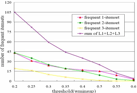
minsup=0.2 and transaction database is fixed at 10K. Here we let the respective weight of the five items (alarm1, alarm2, alarm3, alarm4 and alarm5) vary, while weights of other items held equally. Figure 8 shows the number of frequent itemsets with regard to specific item grows with the increase of the item's weight, which is as we expected. Each frequent itemset is a potential association rule, so the bigger the weight of an item is, the more the relative association rules are under predefined minconf. This also means users' subjective preference can be added into the procedure of data mining by adjusting weights.

At last, Fig.9 compares the number of weighted frequent itemsets for different

Z

minsups. We can see that the shorter the length of frequent itemsets is, the smoother the corresponding curve is. It is natural because higher requirements are asked for the candidate itemsets that include more items, which makes these itemsets are more sensitive to the change of the

Z

minsup.

VI CONCLUSION

(7)

choosing interesting rules. In addition, for each support value is normal size, similar to that in apriori algorithm, the

Z

minsup is also easy to provide or predict by the users or experts in the proposed method. Experimental results have demonstrated it outperforms the other two algorithms.

Beside, as in our communication network different data sets may spread over various geographical sites and be periodically and continually updated. Distributed mining as well as dynamic mining of association rules can be further considered.

Figure 6 Overall execution time with number of items scale-up

Figure 7 Overall execution time with

Z

minsup scale-up

Figure 8 Number of frequent itemsets versus weight

Figure 9 Number of frequent itemsets with

Z

minsup scale-up

ACKNOWLEDGMENTS

This work was supported by the Republic of China National Science Foundation under Contract No.60572091.

REFERENCES

[1] R. Agrawal and R. Srikant. Fast algorithms for mining association rules. In Proceedings of the 20th VLDB Conference, pages 487-499, 1994

[2] C.H.Cai, Ada W.C. Fu, C.H. Cheng and W.W. Kwong, Mining Association Rules with Weighted Items. Proceedings of the 1998 International Symposium on Database Engineering & Applications, Cardiff, Wales, 1998, pp. 68-77.

[3] S.Rrin, R.Motwani, J.D.UIIman, and S.Tsur. Dynamic itemset counting and implication rules for market basket data. In Proceedings of ACM SIGMOD International Conference on Management of Data, pages 255-264, AZ, 1997

[4] Saaty S, Thomas L. The Analytic Hierarchy Process [M]. New York:McGraw-Hill Company, 1980.

[5] S.L.Tung, S.L.Tang, A comparison of the Saaty's AHP and modified AHP for right and left eigenvector inconsistency. European Journal of Operational Research, ELSEVIER, 1998,123-128.

[6] J.Han, J.Pei, Y.Yin, and R.Mao. Mining frequent patterns without candidate generation: A frequent-pattern tree approach [J]. Data Mining and Knowledge Discovery, 2003.8(1):53-87

[7] Takeshi Fukuda, Yasuhiko Morimoto, Shinichi Morishita, and Takeshi Tokuyama. Mining optimized association rules for numeric attributes. Technical Report 1623-14, IBM Tokyo Research Laboratory, 1996.

[8] J. Han, M. Kamber, and J. Chiang. Mining multidimensional association rules using data cubes. Technical report, Database Systems Research Laboratory, School of Science, Simon Fraser University, 1997.

[9] J.S. Park, M-S. Chen, and P.S. Yu. An effective hash-based algorithm for mining association rules. In Proceedings of ACM SIGMOD, pages 175-186, 1995.

[10] A. Savasere, E. Omiecinski, and S. Navathe. An effcient algorithm for mining association rules in large databases. In Proceedings of the 21th International Conference on Very Large Data Bases, pages 432-444, 1995.

[11] W.J. Frawley, G. Piatetsky-Shapiro and C.J.Matheus, Knowledge discovery in databases: an overview, The AAAI Workshop on Knowledge Discovery in Databases, 1991, pp.1-27.

(8)

[13] R. Srikant and R. Agrawal, Mining quantitative association rules in large relational tables, The 1996 ACM SIGMOD International Conference on Management of Data. Montreal,Canada, June 1996,pp. 1-12.

[14] S.-F. Lu, H. Hu and F. Li, Mining weighted association rules, Intelligent Data Analysis, 5, 2001, pp. 211-225.

[15] T.-P.Hong and S.-C.Chi. Trade-off between computation time and numbers of rules for fuzzy mining from quantitative data. International Journal of Uncertainty,Fuzziness and Knowledge-based Systems 9, 2001 587-604.

[16] Mannila H., Toivonen H., and Verkamo A.I. Discovering frequent episodes in sequences. In Proceeding of the First Interntional Conference on Knowledge Discovery and Data mining, pages 210-215,Montreal, Quebec, 1995.

[17] R. Srikant and R. Agrawal. Mining sequential patterns: Generalizations and performance improvements. In Proceeding of the Fifth International Conference on Extending Database Technology, Avignon, France, 1996

Wu-Jian ( female) was born in Chengdu , China on June 20, 1981 . She received the B.S. degree in information engineering from Sichuan University in 2004. She is currently a Ph.D. candidate of Key Laboratory of Broadband Optical Fiber Transmission and Communication Networks of UESTC, specializing in Data Mining & Knowledge Discovery.

She worked in the project “The alarm correlation in communication networks based on data mining” supported by

National Science Foundation under Contract No.60572091 in 2006. Her main job included: Study the mining of the alarm weighted association rules Research the association rules from distributed data sources Learn the association rules from self-adaptation for dynamic network resource. Following are selected recent publications:

z Wu Jian and Tu Xiao dong. Analysis and Realization to

Security of Radio Frequency Identification system. In Proceedings of the 6th International Conference on ITS Telecommunications, pages 222-225, China, 2006

z Wu Jian and Li Xing ming. A Novel Algorithm for dynamic

Mining of Association Rules. In Proceedings of the 1st International Workshop on Knowledge Discovery and Data Mining, pages 94-99, Australia, 2008

z Wu Jian and Li Xing ming. An Efficient Association Rule

Mining Algorithm In Distributed Databases. In Proceedings of the 1st International Workshop on Knowledge Discovery and Data Mining, pages 108-113, Australia, 2008

An Effective Mining Algorithm for Weighted Association Rules in Communication Networks