R E S E A R C H
Open Access
JANUS: A hypothesis-driven Bayesian
approach for understanding edge formation in
attributed multigraphs
Lisette Espín-Noboa
1,2*, Florian Lemmerich
1,2, Markus Strohmaier
1,2and Philipp Singer
1,2*Correspondence: [email protected] This article extends a previous workshop publication (Espín-Noboa et al. 2016). The main novelties in this manuscript include the extension todyad-attributed networks (such as as multiplex networks), additional experimental results, and a comparison of our approach to alternative methods. 1GESIS - Leibniz Institute for the Social Sciences, Unter
Sachsenhausen 6-8, 50667 Cologne, Germany
2University of Koblenz-Landau, Universitätstraße 1, 56070 Koblenz, Germany
Abstract
Understanding edge formation represents a key question in network analysis. Various approaches have been postulated across disciplines ranging from network growth models to statistical (regression) methods. In this work, we extend this existing arsenal of methods with JANUS, a hypothesis-driven Bayesian approach that allows to intuitively compare hypotheses about edge formation in multigraphs. We model the multiplicity of edges using a simple categorical model and propose to express hypotheses as priors encoding our belief about parameters. Using Bayesian model comparison techniques, we compare the relative plausibility of hypotheses which might be motivated by previous theories about edge formation based on popularity or similarity. We demonstrate the utility of our approach on synthetic and empirical data. JANUS is relevant for researchers interested in studying mechanisms explaining edge formation in networks from both empirical and methodological perspectives.
Keywords: Edge formation, Bayesian inference, Attributed multigraphs, Multiplex,
HypTrails
Introduction
Understanding edge formation in networks is a key interest of our research commu-nity. For example, social scientists are frequently interested in studying relations between entities within social networks, e.g., how social friendship ties form between actors and explain them based on attributes such as a person’s gender, race, political affiliation or age in the network (Sampson 1968). Similarly, the complex networks community suggests a set of generative network models aiming at explaining the formation of edges focus-ing on the two core principles ofpopularityandsimilarity(Papadopoulos et al. 2012). Thus, a series of approaches to study edge formation have emerged including statistical (regression) tools (Krackhardt 1988; Snijders et al. 1995) and model-based approaches (Snijders 2011; Papadopoulos et al. 2012; Karrer and Newman 2011) specifically estab-lished in the physics and complex networks communities. Other disciplines such as the computer sciences, biomedical sciences or political sciences use these tools to answer empirical questions; e.g., co-authorship networks (Martin et al. 2013), wireless networks of biomedical sensors (Schwiebert et al. 2001), or community structures of political blogs (Adamic and Glance 2005).
Problem illustration Consider for example the network depicted in Fig. 1. Here, nodes represent authors, and (multiple) edges between them refer to co-authored scientific articles. Node attributes provide additional information on the authors, e.g., their home country and gender. In this setting, an exemplary research question could be: “Can co-authorship be better explained by a mechanism that assumes more collaborations between authors from thesame countryor by a mechanism that assumes more collabora-tions between authors with thesame gender?”. These and similar questions motivate the main objective of this work, which is to provide a Bayesian approach for understanding how edges emerge in networks based on some characteristics of the nodes or dyads.
While several methods for tackling such questions have been proposed, they come with certain limitations. For example, statistical regression methods based on QAP (Hubert and Schultz 1976) or mixed-effects models (Shah and Sinha 1989) do not scale to large-scale data and results are difficult to interpret. For network growth models (Papadopoulos et al. 2012), it is necessary to find the appropriate model for a given hypothesis about edge formation and thus, it is often not trivial to intuitively compare competing hypotheses. Consequently, we want to extend the methodological toolbox for studying edge formation in networks by proposing a first step towards a hypothesis-driven generative Bayesian framework.
Approach and methods We focus on understanding edge formation in attributed multi-graphs. We are interested in modeling and understanding the multiplicity of edges based on additional network information, i.e., given attributes for the nodes or dyads in the net-work. Our approach follows a generative storyline. First, we define the model that can characterize the edge formation at interest. We focus on the simple categorical model, from which edges are independently drawn from. Motivated by previous work on sequen-tial data (Singer et al. 2015), the core idea of our approach is to specify generative hypotheses about how edges emerge in a network. These hypotheses might be motivated by previous theories such as popularity or similarity (Papadopoulos et al. 2012)—e.g., for Fig. 1 we could hypothesize that authors are more likely to collaborate with each
other if they are from the same country. Technically, we elicit these types of hypothe-ses as beliefs in parameters of the underlying categorical model and encode and integrate them as priors into the Bayesian framework. Using Bayes factors with marginal likelihood estimations allows us to compare the relative plausibility of expressed hypotheses as they are specifically sensitive to the priors. The final output is a ranking of hypotheses based on their plausibility given the data.
Contributions The main contributions of this work are:
1. We present a first step towards a Bayesian approach for comparing generative hypotheses about edge formation in networks.
2. We provide simple categorical models based on local and global scenarios allowing the comparison of hypotheses for multigraphs.
3. We show that JANUS can be easily extended to dyad-attributed multigraphs when multiplex networks are provided.
4. We demonstrate the applicability and plausibility of JANUS based on experiments on synthetic and empirical data, as well as by comparing it to the state-of-the-art QAP.
5. We make an implementation of this approach openly available on the Web (Espín-Noboa 2016).
Structure This paper is structured as follows: First, we start with an overview of some existing research on modeling and understanding edge formation in networks in Section “Related work”. We present some background knowledge required in this work in Section “Background” to then explain step-by-step JANUS in Section “Approach”. Next, we show JANUS in action and the interpretation of results, by running four dif-ferent experiments on synthetic and empirical data in Section “Experiments”. In Section “Discussion” we suggest a fair comparison of JANUS with the Quadratic Assignment Procedure (QAP) for testing hypotheses on dyadic data. We also highlight some impor-tant caveats for further improvements. Finally, we conclude in Section “Conclusions” by summarizing the contributions of our work.
Related work
We provide a broad overview of research on modeling and understanding edge formation in networks; i.e.,edge formation modelsandhypothesis testing on networks.
models (Robins et al. 2007) (also called the p∗ class of models) represent graph dis-tributions with an exponential linear model that uses feature-structure counts such as reciprocity, k-stars and k-paths. In this line of research,p1 models(Holland and Leinhardt 1981) consider expansiveness (sender) and popularity (receiver) as fixed effects associ-ated with unique nodes in the network (Goldenberg et al. 2010) in contrast to thep2 models(Robins et al. 2007) which account for random effects and assume dyadic indepen-dence conditionally to node-level attributes. While many of these works focus on binary relationships, (Xiang et al. 2010) proposes an unsupervised model to estimate continuous-valued relationship strength for links from interaction activity and user similarity in social networks. Recently, the work in (Kleineberg et al. 2016) has shown that connections in one layer of a multiplex can be accurately predicted by utilizing the hyperbolic distances between nodes from another layer in a hidden geometric space.
Hypothesis testing on networks Previous works have implemented different tech-niques to test hypotheses about network structure. For instance, the work in (Moreno and Neville 2013) proposes an algorithm to determine whether two observed networks are significantly different. Another branch of research has specifically focused on dyadic relationships utilizing regression methods accounting for interdependencies in network data. Here, we find Multiple Regression Quadratic Assignment Procedure (MRQAP) (Krackhardt 1988) and its predecessor QAP (Hubert and Schultz 1976) which permute nodes in such a way that the network structure is kept intact; this allows to test for signif-icance of effects.Mixed-effects models(Shah and Sinha 1989) add random effects to the models allowing for variation to mitigate non-independence between responses (edges) from the same subject (nodes) (Winter 2013). Based on thequasi essential graphthe work in (Nguyen 2012) proposes to compare two graphs (i.e., Bayesian networks) by testing and comparing multiple hypotheses on their edges. Recently,generalized hypergeometric ensembles(Casiraghi et al. 2016) have been proposed as a framework for model selec-tion and statistical hypothesis testing of finite, directed and weighted networks that allow to encode several topological patterns such as block models where homophily plays an important role in linkage decision. In contrast to our work, neither of these approaches is based on Bayesian hypothesis testing, which avoids some fundamental issues of classic frequentist statistics.
Background
In this paper, we focus on bothnode-attributed anddyad-attributed multigraphs with unweighted edges without own identity. That means, each pair of nodes or dyad can be connected by multiple indistinguishable edges, and there are features for the individual nodes or dyads available.
Node-attributed multigraphs We formally define this as: Let G = (V,E,F) be an unweighted attributed multigraph with V = (v1,. . .,vn) being a list of nodes, E =
{(vi,vj)} ∈ V ×V a multiset of either directed or undirected edges, and a set of
fea-ture vectorsF = (f1,. . .,fn). Each feature vector fi = (fi[ 1] , ...,fi[c])T maps a node
vito c(numeric or categorical) attribute values. The graph structure is captured by an
number of edges between nodesviandvj). By definition, the total number of multiedges
isl= |E| =ijmij.
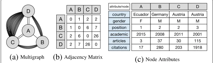
Figure 1a shows an example unweighted attributed multigraph: nodes represent authors, and undirected edges represent co-authorship in scientific articles. The adja-cency matrix of this graph—counting for multiplicity of edges—is shown in Fig. 1b. Feature vectors (node attributes) are described in Fig. 1c. Thus, for this particular case, we account forn=4 nodes,l=44 multiedges, andc=6 attributes.
Dyad-attributed networks As an alternative to attributed nodes, we also consider multigraphs, in which each dyad (pair of nodes) is associated with a set of featuresFˆ = (fˆ11,. . .,fˆnn). Each feature vectorfˆij =(fˆij[ 1] , ...,fˆij[c])T maps the pair of node (vi,vj) to
c(numeric or categorical) attribute values. The values of each feature can be represented in a separaten×nmatrix. As an important special case of dyad-attributed networks, we studymultiplex networks. In these networks, all dyad features are integer-valued. Thus, each feature can be interpreted as (or can be derived from) a separate multigraph over the same set of nodes. In our setting, the main idea is then to try and explain the occurrence of a multiset of edgesEin one multigraphGwith nodesV by using other multigraphsGˆ on the same node set.
Bayesian hypothesis testing Our approach compares hypotheses on edge formation based on techniques from Bayesian hypothesis testing (Kruschke 2014; Singer et al. 2015). The elementary Bayes’ theorem states for parametersθ, given dataDand a hypothesisH that:
posterior
P(θ|D,H)=
likelihood
P(D|θ,H)
prior
P(θ|H) P(D|H)
marginal likelihood
(1)
As observed data D, we use the adjacency matrix M, which encodes edge counts.θ refers to the model parameters, which in our scenario correspond to the probabilities of individual edges.H denotes a hypothesis under investigation. Thelikelihooddescribes, how likely we observe data D given parameters θ and a hypothesis H. The prior is the distribution of parameters we believe in before seeing the data; in other words, the prior encodes our hypothesis H. Theposterior represents an adjusted distribution of parameters after we observe D. Finally, the marginal likelihood (also called evidence) represents the probability of the dataDgiven a hypothesisH.
Approach
In this section, we describe the main steps towards a hypothesis-driven Bayesian approach for understanding edge formation in unweighted attributed multigraphs. To that end, we propose intuitive models for edge formation (Section “Generative edge for mation models”), a flexible toolbox to formally specify belief in the model parameters (Section “Constructing belief matrices”), a way of computing proper (Dirichlet) priors from these beliefs (Section “Eliciting a Dirichlet prior”), computation of the marginal like-lihood in this scenario (Section “Computation of the marginal likelike-lihood”), and guidelines on how to interpret the results (Section “Application of the method and interpretation of results”). We subsequently discuss these issues one-by-one.
Generative edge formation models
We propose two variations of our approach, which employ two different types of generative edge formation models in multigraphs.
Global model First, we utilize a simpleglobal model, in which a fixed number of graph edges are randomly and independently drawn from the set of all potential edges in the graphG by sampling with replacement. Each edge (vi,vj) is sampled from a
cat-egorical distribution with parameters θij, 1 ≤ i ≤ n, 1 ≤ j ≤ n,∀ij : ijθij = 1:
(vi,vj) ∼ Categorical(θij). This means that each edge is associated with one probability
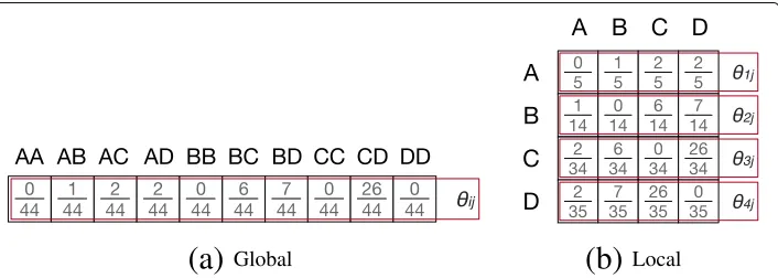
θij of being drawn next. Figure 2a shows the maximum likelihood global model for the network shown in Fig. 1. Since this is an undirected graph, inverse edges can be ignored resulting inn(n+1)/2 potential edges/parameters.
Local models As an alternative, we can also focus on alocal level. Here, we model to which other node a specific nodevwill connectgiven that any new edge starting from vis formed. We implement this by using a set of n separate models for the outgoing edges of the ego-networks (i.e., the 1-hop neighborhood) of each of thennodes. The ego-network model for nodevi is built by drawing randomly and independently a
num-ber of nodesvjby sampling with replacement and adding an edge fromvito this node.
Each nodevj is sampled from a categorical distribution with parameters θij, 1 ≤ i ≤
n, 1 ≤ j ≤ n,∀i : jθij = 1:vj ∼ Categorical(θij). The parametersθij can be
writ-ten as a matrix; the value in cell(i,j)specifies the probability that a new formed edge
with source nodevi will have the destination nodevj. Thus, all values within one row
always sum up to one. Local models can be applied for undirected and directed graphs (cf. also in Section “Discussion”). In the directed case, we model only the outgoing edges of the ego-network. Figure 2b depicts the maximum likelihood local models for our introductory example.
Hypothesis elicitation
The main idea of our approach is to encode our beliefs in edge formation as Bayesian priors over the model parameters. As a common choice, we employ Dirichlet distribu-tions as theconjugate priorsof the categorical distribution. Thus, we assume that the model parametersθ are drawn from a Dirichlet distribution with hyperparameters α: θ ∼Dir(α). Similar to the model parameters themselves, the Dirichlet prior (or multiple priors for the local models) can be specified in a matrix. We will choose the parameters α in such a way that they reflect a specific belief about edge formation. For that pur-pose, we first specify matrices that formalize these beliefs, then we compute the Dirichlet parametersαfrom these beliefs.
Constructing belief matrices
We specify hypotheses about edge formation asbelief matrices B= bij. These aren×n
matrices, in which each cellbij∈IR represents a belief of having an edge from nodevito
nodevj. To express a belief that an edge occurs more often (compared to other edges) we
setbijto a higher value.
Node-attributed multigraphs In general, users have a large freedom to generate belief matrices. However, typical construction principles are to assume that nodes with spe-cific attributes are more popular and thus edges connecting these attributes receive higher multiplicity, or to assume that nodes that aresimilarwith respect to one or more attributes are more likely to form an edge, cf. (Papadopoulos et al. 2012). Ideally, the elicitation of belief matrices is based on existing theories.
For example, based on the information shown in Fig. 1, one could “believe” that two authors collaboratemore frequentlytogether if: (1) they both are from the same country, (2) they share the same gender, (3) they have high positions, or (4) they are popular in terms of number of articles and citations. We capture each of these beliefs in one matrix. One implementation of the matrices for our example beliefs could be:
• B1(same country):bij:=0.9iffi[country]=fj[country]and 0.1 otherwise
• B2(same gender):bij:=0.9iffi[gender]=fj[gender]and 0.1 otherwise
• B3(hierarchy):bij:=fi[position]·fj[position]
• B4(popularity):bij:=fi[articles]+fj[articles]+fi[citations]+fj[citations]
Figure 3a shows the matrix representation of belief B1, and Fig. 3b its respective
row-wise normalization for the local model case. While belief matrices are identically structured for local and global models, the ratio between parameters in different rows is crucial for the global model, but irrelevant for local ones.
Fig. 3Prior belief: This figure illustrates the three main phases of prior elicitation. That is,aa matrix representation of beliefB1, where authors are more likely to collaborate with each other if they are from the same country.bB1normalized row-wise using the local model interpretation.cPrior elicitation forκ=4; i.e.,
αij= bZij×κ+1
co-authorshipnetwork—where every node represents an author with no additional infor-mation or attribute—could be explained by acitationnetwork under the hypothesis that if two authors frequently cite each other, they are more likely to also co-author together. Thus, the adjacency (feature) matrices(F)ˆ of secondary multigraphs can be directly used as belief matricesB= (bij). However, we can express additional beliefs by transforming
the matrices. As an example, we can formalize the belief that the presence of a feature tends to inhibit the formation of edges in the data by settingbij:= −sigm(fij), wheresigm
is a sigmoid function such as the logistic function.
Eliciting a Dirichlet prior.
In order to obtain the hyperparameters α of a prior Dirichlet distribution, we utilize the pseudo-count interpretation of the parametersαij of the Dirichlet distribution, i.e.,
a value of αij can be interpreted as αij − 1 previous observations of the respective event forαij ≥ 1. We distribute pseudo-counts proportionally to a belief matrix. Con-sequently, the hyperparameters can be expressed as: αij = bZij × κ + 1, where κ is
the concentration parameter of the prior. The normalization constantZ is computed as the sum of all entries of the belief matrix in the global model, and as the respec-tive row sum in the local case. We suggest to set κ = n× k for the local models, κ=n2×kfor the directed global case,κ= n(n+1)
2 ×kfor the undirected global case, and
k= {0, 1, ..., 10}. A high value ofκexpresses a strong belief in the prior parameters. A sim-ilar alternative method to obtain Dirichlet priors is thetrial roulette method(Singer et al. 2015). For the global model variation, allαvalues are parameters for the same Dirichlet distribution, whereas in the local model variation, each row parametrizes a separate Dirichlet distribution. Figure 3 (c) shows the prior elicitation of beliefB1 forkappa= 4 using the local model.
Computation of the marginal likelihood
For comparing the relative plausibility of hypotheses, we use the marginal likelihood. This is the aggregated likelihood over all possible values of the parametersθ weighted by the Dirichlet prior. For our set of local models we can calculate them as:
P(D|H)=
n
i=1
nj=1αij
nj=1αij+mij n
j=1
(αij+mij)
(αij)
Recall,αij encodes our prior belief connecting nodesvi andvj inG, andmij are the
actual edge counts. Since we evaluate only a single model in the global case, the product over rowsiof the adjacency matrix can be removed, and we obtain:
P(D|H)=
ni=1nj=1αij
ni=1nj=1αij+mij n
i=1 n
j=1
αij+mij
(αij)
(3)
Section “Computation of the marginal likelihood” holds for directed networks. In the undirected case, indicesjgo fromitonaccounting for only half of the matrix including the diagonal to avoid inconsistencies. For a detailed derivation of the marginal likelihood given a Dirichlet-Categorical model see (Tu 2014; Singer et al. 2014). For both models we focus on the log-marginal likelihoods in practice to avoid underflows.
Bayes factor Formally, we compare the relative plausibility of hypotheses by using so-calledBayes factors(Kass and Raftery 1995), which simply are the ratios of the marginal likelihoods for two hypothesesH1andH2. If it is positive, the first hypothesis is judged as
more plausible. The strength of the Bayes factor can be checked in an interpretation table provided by Kass and Raftery (1995).
Application of the method and interpretation of results
We now showcase an example application of our approach featuring the network shown in Fig. 1, and demonstrate how results can be interpreted.
Hypotheses We compare four hypotheses (represented as belief matrices) B1,B2,B3,
andB4 elaborated in Section “Hypothesis elicitation”. Additionally, we use theuniform
hypothesis as abaseline. It assumes that all edges are equally likely, i.e.,bij = 1 for all
i,j. Hypotheses that are not more plausible than the uniform cannot be assumed to cap-ture relevant underlying mechanisms of edge formation. We also use thedatahypothesis as an upper bound for comparison, which employs the observed adjacency matrix as belief:bij=mij.
Calculation and visualization For each hypothesis H and everyκ, we can elicit the Dirichlet priors (cf. Section “Hypothesis elicitation”), determine the aggregated marginal likelihood (cf. Section “Computation of the marginal likelihood)”, and compare the plausi-bility of hypotheses compared to the uniform hypothesis at the sameκby calculating the logarithm of the Bayes factor aslog(P(D|H))−log(P(D|Huniform)). We suggest two ways of
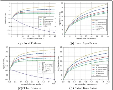
visualizing the results, i.e., plotting the marginal likelihood values, and showing the Bayes factors on the y-axis as shown in Fig. 4a and 4b respectively for the local model. In both cases, the x-axis refers to the concentration parameterκ. While the visualization show-ing directly the marginal likelihoods carries more information, visualizshow-ing Bayes factors makes it easier to spot smaller differences between the hypotheses.
Fig. 4Ranking of hypotheses for the introductory example.a,bRepresent results using the local model and
c,dresults of the global model. Rankings can be visualized usinga,cthe marginal likelihood or evidence (y-axis), orb,dusing Bayes factors (y-axis) by setting the uniform hypothesis as a baseline to compare with; higher values refer to higher plausibility. The x-axis depicts the concentration parameterκ. For this example, from an individual perspective (local model) authors from the multigraph shown in Fig. 1 appear to prefer to collaborate more often with researchers of the same country rather than due to popularity (i.e., number of articles and citations). In this particular case, the same holds for the global model. Note that all hypotheses outperform the uniform, meaning that they all are reasonable explanations of edge formation for the given graph
interpret this as further evidence for the plausibility of expressed hypothesis as this means that the more we believe in it, the higher the Bayesian approach judges its plausibility. As a result for our example, we see that the hypothesis believing that two authors are more likely to collaborate if they are from the same country is the most plausible one (after the data hypothesis). In this example, all hypotheses appear to be more plausible than the baseline in both local and global models, but this is not necessarily the case in all applications.
Experiments
We demonstrate the utility of our approach on both synthetic and empirical networks.
Synthetic node-attributed multigraph
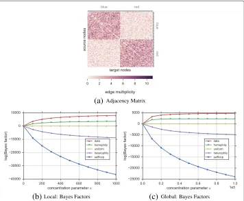
Network The network contains 100 nodes where each node is assigned one of two colors with uniform probability. For each node, we then randomly drew 200 undirected edges where each edge connects randomly with probabilityp = 0.8 to a different node of the same color, and withp=0.2 to a node of the opposite color. The adjacency matrix of this graph is visualized in Fig. 5a.
Hypotheses In addition to the uniform baseline hypothesis, we construct two intu-itive hypotheses based on the node color that express belief in possible edge formation mechanics. First, the homophilyhypothesis assumes that nodes of the same color are more likely to have more edges between them. Therefore, we arbitrary set belief values bij to 80 when nodesviandvjare of the same color, and 20 otherwise. Second, the
het-erophilyhypothesis expresses the opposite behavior; i.e.,bij =80 if the color of nodesvi
andvjare different, and 20 otherwise. An additionalselfloophypothesis only believes in
self-connections (i.e., diagonal of adjacency matrix).
Results Figure 5b and 5c show the ranking of hypotheses based on their Bayes factors compared to the uniform hypothesis for the local and global models respectively. Clearly,
in both models the homophily hypothesis is judged as the most plausible. This is expected and corroborates the fact that network connections are biased towards nodes of the same color. The heterophily and selfloop hypotheses show negative Bayes factors; thus, they are not good hypotheses about edge formation in this network. Due to the fact that the multi-graph lacks of selfloops, the selfloop hypothesis decreases very quickly with increasing strength of beliefκ.
Synthetic multiplex network
In this experiment, we control the underlying mechanisms of how edges in a dyad-attributed multigraph emerge using multiple multigraphs that share the same nodes with different link structure (i.e., multiplex) and thus, expect these also to be good hypotheses for JANUS.
Network The network is an undirectedconfiguration modelgraph (Newman 2003) with parametersn = 100 (i.e., number of nodes) and degree sequence−→k = ki drawn from
a power law distribution of lengthnand exponent 2.0, wherekiis the degree of nodevi.
The adjacency matrix of this graph is visualized in Fig. 6a.
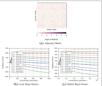
Hypotheses Besides the uniform hypothesis, we include ten more hypotheses derived from the original adjacency matrix of the configuration model graph where only certain percentageof edges get shuffled. The bigger thethe less plausible the hypothesis since more shuffles can modify drastically the original network.
Results Figure 6b and 6c show the ranking of hypotheses based on their Bayes fac-tors compared to the uniform hypothesis for the local and global model respectively. In general, hypotheses are ranked as expected, from small to big values of. For instance, theepsilon10phypothesis explains best theconfiguration model graph—represented in Fig. 6a—since it only shuffles 10% of all edges (i.e., 10 edges). On the other hand the epsilon100phypothesis shows the worst performance (i.e., Bayes factor is negative and far from the data curve) since it shuffles all edges, therefore it is more likely to be different than the original network.
Empirical node-attributed multigraph
Here, we focus on a real-world contact network based on wearable sensors.
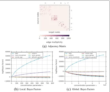
Network We study a network capturing interactions of 5 households in rural Kenya between April 24 and May 12, 2012 (Sociopatterns; Kiti et al. 2016). The undirected unweighted multigraph contains 75 nodes (persons) and 32, 643 multiedges (contacts) which we aim to explain. For each node, we know information such as gender and age (encoded into 5 age intervals). Interactions exist within and across households. Figure 7a shows the adjacency matrix (i.e., number of contacts between two people) of the network. Household membership of nodes (rows/columns) is shown accordingly.
Hypotheses We investigate edge formation by comparing—next to the uniform base-line hypothesis—four hypotheses based on node attributes as prior beliefs. (i) Thesimilar agehypothesis expresses the belief that people of similar age are more likely to inter-act with each other. Entriesbijof the belief matrixBare set to the inverse age distance
between members: 1+abs(f 1
i[age]−fj[age]). (ii) Thesame household hypothesis believes that people are more likely to interact with people from the same household. We arbitrarily setbijto 80 if personvi and personvjbelong to the same household, and 20 otherwise.
(iii) With thesame genderhypothesis we hypothesize that the number of same-gender interactions is higher than the different-gender interactions. Therefore, every entrybijof
Bis set to 80 if personsviandvjare of the same gender, and 20 otherwise. Finally, (iv)
thedifferent genderhypothesis believes that it is more likely to find different-gender than same-gender interactions;bijis set to 80 if personvihas the opposite gender of personvj,
and 20 otherwise.
Fig. 7Ranking of hypotheses for Kenya contact network.aShows the adjacency matrix of the network with node ordering according to household membership. Darker cells indicate more contacts.b,cDisplay the ranking of hypotheses based on Bayes factors, using the uniform hypothesis as baseline for the local and global model respectively. Using the local modelbthesame householdhypothesis ranks highest followed by thesimilar agehypothesis which also provides positive Bayes Factors. On the other hand, thesameand different genderhypotheses are less plausible than the baseline (uniform edge formation) in both the local and global case. In the global casecall hypotheses are bad representations of edge formation in the Kenya contact network. This is due to the fact that interactions are very sparse, even within households. Results are consistent for allκ
this network. This gives us a better understanding of potential mechanisms producing underlying edges. People prefer to contact people from the same household and similar age, but not based on gender preferences. Additional experiments could further refine these hypotheses (e.g., combining them). In the general case of the global model in Fig. 7c all hypotheses are bad explanations of the Kenya network. However, thesame-household hypothesis tends to go upfront the uniform for higher values ofκ, but still far form the data curve. This happens due to the fact that the interaction network is very sparse (even within same households), thus, any hypothesis with a dense belief matrix will likely fall below or very close to the uniform.
Empirical multiplex network
This empirical dataset consists of four real-world social networks, each of them extracted from Twitter interactions of a particular set of users.
of a new particle with the features of the elusive Higgs boson on the 4th of July 2012 (De Domenico et al. 2013). Specifically, we are interested on characterizing edge for-mation in thereply network, a directed unweighted multigraph which encodes the replies that a personvisent to a personvjduring the event. This graph contains 38, 918 nodes
and 36, 902 multiedges (if all edges from the same dyad are merged it accounts for 32, 523 weighted edges).
Hypotheses We aim to characterize the reply network by incorporating other networks—sharing the same nodes but different network structure—as prior beliefs. In this way we can learn whether the interactions present in the reply network can be better explained by a retweet or mentioning or following (social) network. Theretweet hypoth-esis expresses our belief that the number of replies is proportional to the number of retweets. Hence, beliefsbijare set to the number of times userviretweeted a post from
user vj. Similar as before, themention hypothesis states that the number of replies is
proportional to the number of mentions. Therefore, every entrybij is set to the
num-ber of times uservimentioned uservjduring the event. Thesocialhypothesis captures
our belief that users are more likely to reply to their friends (in the Twitter jargon: fol-lowees or people they follow) than to the rest of users. Thus, we setbij to 1 if uservi
follows uservjand 0 otherwise. Finally, we combine all the above networks to construct
theretweet-mention-socialhypothesis which captures all previous hypotheses at once. In other words, it reflects our belief that users are more likely to reply to their friends and (at the same time) the number of replies is proportional to the number of retweets and men-tions. Therefore the adjacency matrix for this hypothesis is simply the sum of the three networks described above.
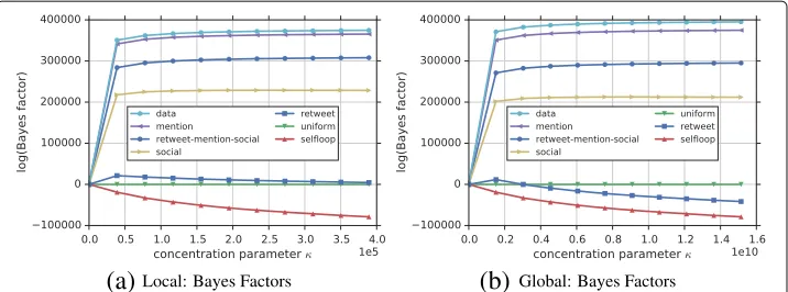
Results The results shown in Fig. 8 suggest that the mentionhypothesis explains the reply network very well, since it has been ranked first and it is very close to the data curve, in both Fig. 8a and 8b for the local and global models, respectively. The retweet-mention-socialhypothesis also indicates plausibility since it outperforms the uniform (i.e., positive Bayes factors). However, if we look at each hypothesis individually, we can see that the combined hypothesis is dominated mainly by thementionhypothesis. Thesocial hypoth-esis is also a good explanation of the number of replies since it outperforms the uniform hypothesis.RetweetsandSelf-loopson the other hand show negative Bayes factors, sug-gesting that they are not good explanations of edge formation in the reply network. Note that the retweet curve in the local model has a very strong tendency to go below the uniform for higher numbers ofκ. These results suggest us that the number of replies is proportional to the number of mentions and that usually people prefer to reply other users within their social network (i.e., followees).
Discussion
Next, we discuss some aspects and open questions related to the proposed approach.
Fig. 8Ranking of hypotheses for Reply Higgs Network.a,bRanking of hypotheses based on Bayes factors when compared to the uniform hypothesis using multiplexes for the local and global models respectively. In both cases, thementionhypothesis explains best the reply network, since it is ranked first and very close to the data curve. This might be due to the fact that replies inherit a user mention from whom a tweet was originally posted. We can see that the combinedretweet-mention-socialhypothesis is the second best explanation of the reply network. This is mainly due to the mention hypothesis which performs extremely better than the other two (social and retweet). Thesocialhypothesis can also be considered a good explanation since it outperforms the uniform. Theretweethypothesis tends to perform worse than the uniform in both cases for increasing number ofκ. Similarly, theselfloophypothesis drops down below the uniform since there are only very few selfloops in thereplynetwork data
of beliefs as expressed by the belief matrices is to compute a Pearson correlation coeffi-cient between the entries in the belief matrix and the respective entries in the adjacency matrix of the network. To circumvent the difficulties of correlating matrices, they can be flattened to vectors that are then passed to the correlation calculation. Then, hypotheses can be ranked according to their resulting correlation against the data. However, by flat-tening the matrices, we disregard the direct relationship between nodes in the matrix and introduce inherent dependencies to the individual data points of the vectors used for Pear-son calculation. To tackle this issue, one can utilize the Quadratic Assignment Procedure (QAP) as mentioned in Section “Related work”. QAP is a widely used technique for testing hypotheses on dyadic data (e.g., social networks). It extends the simple Pearson correla-tion calculacorrela-tion step by a significance test accounting for the underlying link structure in the given network using shuffling techniques. For a comparison with our approach, we executed QAP for all datasets and hypotheses presented in Section “Experiments” using
theqaptestfunction included in thestatnet(Handcock et al. 2008; Handcock et al.
2016) package inR(R Core Team 2016).
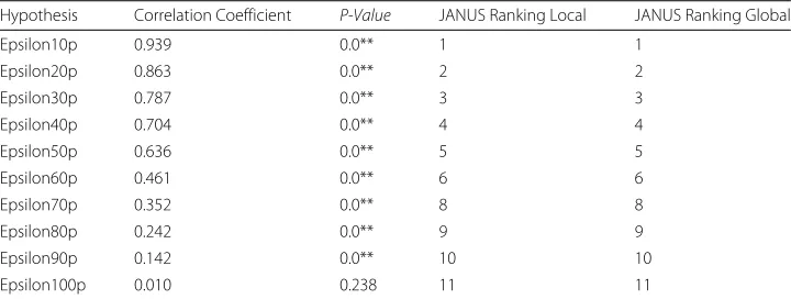
Overall, we find in all experiments strong similarities between the ranking provided by the correlation coefficients of QAP and our rankings according to JANUS. Exemplary, Table 1 shows the correlation coefficients and p-values obtained with QAP for each hypothesis tested on the synthetic multiplex described in Section “Syntheticmultiplex network” as well as the ranking of hypotheses obtained from JANUS for the local and global model (leaving the uniform hypothesis out). However, in other datasets minor differences in the ordering of the hypotheses could be observed between the two approaches.
Table 1QAP on synthetic dyad-attributed network (multiplex): List of correlation coefficients for each hypothesis tested. Last two columns show ranking of hypotheses according to JANUS for the local and global models. By omitting the uniform hypothesis in JANUS (rank 7) we can see that the ranking of hypotheses by correlation aligns with the rankings given by JANUS for the multiplex given in Section “Synthetic multiplex network”
Hypothesis Correlation Coefficient P-Value JANUS Ranking Local JANUS Ranking Global
Epsilon10p 0.939 0.0** 1 1
Epsilon20p 0.863 0.0** 2 2
Epsilon30p 0.787 0.0** 3 3
Epsilon40p 0.704 0.0** 4 4
Epsilon50p 0.636 0.0** 5 5
Epsilon60p 0.461 0.0** 6 6
Epsilon70p 0.352 0.0** 8 8
Epsilon80p 0.242 0.0** 9 9
Epsilon90p 0.142 0.0** 10 10
Epsilon100p 0.010 0.238 11 11
Statistically highly significantp-values (p<0.001) are marked by (**)
more fine-grained and advanced insights into the relative plausibility of hypotheses. Con-trary, simple correlation takes the hypothesis as it is and calculates a single correlation coefficient that does not allow for tolerances.
Second, by building upon Bayesian statistics, the significance (or decisiveness) of results in our approach is determined by Bayes factors, a Bayesian alternative to traditional p-value testing. Instead of just measuring evidenceagainst one null hypothesis, Bayes Factors allow to directly gather evidencein favorof a hypothesis compared to another hypothesis, which is arguably more suitable for ranking.
Third, QAP and MRQAP, and subsequently correlation and regression, are subject to multiple assumptions which our generative Bayesian approach circumvents. Currently, we employ QAP with simplistic linear Pearson correlation coefficients. However, one could argue that count data (multiplicity of edges) warrants advanced generalized linear models such as Poisson regression or Negative Binomial regression models.
Furthermore, our approach intuitively allows to model not only the overall network, but also the ego-networks of the individual nodes using the local models presented above. Finally, correlation coefficients cannot be applied for all hypotheses. Specifically, it is not possible to compute it for the uniform hypothesis since in this case all values in the flat-ten vector are identical. However, our method currently does not sufficiently account for dependencies within the network as it is done by specialized QAP significance tests. Exploring this issue and extending our Bayesian approach into this direction will be a key subject of future work.
Local vs global model In this paper, we presented two variations of our approach, i.e., a local and a global model. Although both model substantially different generation processes (an entire network vs. a set of ego-networks), our experiments have shown that hypotheses in the global scenario are ranked mostly the same as the ones using the local model. This is also to be expected to some degree since the constructed hypotheses did not explicitly expressed a belief that outgoing links are more likely for some nodes.
Inconsistency of local model For directed networks, the local ego-network models can assemble a full graph model by defining a probability distribution of edges for every source node. For undirected networks, this is not directly possible as e.g., the ego-network model forvAgenerated an edge fromvAtovB, but the ego-network model for nodevBdid not
generate any edge tovA. Note that this does not affect our comparison of hypotheses as
we characterize the network.
Single Edges As mentioned in Section “Background”, JANUS focuses on multigraphs, meaning that edges might appear more than once. This is because we assume that a given nodevi, with some probabilitypij, will be connectedmultipletimes to any other nodevj
in the local models. The same applies to the global model where we assume that a given edge (vi,vj)will appearmultiple times within the graph with some probabilitypij. For
the specific case of single edges (i.e., unweighted graphs), wheremij ∈ {0, 1}, one might
consider other probabilistic models to represent such graphs.
Sparse data-connections Most real networks exhibit small world properties such as high clustering coefficient and fat-tailed degree distributions meaning that the adjacency matrices are sparse. While comparison still relatively judges the plausibility, all hypothe-ses perform weak compared to the data curve as shown in Fig. 7. As an alternative, one might want to limit our beliefs to only those edges that exist in the network, i.e., we would then only build hypotheses on how edge multiplicity varies between edges.
Other limitations and future work The main intent of this work is the introduction of a hypothesis-driven Bayesian approach for understanding edge formation in networks. To that end, we showcased this approach on simple categorical models that warrant extensions, e.g., by incorporating appropriate models for other types of networks such as weighted or temporal networks. We can further investigate how to build good hypothe-ses by leveraging all node attributes, and infer subnetworks that fit best each of the given hypotheses. In the future, we also plan an extensive comparison to other methods such as mixed-effects models andp∗models. Ultimately, our models also warrant extensions to adhere to the degree sequence in the network, e.g., in the direction of multivariate hypergeometric distributions as recently proposed in (Casiraghi et al. 2016).
Conclusions
on synthetic and empirical data. For illustration purposes our examples are based on small networks. We tested our approach with larger networks obtaining identical results. We briefly compare JANUS with existing methods and discuss some advantages and disad-vantages over the state-of-the-art QAP. In future, our concepts can be extended to further models such as models adhering to fixed degree sequences. We hope that our work contributes new ideas to the research line of understanding edge formation in complex networks.
Acknowledgements
This work was partially funded by DFG German Science Fund research projects “KonSKOE” and “PoSTs II”.
Availability of data and materials
The data sets supporting the results of this article are openly available on the Web. The source code and data for toy-example and synthetic experiments can be found on GitHub: https://github.com/lisette-espin/JANUS. The rest of data sets can be found in their respective project websites: Kenya contact network in http://www.sociopatterns.org/ datasets/kenyan-households-contact-network/, and the Higgs Twitter dataset in https://snap.stanford.edu/data/higgs-twitter.html.
Authors’ contributions
LE, PS and FL conceived and designed the experiments. LE, performed the experiments. LE, PS and FL analyzed the data. LE, PS and FL contributed reagents/materials/analysis tools: LE PS FL. LE, PS, FL and MS wrote the paper. All authors read and approved the final manuscript.
Competing interests
The authors declare that they have no competing interests.
Publisher’s Note
Springer Nature remains neutral with regard to jurisdictional claims in published maps and institutional affiliations.
Received: 18 March 2017 Accepted: 25 May 2017
References
Adamic LA, Glance N (2005) The political blogosphere and the 2004 us election: divided they blog. In: Proceedings of the 3rd Int. Workshop on Link Discovery. ACM, New York. pp 36–43. doi:10.1145/1134271.1134277
Becker M, Mewes H, Hotho A, Dimitrov D, Lemmerich F, Strohmaier M (2016) Sparktrails: A mapreduce implementation of hyptrails for comparing hypotheses about human trails. In: Proceedings of the 25th International Conference Companion on World Wide Web. International World Wide Web Conferences Steering Committee, Republic and Canton of Geneva. pp 17–18. doi:10.1145/2872518.2889380
Casiraghi G, Nanumyan V, Scholtes I, Schweitzer F (2016) Generalized hypergeometric ensembles: Statistical hypothesis testing in complex networks. CoRR abs/1607.02441. arXiv:1607.02441
De Domenico M, Lima A, Mougel P, Musolesi M (2013) The anatomy of a scientific rumor. Sci Rep 3:2980 EP Espín-Noboa L (2016) JANUS. https://github.com/lisette-espin/JANUS. Accessed 10 Mar 2017
Espín-Noboa L, Lemmerich F, Strohmaier M, Singer P (2017) A hypotheses-driven bayesian approach for understanding edge formation in attributed multigraphs. In: International Workshop on Complex Networks and Their Applications. Springer, Cham. pp 3–16. doi:10.1007/978-3-319-50901-3_1
Goldenberg A, Zheng AX, Fienberg SE, Airoldi EM (2010) A survey of statistical network models. Found Trends® Mach Learn 2(2):129–233
Handcock MS, Hunter DR, Butts CT, Goodreau SM, Morris M (2008) statnet: Software tools for the representation, visualization, analysis and simulation of network data. J Stat Softw 24(1):1–11
Handcock MS, Hunter DR, Butts CT, Goodreau SM, Krivitsky PN, Bender-deMoll S, Morris M (2016) Statnet: Software Tools for the Statistical Analysis of Network Data. The Statnet Project (http://www.statnet.org). The Statnet Project (http:// www.statnet.org). R package version 2016.4. CRAN.R-project.org/package=statnet. Accessed 31 May 2017 Holland PW, Leinhardt S (1981) An exponential family of probability distributions for directed graphs. J Am Stat Assoc
76(373):33–50
Hubert L, Schultz J (1976) Quadratic assignment as a general data analysis strategy. Br J Math Stat Psychol 29(2):190–241 Karrer B, Newman ME (2011) Stochastic blockmodels and community structure in networks. Phys Rev E 83(1):016107 Kass RE, Raftery AE (1995) Bayes factors. J Am Stat Assoc 90(430):773–795
Kim M, Leskovec J (2011) Modeling social networks with node attributes using the multiplicative attribute graph model. In: UAI 2011, Barcelona, Spain, July 14–17, 2011. pp 400–409
Kiti MC, Tizzoni M, Kinyanjui TM, Koech DC, Munywoki PK, Meriac M, Cappa L, Panisson A, Barrat A, Cattuto C, et al (2016) Quantifying social contacts in a household setting of rural kenya using wearable proximity sensors. EPJ Data Sci 5(1):1 Kleineberg KK, Boguñ (á M, Serrano MÁ, Papadopoulos F (2016) Hidden geometric correlations in real multiplex
networks. Nature Physics 12:1076–1081. http://dx.doi.org/10.1038/nphys3812
Kruschke J (2014) Doing Bayesian Data Analysis: A Tutorial with R, JAGS, and Stan. Academic Press, Boston Martin T, Ball B, Karrer B, Newman M (2013) Coauthorship and citation patterns in the physical review. Phys Rev E
88(1):012814
Moreno S, Neville J (2013) Network hypothesis testing using mixed kronecker product graph models. In: Data Mining (ICDM), Dallas, Texas. IEEE. pp 1163–1168
Newman ME (2003) The structure and function of complex networks. SIAM Rev 45(2):167–256
Nguyen HT (2012) Multiple hypothesis testing on edges of graph: a case study of bayesian networks. https://hal.archives-ouvertes.fr/hal-00657166
Papadopoulos F, Kitsak M, Serrano MÁ, Boguná M, Krioukov D (2012) Popularity versus similarity in growing networks. Nature 489(7417):537–540
Pfeiffer III JJ, Moreno S, La Fond T, Neville J, Gallagher B (2014) Attributed graph models: Modeling network structure with correlated attributes. In: WWW. ACM, New York. pp 831–842
R Core Team (2016) R: A Language and Environment for Statistical Computing. R Foundation for Statistical Computing, Vienna, Austria. R Foundation for Statistical Computing. https://www.R-project.org/. Accessed 31 May 2017 Robins G, Pattison P, Kalish Y, Lusher D (2007) An introduction to exponential random graph (p*) models for social
networks. Soc Netw 29(2):173–191
Sampson SF (1968) A Novitiate in a Period of Change: An Experimental and Case Study of Social Relationships. Cornell University, Ithaca
Schwiebert L, Gupta SK, Weinmann J (2001) Research challenges in wireless networks of biomedical sensors. In: Proceedings of the 7th Annual International Conference on Mobile Computing and Networking. ACM, New York. pp 151–165
Shah KR, Sinha BK (1989) Mixed Effects Models. In: Theory of Optimal Designs. Springer, New York. pp 85–96 Singer P, Helic D, Taraghi B, Strohmaier M (2014) Detecting memory and structure in human navigation patterns using
markov chain models of varying order. PloS One 9(7):102070
Singer P, Helic D, Hotho A, Strohmaier M (2015) Hyptrails: A bayesian approach for comparing hypotheses about human trails on the web. WWW, International World Wide Web Conferences Steering Committee, Republic and Canton of Geneva. pp 1003–1013. doi:10.1145/2736277.2741080
SNAP Higgs Twitter datasets. https://snap.stanford.edu/data/higgs-twitter.html. Accessed 15 Aug 2016
Snijders T, Spreen M, Zwaagstra R (1995) The use of multilevel modeling for analysing personal networks: Networks of cocaine users in an urban area. J Quant Anthropol 5(2):85–105
Snijders TA (2011) Statistical models for social networks. Rev Sociol 37:131–153
Sociopatterns. http://www.sociopatterns.org/datasets/kenyan-households-contact-network/. Accessed 26 Aug 2016 Tu S (2014) The dirichlet-multinomial and dirichlet-categorical models for bayesian inference. Computer Science Division,
UC Berkeley
Winter B (2013) Linear models and linear mixed effects models in r with linguistic applications. arXiv:1308.5499 Xiang R, Neville J, Rogati M (2010) Modeling relationship strength in online social networks. In: WWW. ACM, New York.