Adaptive On-line Genetic Algorithm Based PD
Iterative Control for PUMA560
Yonggang Gai
School of Information Science & Engineering, Shenyang Ligong University, Shenyang, China Email: [email protected]
Abstract—In order to improve the accuracy of the repetitive motion trajectory tracking control for industrial robots of less rapid demanding, an online adaptive PD iterative learning control algorithm is proposed. In order to improve the accuracy, PD parameters are optimized online at each sampling time with the advantage of genetic algorithm for global optimization. In order to avoid overshoot, penalty function is used and overshoot is regard as one of the best indicators. Finally, this algorithm is tried in PUMA560. Simulation analysis shows that the proposed algorithm is better than unmodified in accuracy.
Index Terms—PD iterative learning control, genetic algorithm, adaptive online, PUMA560
I. INTRODUCTION
Iterative Learning Control (ILC) method was proposed by Arimoto et al in 1984 which successfully established the ILC framework in the control systems community by defining the principles that underlie “learning control” [1]. Significant achievements are made in the development of ILC, which is applied in a wide range of industries [2, 3], especially in robot [4, 5]. Iterative learning control (ILC) is an effective control tool for improving the transient response and tracking performance of uncertain dynamic systems that operate repetitively. Systems typically treated under the ILC framework are repetitively operated dynamic systems, such as a robotic manipulator in a manufacturing environment or a chemical reactor in a batch processing application [6]. Objective of ILC is to make the system tracking error gradually decreases after repeated running, and fully track the desired trajectory ultimately. The experience of the previous control of the control system is used. The deviation of actual output information measured and the target track given in advance is used to correct the not ideal control signals. An ideal input is founded by a relatively simple learning algorithm to produce the desired movement of the controlled object [7, 8].
Significant progresses are made in convergence, robustness and applied research on learning [9, 10]. Some popular approaches are proposed which include the design of D-type compensators, and PID-type compensation strategies [1]. Model based algorithms have also been proposed [11]. However, most of algorithms with guaranteed convergence are only applicable to linear plants. This is a severe limitation
because the dynamics of repetitive systems can be highly non-linear. So a new class of ILC algorithms that are able to cope with nonlinearities is necessary to be derived. And most of the process variables are subject to certain constraints that are set by safety considerations or physical constraints [12]. Hence algorithms that can handle these hard constraints in a straightforward manner are needed. External disturbances and noises should always been taking under consideration. Learning algorithms based on optimality can be proved to be a very useful solution to the above problem. The use of optimality criteria in ILC is introduced by many researchers in the past [13, 14], which offers satisfactory results in terms of convergence and tracking of the reference signal for a range of dynamical systems. However, most of those algorithms above still work only for unconstrained linear dynamical systems.
In recent years, algorithms working for constrained non-linear dynamical systems are investiged by many researchers [15, 16]. To solve the ILC problem for nonlinear systems whose nonlinearities are not Lipschitz continuous or not linearly parameterizable, a powerful strategy is to apply fuzzy system [17] or neural network [18] as a nonlinear approximator when designing the iterative learning controller. Iterative learning control is a control methodology for tracking a reference trajectory in repetitive systems which is used to be a non-linear dynamical system, those found in applications such as robotics, semiconductors, and chemical processes. A number of surveys [19, 20] have effectively covered the novel ideas and development of ILC methodology [21].In order to improve the accuracy of the tracking control, many algorithms are proposed. Genetic Algorithms are proposed as a method to implement optimality based Iterative Learning Control algorithms byVasilis Hatzikos and David Owens in 2002[22]. A convex optimization approach to robust iterative learning control is researched for linear systems with time-varying parametric uncertainties [23].
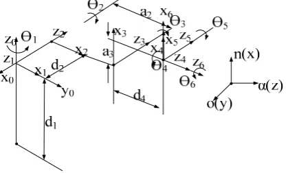
Figure 2. D-H coordinates.
overshoot is regard as one of the best indicators. Finally, this algorithm is tried in PUMA560.
The paper is organized as follows. In Section 2, the kinematics and dynamics of PUMA560 are discussed. The introduction of novel Genetic Algorithm is discussed in Section 3. In Section 4, PD ILC based on adaptive on-line tuning genetic algorithm is investiged. Finally, simulation analysis of PUMA560 trajectory control is discussed in Section 5.
II. KINEMATICS AND DYNAMICS OF PUMA560 PUMA560 is an advanced industrial robot which is produced by Unimation InC in U.S... It is a general manipulator with 6 freedom degrees including six rotatable joints. These joints are combined to mimic human waist, shoulder, elbow and wrist movements. PUMA560 is widely applied by the imitate ability. The arm can reach any point within the operating range in a
predetermined position with 6 freedom degrees. PUMA560 can perform a variety of tasks with the flexibility. So PUMA560 is an ideal research and laboratory equipment. It consists of three basic components: robots, controllers and teach pendant.
A. Kinematics
The Denavit-Hartenberg (D-H) convention is a method of drawing robot manipulators free body diagrams. Denvit-Hartenberg (D-H) convention study is necessary to calculate forward kinematics in serial robot manipulator. The coordinate system of the robot's D-H is defined as shown in Figure 1. The robot's D-H parameters are shown in Table 1[24].
End coordinates (px, py, pz) of robot arm can be calculated by the following when the angle value of each joint is known. Equations solving end coordinates (px, py, pz) follow as:
[
2 2 3 23 4 23]
2 11
a
c
a
c
d
s
d
s
c
p
x=
+
−
−
(1)[
2 2 3 23 4 23]
2 11
a
c
a
c
d
s
d
c
s
p
y=
+
−
+
(2)23 4 2 3 23
3
s
a
s
d
c
a
p
z=
−
−
−
(3)Angle value of each joint of robot arm can be calculated by the following when the end coordinates (px, py, pz) is known. Equations solving various joint variables follow as:
(
)
− ⎜⎝⎛ ± + − ⎟⎠⎞= 2
2 2 2 2
1 Atan2 py,px Atan2 d , px py d
θ (4)
(
)
− ⎜⎝⎛ ± + − ⎟⎠⎞= 2 2
4 2 3 4
3
3 Atan2a ,d Atan2 k, a d k
θ (5)
2
2 4 2 2 2 3 2 2 2 2 2
2
a
d
d
a
a
p
p
p
k
=
x+
y+
z−
−
−
−
(6)
(
)
(
)
(
)
[
(
4 23)
(
1 1)
(
2 3 3)
]
4 3 2 1 1 3 2 3
23
tan
2
,
a
c
a
p
s
p
c
p
s
a
d
d
s
a
p
s
p
c
p
c
a
a
A
y x z
y x z
+
+
+
+
−
−
+
+
−
−
=
θ
(7)
3 23
2
θ
θ
θ
=
−
(8)(
1 1 123 123 23)
4
=
A
tan
2
−
a
xs
+
a
yc
,
−
a
xc
c
−
a
ys
c
+
a
zs
θ
(9)
(
5 5)
5
=
A
tan
2
s
,
c
θ
(10)
(
6 6)
6
=
A
tan
2
s
,
c
θ
(11)
Where
s
i=
sin
θ
i,c
i=
cos
θ
i,(
i j)
ji
c
+=
cos
θ
+
θ
,s
i+j=
sin
(
θ
i+
θ
j)
.B. Dynamics
The relationship between the movement of objects and components force is described as kinetic. Newton - Euler method is used in this article. Newton - Euler equations are established based on the movement coordinates and d'Alembert.
The kinetic equations:
)
(
)
,
(
)
(
q
q
h
q
q
G
q
D
+
+
=
τ
(12)
TABLE I. D-H PARAMETER TABLE
a
i-1α
i-1d
iθ
ii
=1 0° 0 0
θ
1i
=2 -90° 0
d
2θ
2i
=3 0°
a
20
θ
3i
=4 -90°
a
3d
4θ
4i
=5 90° 0 0
θ
5For n joints of the manipulator, D(q) is the n × n positive definite matrix, which is called inertia matrix;
)
,
(
q
q
h
,is a n × 1 vector, which is called centrifugal force and the Coriolis force; G(q) is a n × 1vector of gravity.q can be calculated by the formula (13) when τ is known:
∫∫
−
−
=
D
(
q
)
−1(
h
(
q
,
q
)
G
(
q
))
q
τ
(13)
The inverse dynamics algorithm is composed of two parts: First, speed and acceleration of the link are delivery released outwardly, and then the interacting forces and moments of each link are recursive calculated inwardly, as well as joint driving force or torque.
(1) outwardly Recursion (i: 0 -> n-1) (rotating joints)
i+1
w
i+1=
i+1iR
⋅
iw
i+
θ
i+1i+1Z
i+1 (14)1 1 1 1 1 1 1 1 1 1 + + + + + + + + + + = ⋅ + ⋅ ⋅ + ⋅ i i i i i i i i i i i i i i
i w R w R w X
θ
Zθ
Z (15)[
1(
1)
]
1 1 1 + + + + +
=
+
+
i i i i i i i i i i i i i i ii
v
R
ν
w
X
P
w
X
w
X
P
(16))
(
1 11 1 1 1 1 1 1 1 1 1 1 1 + + + + + + + + + + + + + +
+
+
=
ci i i i i i ci i i i i i ci ir
X
w
X
w
r
X
w
v
ν
(17) 1 1 1 1 1 + + + + +=
ci i i cii
f
m
v
(18)
(
1)
1 1 1 1 1 1 1 1 1 1 1 + + + + + + + + + + + +
=
+
i i i ci i i i i i ci cii
n
I
w
w
X
I
w
(19)(2)inwardly Recursion (i: n-> 1)
ci i i i i i i
i
f
=
R
f
+
f
+ +
+1 1 1
(20)
1 1 1 1 1 1
1 + + + + + +
+
+
+
+
=
i i ii i i ci i ci i ci i i i i i i
i
n
R
n
n
r
X
f
P
X
R
f
(21)i i T i i i
=
n
⋅
Z
τ
(22) Note that the contact force and moment between the ends of the operating arm and the outside should be included in the equilibrium equation to be the initial value of inwardly recursive if the operating arm moves in the free space: n+1f
n+1=
n+1n
n+1=
0
. In addition,g
v
0=
0
and upward, such as the base of the robot upward accelerate with g to offset the impact of gravity if the gravity of the connecting rod is considered.
III. GENETIC ALGORITHMS
A genetic algorithm (GA) is a search technique used in computing to find true or approximate solutions to optimization and search problems, which are categorized as global search heuristics. During the last decade GAS has been applied in many engineering areas, with varying
degrees of success within each. The major elements of a typical GA for optimization of system can be synopsized with the following items:
A. Determination and Expression of the Parameters First the range of parameters generally given by users is determined; then they are coded by the accuracy requirements. Each parameter corresponds to an encoder. The relationship between the parameters and codes is established to be the object which can be operated as a genetic algorithm.
B. Selection of the Initial Population
Because of the need for programming, initial population is generated randomly by the computer. For different encoding, different forms of random numbers are resulted. In addition, the size of the population is specified by taking into account the complexity of calculation.
C. Determination of the Fitness Function
Best of the parameters meeting the conditions under constraints is selected in the general optimization design. Stability, accuracy and rapidity are considered as the indicators of a control system. The fast is reflected by the rise time. The shorter rise time, the faster control, and the better quality of the system. Fitness function related to the objective function is directly considered as a fitness function for parameter optimization when the objective function is determined.
D. Operation of Genetic Algorithm
Steps of the copy operation, the crossover operator and mutation operation are included in the specific genetic manipulation. First, fitness proportional method is used for replication. Fitness value is obtained through the fitness function, and then copy probability corresponding to each string is obtained. The product of the copy probability and string number of each generation is the number of string copied in the next generation. String of larger copy probability will have more children and grandchildren in the next generation, but the opposite will be eliminated. Secondly single-point crossover is finished with crossover probability of Pc. Matching pool is composed of string selected from member copied with probability of Pc, and then members of the matching pool are matched randomly, cross-location is determined randomly. Finally, the mutation is finished with probability of Pm. a new generation of population is obtained through reproduction, crossover and mutation of initial population. The population decoded is substituted into the fitness function until the end condition is met. End condition is determined by the specific issues, as long as the target parameter is in the specified range. The above procedure is represented in Figure 2[25-27].
Figure2. Figure of GA operation.
Figure3. Figure of the basic principle
tau q qd qdd PUMA560
Robot
In1 In2 In3 In4
OUTPUT3
In1 In2 In3 In4 In5 In6 In7 In8 In9 In10 In11 In12
Out1
Out2
Out3
Out4
Out5
Out6
OUTPUT2
In1 In2 In3 In4 In5 In6 In7 In8 In9 In10 In11 In12
OUTPUT1
Mux
Out1 Out2
INPUT
Out1 Out2 Out3 Out4 Out5 Out6
ILC
In1
In2
In3
In4 Out1
CONTROL
Figure4. Simulation platform. A. PD ILC
D type algorithm is sensitive to the high frequency interference of the error signal due to the differential action. This problem can be resolved by the P type control algorithm. The maximum error can be reduced and the tracking accuracy can be improved by PD type ILC algorithm. The conventional PD type iterative control law:
( )
t
u
( )
t
k
e
( )
t
k
e
( )
t
u
k+1=
k+
p k+1+
dk+1(
23)
Where kp and kd is the PD type iterative control gain, ek+1(t) = yd(t)- yk+1(t).
B. Adaptive On-line Tuning Genetic Algorithms
In order to improve the accuracy, PD parameters are optimized online at each sampling time with the advantage of genetic algorithm for global optimization. a sufficient number of individual is selected at sampling instant k to calculate the type of adaptation. The PD control parameters corresponding to the great degree of self- adaptive are selected as the PD control parameters at the sampling time by Genetic Algorithm optimization. In order to obtain a satisfactory transition process dynamics and prevent overshoot, absolute error and weighted and of error and error rate of change is set as the minimum objective function of parameters of the i-th individual for the k-th sampling time.
( )
i
errori
( )
i
de
( )
i
J
=
α
p+
β
p(24)
errori (i) is position self-tracking error of the i-th individual for the k-th sampling time, de(i) is rate of
position self-tracking error change of the i-th individual for the k-th sampling time.
In order to avoid overshoot, penalty function is used and overshoot is regard as one of the best indicators. Optimal index at this moment is:
If errori(i)<0
J
( )
i
=
α
perrori
( )
i
+
β
pde
( )
i
+
100
errori
( )
i
(25) Figure of the basic principle is shown in Figure3:V. SIMULATION ANALYSIS
PUMA560 is considered as the simulation object and the specific DH parameters are shown in Table 1. Six inputs and outputs are respectively qdi and qi (i = 1-6) because of six joints of PUMA560.errori (i) of J(i) is defined as:
( )
( )( )
6
6
1
∑
=
=
ji
j
error
i
2 Out2
1 Out1
z To Workspace38y To Workspace37x To Workspace36
simoutTo Workspace27 t
To Workspace
In1 In2 In3 In4 In5 In6 In7 In8 In9 In10 In11 In12
Out1
Out2
Out3
Out4
Out5
Out6
Subsystem2
slfkine S3 tau
q qd qdd PUMA560
Robot Mux
Out1 Out2 Out3 Out4 Out5 Out6
INPUT
Out1 Out2 Out3 Out4 Out5 Out6
ILC
0 Clock
Figure5. GA part.
0 0.2 0.4 0.6 0.8 1
-0.2 0 0.2 0.4 0.6
time(s)
P
o
si
ti
o
n
tr
a
cki
n
g
ideal position position tracking
(a) joint 1
0 0.2 0.4 0.6 0.8 1
-3 -2 -1 0
1x 10
-5
time(s)
P
o
si
ti
o
n
t
ra
cki
n
g
ideal position position tracking
(b) joint 2
0 0.2 0.4 0.6 0.8 1
-0.2 0 0.2 0.4 0.6
time(s)
P
os
it
ion t
rac
k
ing
ideal position position tracking
(c) joint 3
0 0.2 0.4 0.6 0.8 1
-3 -2 -1 0 1x 10
-5
time(s)
P
os
it
ion t
rac
k
ing
ideal position position tracking
(d) joint 4
0 0.2 0.4 0.6 0.8 1
-0.6 -0.4 -0.2 0 0.2
time(s)
Po
s
iti
o
n
tr
a
c
k
in
g
ideal position position tracking
(e) joint 5
( )
( )( )
6
6
1
∑
=
=
ji
j
de
i
Dei
(27)Where Errori(j)(i) is position self-tracking error of the i-th individual in the j-th size for the k-th sampling time, De(j)(i) is rate of position self-tracking error change of the i-th individual in the j-th size for the k-th sampling time.
( )
i
Errori
( )
i
De
( )
i
J
=
α
p+
β
p(28)
If errori(i)<0
( )
i Errori( )
i De( )
i Errori( )
iJ =
α
p +β
p +100 (29)The initial value of each joint is set as 0. The starting point X0 is [0.4521, -0.1505, 0.4318] and end point Xd is [0.3, 0, 0.4]. The selection of point path in this article is determined by the quaternion method. In order to facilitate the experiment, the experiment is carried out in the smart space. In the objective function, αp=0.95,
βp=0.05.In the GA part, the number of individuals Size is 120, the evolution algebra is 10, Pc is 0.9. Adaptive mutation probability method is used, that is, the greater the degree of adaptive, the smaller the mutation probability. Mutation probability Pm=0.2-[1:1: Size] ×0.01/ Size.
0 0.05 0.1 0.15
-800 -600 -400 -200 0 200 400 600 800
t/s
ui
Value of u(i)
u1 u2 u3 u4 u5 u6
Figure7. control input
0 0.2 0.4 0.6 0.8 1
-0.6 -0.4 -0.2 0 0.2
time(s)
P
o
s
it
ion
t
rac
k
ing
ideal position position tracking
(f) joint 6
Figure6. Tracking effect diagram of each joint in the different number of iterations
0 0.2 0.4 0.6 0.8 1
30 30.05 30.1 30.15
t/s
kp
Value of kp(i)
kp1 kp2 kp3 kp4 kp5 kp6
(a) kp
0 0.2 0.4 0.6 0.8 1 42
42.5 43 43.5 44
t/s
kd
Value of kd(i)
kd1 kd2 kd3 kd4 kd5 kd6
(b)kd
Figure8. kp and kd of six joints in the 20th iteration.
0 0.2 0.4 0.6 0.8 1
0.25 0.3 0.35 0.4 0.45 0.5
time(s)
P
o
s
it
ion
t
rac
k
ing
Position tracking of X
ideal position PD GA PD
(a) X direction
0 0.2 0.4 0.6 0.8 1 -0.2
-0.15 -0.1 -0.05 0
time(s)
P
os
it
ion t
rac
k
in
g
Position tracking of Y ideal position
PD GA PD
Tracking effects in 30 iterations of six joints are shown in Figure 6. It can be clearly seen that the effect gets better and better as long as more iterations. It tracks on a given trajectory basically when the number of iterations reaches to 30 times by a number of simulations.
The control inputs of the six joints are shown in Figure 7. State before 0.15s is only shown to express the change of the control input at the beginning stage well since system began to enter the stationary phase in the 0.15s time.
Change graph of kp and kd of three joints in the 30th iteration is shown in Figure8. It can obviously be seen that kp and kd change in the tracking process. It can be seen from Figure 8 that variation of kp and kd is relatively large at the beginning, because the e is relatively large and gradually stabilizes.
0 0.2 0.4 0.6 0.8 1 0.39
0.4 0.41 0.42 0.43 0.44
time(s)
P
os
it
ion t
ra
c
k
ing
Position tracking of Z
ideal position PD
GA PD
5 4 5
(c) Z direction
Figure9. Path tracking effect diagram
0 5 10 15 20 25 30
0 0.005 0.01 0.015 0.02
Change of maximum absolute value of error with times i
times
X
e
rro
r
PD GA PD
(a) X direction
0 5 10 15 20 25 30
0 0.005 0.01 0.015 0.02
Change of maximum absolute value of error with times i
times
Y
e
rro
r
PD GA PD
(b) Y direction
0 5 10 15 20 25 30 0
0.005 0.01 0.015 0.02 0.025
Change of maximum absolute value of error with times i
times
Z e
rr
o
r
PD GA PD
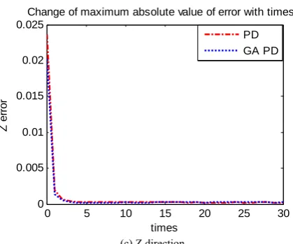
(c) Z direction
Figure10. Error convergence process in30 iterations process
Error convergence process in 30 iterations is shown in Figure 10. It can be seen that convergence rate in PD iterative self-learning control proposed is better than PD iterative control whether in the X direction or Y direction, as well as the final error value is smaller.
VI. CONCLUSION
PD iterative control based on adaptive on-line genetic algorithm of PUMA560 is researched in depth. The basic principle of genetic algorithm and the PD type iterative learning control is understood firstly. Then an online adaptive PD iterative learning control algorithm is proposed. PD parameters are optimized online at each sampling time with the advantage of genetic algorithm for global optimization. In order to avoid overshoot, penalty function is used and overshoot is regard as one of the best indicators. Simulation analysis shows that the proposed algorithm is better than unmodified in accuracy. But, this algorithm only applies to industrial robots of less rapid demanding and is referenced for further study of the repetitive motion trajectory tracking control for industrial robots of higher rapid demanding.
REFERENCES
[1] S. Arimoto, S. Kawamura, and F. Miyazaki, “Betering operation of robots by learning,” Journal of Robotic Systems, vol. 1, pp. 123-140, 1984.
[2] O. Purwina, D. A. Raffaello, “Performing and extending aggressive maneuvers using iterative 1earning control,” Robotics and Autonomous Systems, vol. 59, pp. 1-11, 2011.
[3] B.Depraetere, G. Pinte, and W. SYMENS, “A two-1evel Iterative Learning Control scheme for the engagement of wet clutches,” Mechatronics, vol. 2l, pp. 501-508, 2011. [4] S.R. Oh, Z. Bien, I. Suh,, “An iterative learning control
method with application for the robot manipulator,” IEEE Journal of Robot and Automation, vol. 4, pp. 508-514. [5] K. L. Moore, M. Daheh, and S. P. Bhattacharyya,
“Iterative learning control: A Survey and New Results,” Journal of Robotic Systems, vol. 9, pp. 536-594, 1988. [6] H. S. Ahn, Y. Q. Chen, and L. Kevin, “Iterative Learning
Control: Brief Survey and Categorization,” IEEE Transactions on systems, man, and cybernetics-part c: applications and reviews, vol. 37, 2007.
[7] Z. J. Feng, “Open closed loop PD-type iterative learning control and its convergence,” Master Thesis, Hangzhou: Zhejiang University; 2005..
with random disturbance,” Telkomnika, vol. 11, pp. 443-448, 2013.
[9] X. Y. Li, Y. Xu, Y. Wang, “Improved PD-type iterative learning control algorithm of time-invariant system,” Engineering and Applications, vol. 44, pp. 75-78, 2008. [10]D. Pawel, G. Krzysztof, R. Eric, Z. L. Cai, C. T. Freeman,
and L. L. Paul, “Iterative Learning Control Based on Relaxed 2-D Systems Stability Criteria,” IEEE Transactions on control systems technology, vol. 21, 2013. [11]N. Amaon, D. Owens and E. Rogers, “Predictive optimal
iterative learning control”, INT Journal of Control, vol. 69, pp. 203-226, 1998.
[12]V. Hatzikos, D. Owens, “A Genetic Algorithm Based Optimization Method for Iterative Learning Control Systems,” Third International Workshop on Robot Motion and Control, 2002.
[13]N. Amaon, D. Owens, E. Rogers. “Iterative Learning control using optimal feedback and feed forward actions,” INT. Journal of Control, 1996.
[14] T. Tao, R.L. Kosut and G. Aral, “Learning feed forward control,” Proc of ACC, pp. 2575-2579, 1994.
[15]C. T. Freeman, “Constrained point-to-point iterative learning control with experimental verification,” Control Engineering Practice, vol. 20, pp. 489-498, 2012.
[16]D. Q. Huang, J. X. Xu, “Steady-state iterative learning control for a class of nonlinear PDE processes,” Journal of Process Control, vol. 21, pp. 1155–1163, 2011.
[17]C. C. Lee, “Fuzzy logic in control systems: Fuzzy logic controller-partI and II,” IEEE Trans. Syst., Man, Cybern., vol. 20, pp. 404–435, Apr.1990.
[18]K. S. Narendra and K. Parthasarathy, “Identification and control of dynamical system using neural networks,” IEEE Trans. Neural Networks, vol. 1, pp. 4–27, 1990.
[19]H. S. Ahn, Y. Q. Chen and K. L. Moore, “Iterative learning control: brief survey and categorization,” IEEE Transactions on Systems, Man and Cybernetics Part C: Applications and Reviews, vol. 37, pp. 1099–1121, 2007. [20] D.A. Bristow, M. Tharayil, and A.G. Alleyne, “A survey
of iterative learning control: a learning-based method for
high-performance tracking control,” IEEE Control Systems Magazine, vol. 26, pp. 96–114, 2006.
[21]T. D. Sona, H. S. Ahna, and K. L. Mooreb, “Iterative learning control in optimal tracking problems with specified data points,” Automatica, vol. 49, pp. 1465–1472, 2013.
[22]V. Hatzikos, J. Hatonen, D. H. Owens, “Genetic algorithms in norm—optimal linear and non—linear iterative learning control,” International Journal of control, vol. 77, pp. 188—197, 2004.
[23]D. H. Nguyena, B. David, “A convex optimization approach to robust iterative learning control for linear systems with time-varying parametric uncertainties,” Automatica, vol. 47, pp. 2039–2043, 2011.
[24]Y. L. Xiong, “Robot technology base”, Huazhong University of Science & Technology Press, Wuhan, 1996. [25]J. K. Liu, “MATLAB simulation of Advanced PID
control”, Bei Jing: Publishing House of Electronics Industry. 2011.
[26]E. H. Sue, G. S. Young, C. T. Allen, “A Genetic Algorithm Method to Assimilate Sensor Data for a Toxic Contaminant Release, ” Journal Of Computers, vol. 2, pp.85-93, 2007.
[27]C. G. Xue, L. L. Dong, “An Improved Immune Genetic Algorithm for the Optimization of Enterprise Information System based on Time Property,” Journal Of Software, vol. 6, pp.436-443, 2011.