An improved artificial fish swarm algorithm for optimal operation of cascade reservoirs

An improved artificial fish swarm algorithm for

optimal operation of cascade reservoirs

Yong PENG

Hydraulic Engineering Institute, Dalian University of Technology, Dalian, China Email: [email protected]

Abstract—Based on traditional artificial fish swarm algorithm (AFSA), an improved artificial fish swarm algorithm (IAFSA) is proposed and used to solve the problem of optimal operation of cascade reservoirs. To improve the ability of searching the global and the local extremum, the vision and the step of artificial fish are adjusted dynamicly in IAFSA. Moreover, to increase the convergence speed, the threshold selection strategy is employed to decrease the individual large space gap between before and after update operation in the local update operation. The validity of IAFSA is proved by case study and the threshold parameters of IAFSA are rated.

Index Terms—Reservoir operation, Optimization, Hydroelectric power generation

I. INTRODUCTION

Under the call of energy conservation, renewable resources, such as hydropower, wind power, biomass power and garbage power, have become the priority to be utilized to participate in the operation of electric power. Furthermore, this idea encourages generating more power by hydropower and requires improving the utilization ratio of the hydropower. Consequently, high requirements are also put forward to the optimization operation of reservoirs. How to perform the optimization operation of reservoirs and utilize the water power resource effectively has become a hot issue.

The optimization operation of cascade reservoirs, a complex mathematical optimization control problem of a nonlinear dynamic system with a large number of constraints, has been drawn much attention to many researchers. So far there are many traditional algorithms, such as linear programming [1], nonlinear programming [2], network flow programming [3], dynamic programming [4], and lagrangian relaxation [5], etc., have been used for the optimization operation of cascade reservoirs. However, these algorithms have the disadvantages of dimensionality curse, unstable convergence or complexity and so on. Nowadays, some intelligent optimization algorithms have been successfully applied, such as tabu search algorithm [6], simulated annealing algorithm [7], genetic algorithm [8], ant colony algorithm [9] and particle swarm optimization algorithm [10], etc.

Artificial fish swarm algorithm (AFSA) is a novel method for searching the global optimum, which is

typical application of behaviorism in artificial intelligence [11]. It is a random search algorithm based on simulating fish swarm behaviors which contains preying behavior, swarming behavior and following behavior. It constructs the simple bottom behaviors of artificial fish (AF) firstly, and then makes the global optimum appear finally based on animal individuals’ local searching behaviors. This algorithm has strong ability of avoiding the local extremum and achieving the global extremum, its usage is flexible and convergence speed is fast. It doesn’t need the characteristics such as the grads value of objective function, thus it has a certain adaptive ability for search space, which belongs to swarm intelligence algorithm essentially.

However, this algorithm has several disadvantages such as the blindness of searching at the later stage and the poor ability to keep the balance of exploration and exploitation, which reduce its probability of searching the best result. In this paper, an improved AFSA (IAFSA) is proposed to overcome these defects. The improved algorithm can adjust the search range adaptively and have better ability to keep the balance of exploration and exploitation. To verify the effectiveness of IAFSA for obtaining reservoir operating polices, IAFSA is applied to a cascade reservoirs system, namely the Baishan-Fengman reservoirs system in Jilin province, China.

II. MATHEMATICAL MODEL FOR THE OPTIMIZATION OPERATION OF CASCADE RESERVOIRS

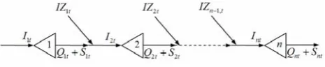
According to the inflow process, the optimization operation of cascade reservoirs takes the power discharges as the decision variables, and takes the maximal gross power generation in one scheduling period as the target. Suppose there are n hydropower stations in cascade power stations, as shown in Fig.1.

Figure 1. The sketch of cascade power stations

A. Objective function:

} ) (

3600 max{ max

1 1

∑∑

⋅ ⋅

= n

p T

t

pt t

pt M R

Q

Where, E is the gross power generation of cascade

power stations; Q_pt is the power discharge of power station p in interval t; Mt is the number of hours in

interval t; R_pt is the mean water rate of power station p in interval t, its unit is m3/kW·h; n is the number of the reservoirs; T is total time-interval for calculation. B. Constraints:

Water balance equations constraint t S Q I V

Vp,t+1= pt+( pt− pt− pt)Δ (2)

Storage capacity constraint min

pt

V ≤Vpt≤Vptmax (3) Correlation equation

pt pt pt t

p Q S IZ

I _+1, = + + ；I_1t =IZ_1t (4) Turbine discharge constraint

min

pt

Q ≤Qpt≤Qptmax (5) Spillway capacity constraint

0≤Spt≤Sptmax (6) Boundary constraint

1

p

V =Vp1c；Vp,T+1=Vp,T+1,c (7)

Outflow from reservoir constraint min

pt

q ≤Qpt+Spt≤qptmax (8) Output of power station constraint

min

p

N ≤3600⋅Qpt Rpt ≤Npmax (9) Relationship between water level and storage capacity

Vpt =Up(Zpt) (10) Where, Vp,t+1 is the storage capacity at the end of the interval t; V_pt is the storage capacity at the beginning of the interval t; I_pt is the mean inflow of reservoir p in interval t ; Spt is the surplus water of reservoir p in

interval t; S_ptmax is the spillway capacity of reservoir p in interval t; Δt is the duration of interval t; V_ptmin is the required minimal storage capacity of reservoir p at the beginning of interval t ; Vpt_max is the permissible

maximal storage capacity of reservoir p at the beginning of interval t; Qptmin is the minimal power discharge of power station p in interval t ;Qptmax is the maximal power discharge of power station p in interval t . Considering the power discharge of cascade reservoirs and the agricultural and industrial water-supply in downstream, when Qpt < Qptmax , Spt = 0. While

pt

Q =Qptmax, Spt≥0. Vp1c and Vp,T+1,c are the storage

capacity of reservoir p at the beginning and at the end of the optimization scheduling period, respectively. qptmin is the minimal water discharge of reservoir p in interval t;

max

pt

q is the safety discharge at lower river in interval t; min

p

N is the minimal output of power station p; Np_max

is the maximal output limit of power station p; Zpt is

the water level of reservoir p at the beginning of interval t; Up represents the function of the relationship between

the water level and the storage capacity of reservoir p. In the optimization operation model of cascade power stations mentioned above, the objective function is used to obtain the maximal gross power generation under the decision variables Q11, Q12, …, QnT , which is a n⋅T

-dimension vector. Since the power discharge Qpt is the

implicit function of the water level Z_pt, the problem can be transformed into getting the maximal gross power generation under Z11，Z12，…，ZnT .

The constraints, which are difficult to be reckoned in feasible region, can be expressed by using penalty function. Then the objective function can be expressed as follows

∑

+ − = −

= l

l l i

i Z

h Z

E Z

F

1 2 1

0

)) ( ( )

( max{ ) (

max σ

} )}] ( , 0 [max{

1

2 2

0

∑

−

− u

u u j

j Z

g

σ (11)

s.t. hi(Z)=0， i=1,2,...,l−l0 )

(Z

gj ≥0， j=1,2,...,u−u0

Where, E(Z) is the original objective function. )

,..., ,

(Z11 Z12 ZnT

Z = T is a n⋅T-dimension vector. l, u

is the number of equality and inequality constraints. σ1 and σ2 are penalty factors. The feasible region of Eq.(11) can be written as follows

; ,..., 2 , 1 , 0 ) ( |

{Z h Z i l l₀

Scope= i = = −

} ,..., 2 , 1 , 0 )

(Z j u u0

gj ≥ = − (12)

III. AFSAAND IAFSA

AFSA, a new population-based evolutionary computation technique inspired by the natural social behavior of fish schooling and swarm intelligence was first proposed in 2002 [11].

A. Principle of AFSA

(1) Preying behavior: This is a basic biological behavior that tends to the food. Generally fish perceives the concentration of food in water by vision or sense to determine the movement and then chooses the tendency.

(2) Swarming behavior: Fish will assemble in groups naturally in moving process, which is a kind of living habits to guarantee the existence of the colony and avoid dangers. While swarming, they obey the following three principles: ① Compartmentation principle: to avoid congestion with other fellows. ②Unification principle: to move approximately toward other fellows’ average moving direction. ③ Cohesion principle: to move approximately toward the center of near fellows.

(3) Following behavior: In moving process of the fish swarm, when a single fish or several ones find food, the neighborhood fellows will trail and reach the food quickly.

In AFSA, the food consistence in water is defined as the objective function, and the state of an AF is the variable to be optimized. Preying behavior is that AF moves randomly according to its fitness value, thus it is an optimization of individual extremum and belongs to self-studying process; it keeps the diversity of colony. Swarming behavior and following behavior are processes of AF interaction with surrounding environment. These two processes can ensure that it will not be too crowded for an AF with other fellows and the moving direction of AF is consistent with the average moving direction of other near fellows which are moving towards the colony extreme, the convergence of colony can be kept. Therefore, AFSA is also one optimization method based on swarm intelligence. After doing the above mentioned behaviors, AF gets to the place where food consistence is the biggest. During the whole optimization process of AFSA, self-information and environment information are fully used to adjust the search direction to achieve the balance of diversity and convergence.

B. Description of AFSA

In AFSA, AF model based on behaviors is constructed by multiple parallel pathways architecture, and this model encapsulates the self-state and the behavior of AF. The process of algorithm is the self-adaptive behavior of AF. The algorithm iterates once means AF moves once.

(1) Structure of AFSA and definitions

Suppose that the search space is D-dimensional and m fish form the colony. The state of AF can be expressed by vector X =(x1,x2,",xD) , where

i

x (i=1,2,"D) is the variable to be searched for the optimal value; the food consistence at present position of AF can be represented by Y = f(X), and Y is the

objective function; the distance between AFs can be expressed as di,j = xi−xj ; Visual represents the vision

distance; Step is the maximal step length and δ is the crowd factor.

The key of the optimization operation of cascade reservoirs based on AFSA lies in the structure of AF

model. According to the above definition and mathematical model for the optimization operation of cascade reservoirs, the state of AF can be expressed with vector X=(Z11, Z12, …, ZnT ), the distance between AFs

can be expressed as:

2 / 1

1 1

2 )

( ⎥

⎦ ⎤ ⎢

⎣ ⎡

− =

∑∑

= =

n

p T

t

j pt i pt

ij Z Z

d ,

and the food consistence at present position of AF can be represented by Eq. (1).

(2) Description of the behaviors ① Preying behavior

Suppose that an AF's current state is Xi. We randomly

select a new state Xj in its visual field. If Yi <Yj in the

maximum problem, it goes forward a step in this direction; otherwise, select a state Xj randomly again

and judge whether it satisfies the forward condition. If it can't satisfy after try_number times, it moves a step randomly. When the try_number is small in preying behavior, AF can swim randomly, which makes it flee from the local extreme value field. The pseudocode is as follows:

float Artificial_fish::prey() {

isChange=true;

for (i=0;i<try_number;i++) {

Visual Random

X

X_j = _i+[ (1)×2−1]× ; if (Yi <Yj)

; ]

1 2 ) 1 ( [

i j

i j i

next i

X X

X X Step Random

X X

− − × × − × +

= (13)

isChange=false;break; }

if(isChange)

; ] 1 2 ) 1 (

[Random Step

X

X_inext = _i+ × − × (14)

}

② Swarming behavior

An AF with the current state Xi seeks the fellow's

number in its current neighborhood where satisfy

Visable

d_i,j < ; and calculate their center position X_c, Y_c denotes the food consistence of the center position and

f

n denotes the number of fellows of Xi in the near

fields, if nf ≥1, Xj explores the center position of its

fellow. If Yc/nf >δYi , which means that the food

behavior. If nf =0, AF executes the preying behavior.

The pseudocode is as follows: float Artificial_fish::swarm() {

; 0 ;

0 =

= _c

f X

n

for ( j=0; j<m; j++ )

if (di,j <Visable) {nf ++;Xc+=Xj;} if(nf =0) prey();

else{

Xc =Xc/nf; if (Yc/nf >δYi)

; )

(

i c

i c i

next i

X X

X X Step Random X

X

− − ⋅ +

= (15)

else

prey();

} }

③ Following behavior

An AF with the current state Xi seeks the fellow's

number in its current neighborhood where satisfy

Visable

d_i,j < , and find the maximal positionX_max, Y_max

is the maximal value of its fellows in the near fields and

f

n denote the number of fellows of Xmax in the near fields. If n_f =0 or Yc/nf >δYi, which means that the

fellow Xmax has high food consistence and the surrounding is not very crowded, forward a step to the fellowXmax. Otherwise AF executes the preying behavior. The pseudocode is as follows:

float Artificial_fish::follow() {

; 0 ; max =−∞ nf =

Y

for ( j=0; j<m; j++ )

if (d_i,j <Visable && Y_j >Y_max) {Ymax =Yj;Xmax =Xj;}

for ( j=0; j<m; j++ ) if(dmax,j <Visual) nf ++; if (nf =0 or Ymax/nf >δYi)

; )

(

max max

i i i

next i

X X

X X Step Random X

X

− − ⋅ +

= (16)

else

prey(); }

(3) Selection of the behaviors

The behavior of X_i(iter)(iteris the current iterative number) is determined by the hunger degree of AF. Here, the hunger degree is represented by energy. If the energy of Xi(iter) is lower than

∑

⋅ = m

i

i iter

Y m iter Energy

1 ) ( 1 ) (

AF takes the following behavior to get food in the area with high food consistence to obtain energy; If the energy of X_i(iter) is higher than Energy(iter) , AF is not

hunger, thus it chooses the swarming behavior to avoid harmful animals. If AF takes the following behavior and the swarming behavior unsuccessfully, it will execute the preying behavior.

(4) Bulletin

Bulletin is used to record the optimal state and the food consistence at present position of AF. Update the bulletin with the better state of AF, the final value of the bulletin is the optimal value of the problem, the state of which is the optimal solution of the system.

C. Improved AFSA

(1) Improvement of Visual and Step

The AFSA demonstrate that Visual has great influence on the three behaviors and the convergence of the algorithm. When Visual is larger, AF has strong global search ability and fast convergence speed; and when Visual is smaller, AF has strong local search ability. The bigger the Step is, the faster the convergence will be, though the oscillation sometimes appears; In contrast, the smaller the Step is, the slower the convergence will be, whereas the solving accuracy is higher.

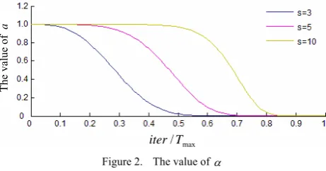
According to the above mentioned, the more difficultly a function is optimized, the more the global search ability of this function should be improved. Moreover, after the position of the optimal solution is allocated, the local search ability also should be improved. Therefore, to improve the global search ability and the convergence speed of AFSA, larger Visualand larger Step are taken in prior period to make AF search in a larger scope in IAFSA. With the searching proceeds, Visual and Step decrease gradually, then the local search carries out in adjacent domain of the optimal solution, which consequently increases the local search ability and the solving accuracy of the algorithm. In this improved algorithm, Visual and Step are adjusted dynamically by following equations:

⎪ ⎪ ⎪ ⎩ ⎪⎪ ⎪ ⎨ ⎧

× − =

+ × =

+ × =

) ) / ( 30

exp( max

min min

s

T iter

Step Step

Step

Visual Visual

Visual

α

α α

(17)

Visual is the maximum of the search scope. Visual and Step and are piecewise functions, which keep maximum in prior period, then decease gradually, finally keep minimum. The value of α is Show in Fig.2.

Figure 2. The value of α

(2) Improvement of update operation

In AFSA, When the algorithm carries out update operationto each fish, the component in each dimension of X_i will be processed randomly by Eq. (13) ~ (16),

which makes the position of Xi change greater after

update operation. With increasing of the dimensions, the position change of Xi increases. Therefore, though this

update operationcan enlarge the search scope of solution space, the global optimal solution will be easily skipped, which decreases the rapidity of convergence and accordingly increase the calculation time.

Therefore, to reduce the individual large space gap between before and after update operation, an improvement based on threshold selection strategy is conducted in IAFSA. The basic idea of this strategy is that during update operation of the component of Xi in

dimension j by Eq. (13) ~ (16), a random criterion is

introduced: When the random value is not larger than the threshold q0, the moving distance of the component in dimension j is determined by Eq. (13) ~ (16); When the

random value is larger than the threshold q0 , the component of Xi in dimension j is not changed. This

strategy can decrease the space gap between before and after update operation of X_i , which is good for fast

convergence. D. Steps of IAFSA

The steps of the optimization operation of cascade reservoirs based on IAFSA are as follows:

(1) Initialization of the parameters: The number of AF is m, the scope of vision is Visual, Visualmin , the maximum of moving step length is Step, Stepmin, crowd factor is δ , the maximal try number is try_number, the threshold value is q0, the maximal iterative number is

max

T .

(2) Initialization of the position vectors of the swarm: For operation problem of cascade reservoirs, the search space is equal to the total number of release combinations. Each decision variable represents a parameter to be optimized in the model. The initial positions of all AF

have to be generated randomly within the limit specified for each decision variable. Moreover, the initial search points are the initial random release values. In this step, each AF vector represents one operation process of the cascade reservoirs, and the water level at each interval is denoted by the coordinates of the AF vectors. Set initial iterative number iter=0.

(3) Initial evaluation of the fitness function: Calculate the food consistence of initial AF Y and compare them,

then put the biggest food consistence into the bulletin, and conserve the state and the value of Y.

(4) Calculate Visual and Step by Eq. (17).

(5) AF executes the swarming behavior, the following behavior, or the preying behavior according to its energy.

(6) Checks the state and the bulletin. If the self-state is superior to the bulletin, then the bulletin is replaced.

(7) Judge the terminate condition: If the iterative number reaches the maximal iterative number Tmax, then output the result (the value of bulletin). Otherwise, execute iter=iter+1, and turn to step (4).

IV. GENERATION OF INITIAL AFSWARM AND THE FEASIBLE REGION

The detail procedures of the generation of initial AF are as follows:

(1) Considering the influence of Qpt on Spt, the value

range of Qpt is determined firstly: Upper bound:

} )

( ,

min{Qptmax Vpt−Vp,t+1,min Δt+Ipt (18) Lower bound:

} )

( ,

max{Qptmin Vpt−Vp,t+1,max Δt+Ipt (19)

If “Upper bound” < “Lower bound”, let “Upper bound” = “Lower bound”=Qptmax, then generate an initial

0

pt

Q of Q_pt randomly in this value range.

(2) Determine the value range of Spt: Upper bound:

} )

( ,

min{ 0

min , 1 ,

max pt pt pt pt

pt V V t I Q

S − ₊ Δ + − (20)

Lower bound:

} )

( ,

max{ 0

max , 1 ,

min pt pt pt pt

pt V V t I Q

S − ₊ Δ + − (21)

Then generate an initial 0

pt

S of S_pt randomly in the

value range.

(3) Determine the initial value of Vp_,t₊₁ after obtaining

the initial value of Q_pt和Spt, that is

t S Q I V

V_p0_,t+1 = _pt+( _pt− _pt0 − _pt0)Δ (22)

Each AF obtains the variation process of the initial storage capacity like above mentioned, and then the initial AF swarm can be obtained accordingly. The initial max

/T iter

The value of

AF swarm must satisfy the water balance Eq.(2) and the corresponding constraints Eq.(3) ~ (6), which make each AF of the initial AF swarm in the feasible region and accelerate the convergence.

The initial AF swarm satisfies Eq. (7) Vp₁=Vp1c, but it

does not always satisfies the ending condition 1

,T+

p

V =Vp,T+1,c. Without regard to the ending condition,

large numbers of the pilot calculation are carried out for the model. The results show that, to obtain the maximum electric benefit, the model is inclined to use all the water generate electricity, which is likely to make the water level minimum at the terminal stage of the calculation. According to this characteristic, the ending condition is changed into inequation, i.e. Vp,T+1≥Vp,T+1,c. Here, the

initial AF swarm also satisfies Eq. (7).

Based on the above mentioned, when inequation (8) and inequation (9) are difficult to be reckoned in Eq.(11), the feasible region can be express as

{

=

Scope V_p,t+1 =V_pt+(I_pt−Q_pt−S_pt)Δt;

min

pt

V ≤Vpt≤Vptmax; Qptmin≤Qpt≤Qptmax; 0≤Spt≤Sptmax; 1

p

V =V_p1c; V_p,T+1≥V_p,T+1,c} (23)

V. CASE STUDY

Baishan reservoir and Fengman reservoir are all have the function of seasonal regulation. Banshan reservoir is in the upstream of Fengman reservoir and there is a local inflow into Fengman reservoir. The dead water level, the normal water level, the limited water level and the maximal permissible storage water level at post-freshet period of Baishan reservoir are 380m, 413m, 413m and 416m, respectively. And the maximal water discharge of Baishan reservoir is 1500m3_{/s, the firm output is} 16.7×104_{kW, the maximal power output is 155×10}4_kW. For Fengman reservoir, the dead water level, the normal water level, the limited water level and the maximal permissible storage water level at post-freshet period are 242m, 261m, 261m and 263.5m, respectively. And the maximal water discharge of Fengman reservoir is 1126.5m3_{/s, the firm output is 16.6×10}4_{kW, the maximal} power output is 60.25×104_{kW. To ensure the safety of} these two reservoirs, it is needed that the water levels in July and August must be lower than the limited water level. And these two reservoirs are permitted over storage to the maximal permissible storage water level at post-freshet period after September. In view of multipurpose use, Fengman reservoir also supplies the water at the discharge of 120 m3_{/s to agricultural irrigation,} navigation and industry.

A. Performance test of IAFSA

The inflow process of Baishan-Fengman cascade reservoirs from 1987 to 1988 are used to validate the effectiveness of IAFSA. The initial water level and the termination water level of each reservoir are all the dead water level; the minimal output of each hydropower station is the firm capacity; the calculation interval is defined as month, that is T=12. During the calculation,

P4-1.6G personal computer is used. Its memory size is 512M, the operation system is WinXP, and the algorithm is realized by Java.

The parameters of the IAFSA: The number of AF m=50, Visual=40, Visual_min=0.4, Step=0.4, Step_min=0.1,

δ =0.618, try_number=4, q0 =0.07, Tmax =1000. The termination criterion is defined as follows: the absolute value of the difference between two adjacent iterations of 50 iterations is less than 10×104_{kW·h. To avoid the} accidental circumstance, 100 times simulations have been done, then the average value is obtained. The optimization operation result is shown in TableI.

TABLE I. COMPARISON OF THE RESULTS OF DIFFERENT MODELS IN YEAR 1987-1988

AFSA IAFSA PSO DP

Power generation

(×104_kW·h) 477932 485020 484572 488605

Calculation time 7.1s 6.2s 6.7s 8.4h

To demonstrate the validity of IAFSA, comparison has been done between it and traditional DP algorithm[12], which is shown in TableI. For traditional DP algorithm, the number of the discrete points of two reservoirs are all 200, the total power generation is 488605×104_{kW·h. The} average power generation of IAFSA under 100 times simulations is 485020×104kW·h, which has a difference of 0.73% with that of DP. The difference can be accepted. Furthermore, IAFSA increases the solution speed greatly and there is no curse of dimensionality. The calculation time of DP with 200 discrete points is 8.4 hours, and the average calculation time of IAFSA under 100 times simulations is only 6.2 seconds.

B. Rating of the threshold

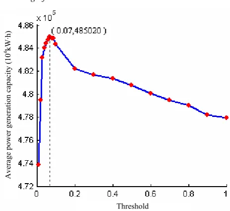
Figure 3. Relationship between the average power generation capacity and the threshold

Threshold

Average power ge

neration capacity (

10

4kW·

Fig.3 shows the average power generation capacity under different thresholds. From this figure, it can be seen that the maximum generating capacity can be found by IAFSA when the threshold is between 0.06 and 0.09. And the recommended value of the threshold q₀is 0.07.

C. Further performance test of IAFSA

To further verify the efficiency of IAFSA for the optimization operation of the cascade reservoirs, the power generation dispatching of the cascade reservoirs from 1986 to 1987 are performed in this paper. TableII lists the results of IAFSA and DP, respectively. Comparing the results between IAFSA and DP, it is found that for DP, when the number of the discrete points of two reservoirs are all 200, the power generation capacity is 642843×104_{kW·h; For IAFSA, the average} power generation capacity under 100 times simulations is 640568×104_{kW·h. The difference between IAFSA and} DP is 0.35% , which can be accepted.

TABLE II. COMPARISON OF THE RESULTS OF DIFFERENT MODELS IN YEAR 1986-1987

AFSA IAFSA PSO DP

Power generation

(×104_kW·h) 634032 640568 637905 642843

Calculation time 5.7s 5.1s 5.5s 7.9h

VI. CONCLUSIONS

Aiming at the disadvantages of AFSA, such as the blindness of searching at the later stage and the poor ability to keep the balance of exploration and exploitation, etc., an improved AFSA (IAFSA) suitable for optimization operation of cascade reservoirs is proposed. The results demonstrate that the capability of IAFSA has greater improvement than that of AFSA and the optimization operation resultsofIAFSA are satisfied.

ACKNOWLEDGEMENTS

This research is supported by “Specialized Research Fund for the Doctoral Program of Higher Education” (20100041120004), “Open Research Fund of State Key Laboratory of Hydrology-Water Resources and Hydraulic Engineering, Hohai University” (2009490211), “the Fundamental Research Funds for the Central Universities” (1100-893345).

REFERENCES

[1] Shawwash, Z. K., Siu, T. K. and Russell, S. O. D , “The

B.C. Hydro Short Term Hydro Scheduling Optimization

Model,” IEEE Transactions on Power Systems, vol. 15, pp.

1125-1131, 2000.

[2] Xiaohong Guan, Luh, P. B. and Lan Zhang, “Nonlinear

approximation method in Lagrangian

relaxation-basedalgorithms for hydrothermal scheduling,” IEEE

Transactions on Power Systems, vol. 10, pp. 772-778, 1995.

[3] Franco, P. E. C., Carvalho, M. F. and Soares, S, “A

Network Flow Model for Short-term Hydro-dominated

Hydrothermal Scheduling Problems,” IEEE Transactions

on Power Systems, vol. 9, pp. 1016-1022, 1994.

[4] Yang Jin-Shyr and Chen Nanming, “Short Term

Hydrothermal Coordination Using Multi-pass Dynamic

Programming, ” IEEE Transactions on Power Systems, vol.

4, pp.1050-1056, 1989.

[5] Zhuang F and Galiana F D, “Towards a more rigorous and

practical unit commitment by Lagrangian relaxation,”

IEEE Transactions on Power Systems, vol. 3, pp. 763-773,

1988.

[6] Xaiomin Bai and Shahidehpour, S. M, “Hydro-thermal,

scheduling by tabu search and decomposition method,”

IEEE Transactions on Power Systems, vol. 11, pp. 96-974,

1996.

[7] Ramesh S. V. Teegavarapu and Slobodan P. Simonovic,

“Optimal Operation of Reservoir Systems using Simulated

Annealing,” Water Resources Management, vol. 16, pp.

401-428, 2002.

[8] Wardlaw, R., and Sharif, M, “Evaluation of genetic

algorithms for optimal reservoir system operation,” J.

Water Resour. Plann. Manage., vol. 125, pp. 25–33, 1999.

[9] D. Nagesh Kumar and M. Janga Reddy, “Ant Colony

Optimization for Multi-Purpose Reservoir Operation,”

Water Resources Management, vol. 20, pp. 879-898, 2006.

[10]D. Nagesh Kumar and M. Janga Reddy, “Multipurpose

Reservoir Operation Using Particle Swarm Optimization,”

J. Water Resour. Plann. Manage., vol. 133, pp. 192-201,

2007.

[11]LI Xiao lei, SHAO Zhi-jiang and QIAN Ji-xin, “An

optimizing method based on autonomous animals:

fish-swarm algorithm,” Systems Engineering Theory &

Practice, vol. 22, pp. 32-38, 2002.

[12]PENG Yong, Liang Guo-hua, ZHOU Hui Cheng, “Optimal

operation of cascade reservoirs based on improved particle

swarm optimization algorithm,” Journal of Hydroelectric

Engineering, vol. 28, pp. 49-55, 2009.

Yong PENG. The author was born in

Hubei province, 1979. In 2007, the author graduated from School of Civil and Hydrolic Engineering, Dalian University of Technology and earned the doctor degree. The author’s major field of study is water resource and flood control.

He is the lecturer of Dalian University of Technology. Current research interest is multi-purpose optimization of water resource system and decision support system of flood control. Represent aritcle is:

[1] Zhou Hui-cheng, Peng Yong, Liang Guo-Hua, “The

research of monthly discharge predictor-corrector model

based on wavelet decomposition,” Water Resources

Management, 2008.

[2] Peng Yong, Liang Guo-hua, “Fuzzy Optimization Neural

Network Model Using Second Order Information,”

FSKD'09, 2009.

[3] Peng Yong, Wang Guo-li, He Bin, “Optimal Operation of

Cascade Reservoirs Based on Generalized Ant Colony

Optimization Method,” ICNC2010, 2010.

[4] Peng Yong, Xue Zhi-chun, “Research of long-term runoff

forecast based on support vector machine method,”