Evaluation of Detrending Method Based on Ensemble Empirical Mode Decomposition for HRV Analysis

Evaluation of Detrending Method Based on

Ensemble Empirical Mode Decomposition for

HRV Analysis

Chao Zeng1, 2

1 _{School of Geosciences and Info-physics, Central South University, Changsha, Hunan, 410083, China} 2_{College of Information Science and Technology, Shihezi University, Shihezi, 832003,China}

Email: [email protected]

Xiaowen Xu1*

*1 _{School of Geosciences and Info-physics, Central South University, Changsha, Hunan, 410083, China} Email: [email protected]

Abstract—Heart rate variability (HRV) is a key indicator for assessing autonomous nervous system activity. Because nonstationary and slow trends which can cause distortion to HRV analysis are usually occurred in HRV signals, detrending scheme is necessary before HRV analysis. Ensemble empirical mode decomposition (EEMD), which offers the ability to break down signals into a set of intrinsic mode functions and acts as a high-pass filter through partial reconstruction, is proposed for HRV detrending. Experiment results show that the detrending method based on EEMD can achieve better performance than the smoothing priors approach (SPA), which is one of the most widely used method.

Index Terms—Ensemble Empirical Mode Decomposition; Heart Rate Varibility; Detrending; Smoothing Priors Approach

I. INTRODUCTION

The variation of time interval between heart beats, which is usually determined by the consecutive RR intervals of ECG recordings, is known as heart rate variability. As it reflects the function of the automatic nervous system, HRV has attracted much attention in biomedical and clinical research during the past few decades [1-2]. Consequently, a number of methods, such as time domain, frequent domain and nonlinear methods have been proposed to quantify the fluctuation in heart rate [1]. However, the slow linear or more complex trends in HRV signals will affect significantly the accuracy of analysis results. To obtain reliable results of HRV analysis, it is essential to extract the trends in HRV signals and remove them by subtraction before analysis [3-5].

Several methods have been proposed to deal with the

problem of the extraction of trends which is usually considered to be nonstationary [6]. Fist-order [7, 8]and higher order [8] polynomial models have been used before analysing HRV. The polynomial filter is very sensitive to the choice of polynomial order and the duration [9]. To avoid these problems the Smoothness prior approach (SPA) was purposed [6], it is more widely adopted [3, 5, 10] in HRV analysis. The SPA acts as a time-varying finite impulse high-pass filter and addresses directly the phenomenon of nonstationarity [10]. The effects of SPA on linear and nonlinear analysis of HRV in estimation of the depth of anesthesia have been studied in [3].

Empirical mode decomposition, introduced by Huang et al [11], provided new insight in nonlinear and nonstationary signals. The method locally decomposes signals into oscillating components, which are called intrinsic mode functions (IMFs). Due to its properties of adaptive and fully-data driven, it is very attractive in the biomedical signal processing filed. Its ability for removing the baseline wander in ECG [12] and detrending in HRV [9, 13] has been reported. The major disadvantage of EMD is the mode mixing effect. Mode mixing indicates that oscillations of different time scales coexist in a given IMF, or that oscillations with the same time scale have been assigned to different IMFs. Recently, a variation of EMD, named ensemble EMD (EEMD) [14] has been developed. It performs the EMD over an ensemble of the signal plus Gaussian white noise and thus overcomes the "mode mixing" problem in EMD [14-15]. It is reasonably to infer that this variation would perform better than EMD, and this fact has been proved in a lot of problems [16-17]. However, to the best of our knowledge, no work has been reported for trend extraction in HRV signals using EEMD method.

In this paper, we demonstrated a quantitative comparison study of the detrending methods between SPA and EEMD. Firstly, the simulated HRV signals [18] containing artificial trends [8] were employed in the tests. The performance of the two methods on the simulated

HRV signals is evaluated in terms of three standard metrics. The evaluation of the detrending performance on real HRV signals is also important. However, it is impossible to be directly made by the above mentioned metrics because there is no universally formal justification of the recognition of the "real trend". Statistics comparison of HRV index derived from HRV signals may be an alternative and indirect way to compare the performance of detrending methods. Since HRV index has the ability to distinguish between young and elderly groups [19-20], statistical comparison is then made to evaluate the effects of detrending methods imposed on HRV index in terms of their ability for the separation of the two groups. Secondly, an advanced detrending procedure based on EEMD is presented. The performance of SPA and EEMD methods for detrending is compared with the simulated and real HRV signals. The metrics for evaluation the detrending performance are discussed in details. Finally, the results of the SPA and EEMD methods in simulated and real HRV signals are given.

II. METHODS AND MATERIALS

A. SPA Method for Detrending

SPA [4] [6] [10] is applied in evenly sampled series. The HRV signal is derived from the RR interval series evenly re-sampled by cubic spline interpolation. It is denoted by z and considered to consist of two

components:

z=z_stat+z_trend (1)

where zstat is the nearly stationary component, and ztrend is the trend component. The trend component can be modeled as

ztrend =Hθ υ+ (2) whereH is the observation matrix, υ is the observation

error, and the regression parameters θ can be estimated by

2 2 2

ˆ _{arg min{ ( ) }}

d

H z D H

λ _θ

θ = θ− +λ θ (3)

where λ is the smoothing parameter, Dd is the discrete approximation to the dth derivative operator. By choosing

H as the identity matrix, and d=2, the estimated trend which we want to remove can be written in the form

2 1

2 2

ˆ ( T )

trend

z = +I λ D D − z (4) And the detrended nearly stationary component of HRV signals can be written as

2 1

2 2

ˆ ( ( T ))

stat

z = − +I I λ D D − z (5) The smoothing parameter λ=500 is set as default in [4], with re-sampling rate of 4Hz for HRV signals, and thus is accepted in this contribution. Under this circumstance, the SPA method corresponds to a high-pass filter with a cutoff frequency of 0.035Hz.

B. EEMD Method for Detrending

The standard EMD algorithm [11] utilizes an iterative shifting process as follows:

(1) Identify all the extreme (maxima and minima) peaks of the signal ( )s t ;

(2) Generate the upper and lower envelope by the cubic spline interpolation of the extreme peaks, then calculate the mean function of the upper and lower envelopes ( )m t ;

(3) Subtract the local mean from the signal ( )s t , ( ) ( ) ( )

d t =s t −m t ;

(4) If the stop criterion of shifting is satisfied, stop the iteration of this process and denote ( )d t as ( )c t for output. Otherwise, replace ( )s t with ( )d t and go to step (1);

The shifting process will never stop until the stop criterion of shifting is satisfied.

After the introduction of shifting process, the standard EMD algorithm [14] can be described as follows:

(1) For the input signal ( )s t , perform shift process and get its output ( )c t , then denote it by ( )c ti (i=1,2, …), where it is the ith time repeat of this step.

(2) Calculate the residual signal ( )r t =s t( )−c ti( ); (3) If the stop criterion of EMD algorithm is satisfied, receive ( )c ti (i=1,2, …) and ( )r t as the outputs of EMD algorithm; Otherwise replace ( )s t with ( )r t , then go to step (1).

EEMD is a variant of EMD in that it gets the ( )c ti and ( )

r t as the mean of the corresponding ( )c ti and ( )r t obtained by EMD over an ensemble of trials, generated by adding different realizations of white noise to the signal ( )s t . The EEMD algorithm can be described as follows:

(1) Add white noise generated randomly to the targeted signal;

(2) Decompose the signal containing white noise using EEMD algorithm, get its outputs c ti( ) and ( )r t , and denote them asc t_ij( ) and ( )r tj respectively, where it is the jth repeat of this step;

(3) Repeat step (1) and (2) if the pre-defined repeat times is not satisfied; otherwise compute

1 1

( ) n ( )

i ij j

c t c t

n =

=

∑

1 1 ( ) n j( )

j

r t r t

n =

=

∑

n is the pre-defined repeat time.

In some EMD algorithm, the process will stop if ( )d t satisfied the two conditions: 1) the number of extreme and the number of zero crossing is equal or differ at most by one; and 2) the mean value of the upper and lower envelope is zero everywhere. The stop criterion of EMD algorithm commonly accepted is that it will stop if the residual signal ( )r t is a monotonic function. In this contribution, however, the repeat time is selected as stop criterion both in shifting process and EMD algorithm, and the selected time is 10 andKfor shift process and EMD

algorithm, respectively, andKis calculated by

whereN is the length of the signal, and fix X( ) is the function to round the elements ofXto the nearest integer.

After the HRV signalzis decomposed by EEMD, its stationary component and trend component can be denoted by:

1

ˆstate D i( )

i

z c t

=

=

∑

1

ˆtrend K i( ) ( )

i D

z c t r t

= +

=

∑

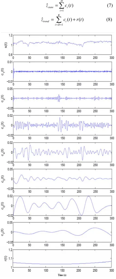
Figure 1 EEMD for HRV signal. From top to bottom are the HRV signal, c1(t)-c9(t), and r(t), respectively

In this contribution, the effect of the decomposition using the EEMD method is investigated with D=5, 6, 7. Fig.1 illustrates the decomposition of real HRV signal. The effects of the decomposition using the EEMD are that the added white noise series cancel each other in the final mean of the corresponding IMFs; the mean IMFs stay within the natural dyadic filter windows and thus significantly reduce the chance of mode mixing and preserve the dyadic property.

C. HRV Analysis

Time domain, frequency domain and nonlinear methods are employed for HRV analysis. The RR interval time series data is used for time domain analysis and nonlinear analysis, and the evenly re-sampled signal is used for frequency domain.

The time domain indices are: 1) SNDD, the standard deviation of the RR intervals; 2) RMMSD, the root mean square of the differences of successive RR intervals; 3) NN50, the number of consecutive RR intervals with absolute difference more than 50ms; 4) pNN50: the percentage value of NN50 with respect to all RR intervals. In the frequency domain analysis, the power spectrum density (PSD) estimation is calculated from the HRV signal with fast Fourier transform (FFT) based on Welch’s periodogram method. The commonly used frequency bands are very low frequency (VLF, 0~0.04Hz), low frequency (LF, 0.04~0.15Hz), and high frequency (HF, 0.15~0.4Hz). The frequency domain indices investigated here are: 1) VLF, absolute power of VLF band; 2) LF, absolute power of LF band; 3) HF, absolute power of HF band; 4) LF/HF, ratio between LF and HF band powers.

Figure 2 Power spectrum density of HRV signal

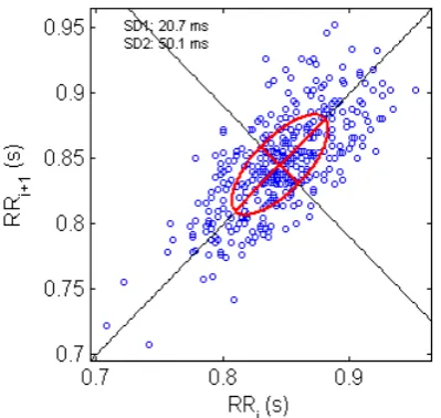
Poincaré plot is a commonly used nonlinear analysis method for HRV analysis. By plotting RRi+1 as a function of RRi, the graph could reveal the correlation between successive RR intervals (see Fig.2). An ellipse is fitted on the graph, and two indices could be derived: 1) SD1, the standard deviation of the points perpendicular to the line of symmetry; 2) SD2, the standard deviation of the points along the symmetry.

D. Validation

Figure 3 Poincaré plot analysis of RR intervals

providing a comparison of the effect between SPA and EEMD detrending methods.

In the generation of simulated HRV signals, four patterns of trends are considered as follows:

(1) The line pattern trend is denoted by

1( ) ₂

a a

trend t t

L

= − + ⋅ , 0≤ ≤t L (9)

where the parameter a =0.15 is chosen, and L is the duration of the trend.

(2) The Gaussian pattern trend is denoted by

2 ( / 2) 2( )

c t L

trend t = ⋅a e− − , 0≤ ≤t L (10)

where the parameters a=0.15, and c=5×10-4 are chosen. (3) The break pattern trend is denoted by

3

/ 2, 0 / 3

6

( ) ( / 3), / 3 2 / 3

/ 2, / 3 2 / 3

a t L

a

trend t a t L L t L

L

a L t L

≤ ≤

⎧ ⎪⎪

=⎨ − − < <

⎪

− ≤ ≤

⎪⎩

(11) where a=0.15 is chosen.

(4) The cosine pattern trend 4( ) cos(2 )

2 tr

a

trend t = πf t , 0≤ ≤t L (12)

where ftr=0.02 is chosen.

The process of generation of the artificial RR interval series mixed with trend is described as follows:

(1) An expression for the heart rate (HR) is firstly written as:

HR t( )=HR₀+A_lsin(2πf t_l )+A_hsin(2πf t_h ) (13)

where the parameters HR0=60bpm, Al=2, Ah=2.5, l

f =0.095Hz and f_h=0.275Hz are selected.

(2) The high frequency HRV signal is then formed by sampling

( ) 60 ( )

s

RR t trend

HR t

= + (14)

at a relative high frequency f_s =2000Hz such that

n s

n t

f

= where n=1, 2, ," N.

(3) The simulated RR interval series is unevenly re-sampled fromRR t( )in the way as follows: Record the

first data point pair, ( ,t RR t₁ ( ))₁ as the first time stamp

and RR interval pair ,

1 1

( ,t RR), Then proceed through each

sample, t_i, untilx_n ≥ −t_i t₁,; if x_n− ≤t_i x_n−1−t_i−1, (t₂, =t_i,

2 ( ))i

RR =RR t is selected as the second RR interval,

otherwise, ,

2 1 2 1

(t =ti−,RR =RR t(i−)) is selected. This is generated for the length of the simulated RR interval series is satisfied.

At the end of this process, a sequence

1 2

( , , , _n)

z= RR RR " RR , n=1, 2,"N₁

is get as a simulated RRI series with exactly known stationary and trend components.

Following [17], three metrics, SNR improvement (SNRimp) in decibel, mean squared error (MSE), and percent distortion (PRD) are used to quantify the detrending performance: 2 1 10 2 1 ( [ ] [ ]) 10 log ˆ ( [ ] [ ]) N stat n imp N stat stat n

z n z n SNR

z n z n = = − = −

∑

∑

2 1 1 ˆ ( [ ] [ ]) N stat stat n

MSE z n z n

N =

=

∑

2 1 2 1 ˆ ( [ ] [ ]) 100 [ ] N stat stat n N stat n

z n z n PDR z n = = − =

∑

∑

For a detrending method, the larger the SNRimp is, and the smaller the MSE and PRD are, a better performance of the detrending could be achieved.

In real HRV experiment, the ECG signals from MIT-BIH Fantasia database are used. 19 young and elderly subjects with 5 minutes’ segments of RRI series with normal beats only are derived for the experiment. The segments are derived without any beats overlapped. In the database, ECG signals were collected from healthy subjects undergoing 120 minutes of supine resting, and digitized at 250Hz, and R peaks were detected automatically and verified by visual inspection. In this way, 95 segments of RRI series are available both in the young and elderly group for the further experiment.

Statistical comparison between the indices of HRV signal calculated from young and elderly groups was performed by using independent t-test. All the data were expressed as mean±SD (standard deviation). The values of HRV indices were also compared between the two methods.

(a) (e) (i)

(b) (f) (j)

(c) (g) (k)

(d) (h) (l)

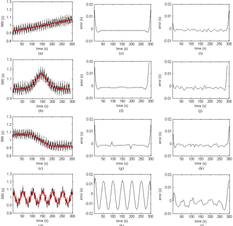
Figure 4 Trend filtering performance: (a)~(d) are simulated HRV signals with line, gauss, break, cosine pattern trend respectively; (e)~(h) are error traces corresponding to (a)~(d) using SPA method with λ=500 for detrending; (i)~(l) are error traces corresponding to (a)~(d) using EEMD method

with D=5 for detrending.

TABLE I.

COMPARING OF SPA AND EEMD METHODS FOR DETRENDING IN SIMULATED HRV SIGNALS

Line Gauss Break Cosine SNRimp

(db) （MSE s2_×

10-5_）

PRD

(%) SNR(db) imp （MSE s2_×

10-5_）

PRD

(%) SNR(db) imp （MSE s2_×

10-5_）

PRD

(%) SNR(db) imp （MSE s2_×

10-5_）

PRD (%)

SPA 23.3 0.89 0.3 25.8 1.03 0.32 26.4 1 0.32 14 11.16 1.06

Ⅲ. RESULTS AND DISCUSSION

The detrending performance in simulated RR interval series with trends using SPA method and EEMD method is shown in Fig. 3. Fig. 3 (a) ~ (d) shows simulated series with four patterns of trends: line, gauss, break, and cosine trends, respectively. The error trace, i.e. the difference between pure simulated series and detrended RRI is shown in Fig. 3 (e) ~ (h) using SPA method. The mean relative errors of them reduced after detrending, which show that the trends could influence the HRV analysis. Therefore, it is necessary to remove the trend before analysis. Fig 3 (i) ~ (l) shows error traces using EEMD method with D=5 for detrending. The EEMD method shows excellent performance for the line and gauss trends. Thus the EEMD method shows a better performance than the SPA method.

Table 1 further illustrates the performance of SPA method and EEMD method with D=5, 6, and 7 using three metrics: SNRimp, MSE, PRD. EEMD1, EEMD2, EEMD3 denotes the EEMD detrending method with D=5, 6, 7, respectively. In the case of cosine pattern trend, the EEMD method with D=6 shows obviously better performance. Table 1 shows that the EEMD method with

D=6 performs better than SPA method, especially when dealing with cosine pattern trend.

The comparison of trend extraction in real RR interval series by SPA method and EEMD method is illustrated in Fig. 4.

The HRV time domain, frequency domain, and poincaré plot indices derived from real RR interval series using SPA method and EEMD detrending method are presented in Table 2 and Table 3, respectively, to show the difference in young and elderly groups.

RR interval series are derived from R peaks in ECG. It should be noted that this unevenly spaced time series is unusual in that both axes of the signal are time intervals, and related to each other. The value of the signal at the current point is horizontal distance between the current and the previous adjacent point. This propriety hasn’t been emphasized in simulated HRV signals in [3, 9, 13]. However, we have paid much attention in this aspect of RR interval series, hoping to get more precise results for evaluating the detrending methods. Visual inspection in Fig. 3 reveals that both SPA and EEMD methods have satisfactorily removed the four pattern trends from the simulated RR interval series, and the error traces of the two methods illustrated that in line, gauss and break trend added HRV signals, the two methods acts generally comparable. However, in the case of cosine pattern trend, (a) (b)

Figure 4 Trend exaction performance: (a) is a real RR interval series and its trend extrated by SPA method withλ=500; and (b) is the same RR interval series and its trend extracted by EEMD method with D=6.

COMPARISON OF INDICES DERIVED FROM HRV SIGNALS OF YOUNG AND ELDERLY GROUPS DETRENDED BY EEMD METHOD.

Indices (unit)

indices young group

(n=95)

elderly group (n=95)

p value

SDNN (ms) SDNN 50.3±21.5 19.4±10.0 1.22×10-24

RMSSD (ms) RMSSD 57.0±30.6 23.3±12.4 1.87×10-17

NN50 NN50 84.7±57.8 11.3±18.1 3.55×10-21

pNN50 (%) pNN50 29.4±22.1 4.70±8.81 1.26×10-17

VLF (ms2

) VLF 22.1±32.3 4.91±7.61 1.92×10-6

LF (ms2_{) LF 1349±1295 192.3±305.6 1.63×10}-13

HF (ms2_{) HF 1381}

±1464 173.8±173.7 2.97×10-12

LF/HF LF/HF 1.86±2.68 1.36±1.33 0.11

SD1 (ms) SD1 40.3±21.7 16.5±8.73 1.87×10-17

SD2 (ms) SD2 57.9±23.5 21.6±11.8 6.07×10-27

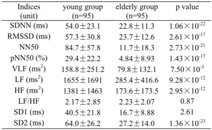
COMPARISON OF INDICES DERIVED FROM HRV SIGNALS OF YOUNG AND ELDERLY GROUPS DETRENDED BY SPA METHOD.

Indices

(unit) young group (n=95) elderly group (n=95) p value

SDNN (ms) 54.0±23.1 22.8±11.3 1.06×10-22

RMSSD (ms) 57.3±30.8 23.7±12.6 2.61×10-17

NN50 84.7±57.8 11.7±18.3 2.73×10-21

pNN50 (%) 29.4±22.2 4.84±8.93 1.43×10-17

VLF (ms2₎

158.8±251.2 79.8±132.1 7.50×10-3

LF (ms2_{) 1655±1691 285.4±416.6 9.28×10}-12

HF (ms2_{) 1381}

±1463 173.6±173.5 2.95×10-12

LF/HF 2.17±2.85 2.23±2.07 0.87

SD1 (ms) 40.5±21.8 16.7±8.88 2.61

the EEMD method with D=6 shows obviously better performance. Table 1 quantitatively shows that the EEMD method with D=6 is better than SPA method, especially when dealing with cosine pattern trend. This conclusion is again confirmed by real HRV signals in Fig. 4. The trend from 200s to 250s shown in Fig. 4 is more or less a cosine pattern, and the EEMD method gets a better trend exaction. As D=6 provides a compromise result in four situations in Table 1, this value is selected for further investigation when using EEMD method. Besides, the distortion of data end points could be observed for SPA method (see Fig. 1 (e) ~ (h)), and this problem can be relieved when using EEMD method [9].

Comparing the p value in Table 2 and Table 3, we can found that the HRV indices derived from RR interval series detrended by the EEMD method show more significant difference between the young and elderly groups, since a lower p value is received, indicating a better performance of EEMD method indirectly.

The numerical analysis for the performance of the EEMD detrending method for HRV analysis is presented using simulated HRV signals with trends, and compared with the SPA method. However, a theoretical study is still desired to be explored. The detrending method is used in HRV analysis related to age. Results show that most of the HRV indices derived from the HRV signals detrended by the EEMD method can improve the ability for distinguishing between young and elderly groups except the index HF. For our future work, we shall conduct more experiments to evaluate the influence of the EEMD detrending method in HRV indices, especially in terms of HF.

Ⅳ. CONCLUSION

In this paper, comparison results of the EEMD and SPA detrending methods show that the EEMD is superior to SPA in detrending RR interval series. The main advantage of the EEMD method, compared to SPA method is that EEMD can partly relieve the adverse end point effect, and more importantly, EEMD method shows an excellent performance in extraction of cosine pattern trends. The conclusion is not restricted to HRV analysis only, but can also be applied to other physiological signals, such as blood pressure variability and detrending of EEG signals in EEG analysis.

ACKNOWLEDGMENT

This work was supported by the National Natural Science Foundation of China (No.21105127), and the Science Foundation of Hunan Province, China (No. 12JJ6061).

REFERENCES

[1] Task Force of the European Society of Cardiology the North American Society of Pacing Electrophysiology. Heart Rate Variability: Standards of Measurement, Physiological Interpretation, and Clinical Use. Circulation, 1996, 93(5):1043-1065.

[2] Li H, Kwong S, Yang L, Huang D, Xiao D. Hilbert-Huang transform for analysis of heart rate variability in cardiac health. IEEE/ACM Trans Comput Biol Bioinform. 2011, 8(6):1557- 167.

[3] Yoo C S, YI S H. Effects of detrending for analysis of heart rate variability and applications to the estimation of depth of anesthesia. Journal of the Korean Physical Society, 2004, 44(3):561-568.

[4] Tarvainen M P, Niskanen J P. Kubios HRV User's Guide.[2013-5-8].

http://kubios.uef.fi/media/Kubios_HRV_2.1_Users_Guide. pdf.

[5] Wen Feng, HE Fang-tian. An efficient method of addressing ectopic beats: new insight into data preprocessing of heart rate variability analysis. Journal of Zhejiang University-SCIENCE B (Biomedicine & Biotechnology), 2011,12(12): 976-982.

[6] Tarvainen M P, Ranta-aho P O, Karjalainen P A. An Advanced Detrending Method With Application to HRV Analysis. IEEE TRANSACTIONS ON BIOMEDICAL ENGINEERING, 2002,49(2):172-175.

[7] Litvack D A, Oberlander T F, Carney L H, Saul J P. Time and frequency domain methods for heart rate variability analysis: a methodological comparison. Psychophysiology, 1995, 32(5):492-504.

[8] Mitov I P. A method for assessment and processing of biomedical signals containing trend and periodic components. Medical Engineering & Physics, 1998, 20(9), 660~668.

[9] Shafqat K, Pal S K, Kyriacou P A. Evaluation of two detrending techniques for application in Heart Rate Variability// 29th Annual International Conference of the IEEE Engineering in Medicine and Biology Society. IEEE: Lyon, 2007: 22-26.

[10]Eleuteri A, Fisher A C, Groves D, Dewhurst C J. An Efficient Time-Varying Filter for Detrending and Bandwidth Limiting the Heart Rate Variability Tachogram without Resampling: MATLAB Open-Source Code and Internet Web-Based Implementation. [2013-5-8]. http://www.hindawi.com/journals/cmmm/2012/578785/. [11]Huang N E, Shen Z, Long S R, Wu M C, Shih H H, Zheng

Q, Yen N C, Tung C C, Liu H. The empirical mode decomposition and the Hilbert spectrum for nonlinear and non-stationary time series analysis. Proc. R. Soc. Lond. A, 1998, 454(1971):903-995.

[12]Kabir M A, Shahnaz C. Denoising of ECG signals based on noise reduction algorithms in EMD and wavelet domains. Biomedical Signal Processing and Control, 2012, 7(5):481-489.

[13]Li Liping, Li Ke, Liu Changchun, Liu Chengyu. Comparison of Detrending Methods in Spectral Analysis of Heart Rate Variability. Research Journal of Applied Sciences, Engineering and Technology, 2011,3(9): 1014-1021.

[14]Wu Z, Huang, N E. Ensemble empirical mode decomposition: a noise-assisted data analysis method. Advances in Adaptive Data Analysis. 2009, 1(1):1-41. [15]Torres M E, Colominas M A, Schlotthauer G, Flandrin P.

A complete ensemble empirical mode decomposition with adaptive noise. // 2011 IEEE International Conference on Speech and Signal Processing. IEEE:Acoustics, 2011:22-27.

[17]Chang K M, Liu S H. Gaussian Noise Filtering from ECG by Wiener Filter and Ensemble Empirical Mode Decomposition. J Sign Process Syst 2011, 64:249-264. [18]Clifford G D. Signal Processing Methods for Heart Rate

Variability. Oxford: Oxford University, 2002.

[19]Abhishekh A H, Nisarga P, Kisan R, Meghana A, Chandran S, Raju T, Sathyaprabha T N. Influence of age and gender on autonomic regulation of heart. J Clin Monit Comput, 2013, 27(3):259-264.

[20]Voss A, Heitmann A, Schroeder R, Peters A, Perz S. Short-term heart rate variability-age dependence in healthy subjects. PHYSIOLOGICAL MEASUREMENT, 2012,33(8):1289-311..

Chao Zeng was born in Yiyang, China in August, 1982. He

received his B.S. from Xiangtan University in 2005. He is now a Ph.D. candidate in Central South University, Changsha, China. He is also a lecture in Shihezi University, Shihezi, China since 2010. His major field of study covers biomedical image and biomedical signal processing techniques.

Xiaowen Xu was born in Jiangsu, China in May, 1978. He