A weakly nonlinear model for multi-modal evolution of wind-generated long internal waves in a closed basin

www.nonlin-processes-geophys.net/16/487/2009/ © Author(s) 2009. This work is distributed under the Creative Commons Attribution 3.0 License.

Nonlinear Processes

in Geophysics

A weakly nonlinear model for multi-modal evolution of

wind-generated long internal waves in a closed basin

T. Sakai and L. G. Redekopp

Department of Aerospace & Mechanical Engineering, University of Southern California, Los Angeles, CA 90089-1191, USA Received: 17 February 2009 – Revised: 1 July 2009 – Accepted: 2 July 2009 – Published: 17 July 2009

Abstract. A weakly nonlinear evolution model that accounts for multi-modal interaction in a small, continuously stratified lake of variable depth is derived. In particular, an evolution model for the first two vertical modes in a lake that is sub-ject to wind stress forcing is numerically simulated. Defining modal energies, energy transfer between the first and the sec-ond vertical modes is calculated for several different forms of the density stratification. Modal energy transfer mainly occurs during reflection of mode-one waves at the vertical end walls, and it is shown that the amount of energy trans-fer from the first to the second mode is greatly dependent on the shape of the stratification profile. Also, the initial modal energy partition at the wind setup is shown to depend signif-icantly on the penetration depth of the internal shear stress induced by the wind stress, especially if the stress distribu-tion extends into the upper levels of the metalimnion.

1 Introduction

Thermally stratified lakes are often subject to wind stress forcing, generating basin scale internal waves that are the primary energy source for driving material transport in lakes. For modeling of such long internal waves in lakes, a simple two-layer stratification model has been preferably used since its establishment in early 20th century. The model is a rea-sonable approximation as long as the lake is strongly strat-ified (e.g., during summer) and the density stratification is confined to a thin layer between a homogeneous epilimnion (upper warm, mixed layer) and a homogeneous hypolimnion (lower cold, stagnant layer). The stratification is generally continuous, and its structure varies seasonally, with conse-quent seasonal effects on the evolution of internal waves

(An-Correspondence to: T. Sakai

([email protected])

tenucci et al., 2000). In a continuously stratified fluid, as is well-known from linear analysis, the vertical distribution of fluid velocities and displacement of isopyicnal surfaces pos-sess multi-modal structures. The two-layer model accounts only for the first baroclinic mode, and it implicitly neglects all the other baroclinic modes in the field.

h

b

x = 0 x = L

z = 0

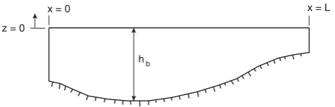
Fig. 1. Basin configuration.

an isolated phenomenon in lakes, but has also been reported in oceanography (e.g., Bogucki et al., 2005; Gerkema, 2003). It is routine to solve the vertical normal mode equation for a given stratification profile to obtain eigenfrequencies and eigenfunctions for particular modes of interest. However, such normal mode equations are based on linear theory, and the solutions therefore are linearly independent, yielding no information about modal interactions. Gerkema (2001, 2003) adopted a multi-modal approach, and formulated a weakly-non1inear and weakly-dispersive multi-modal evolution sys-tem that was successfully applied to the oceanography prob-lem. Utilizing a stratification profile in the Bay of Biscay in which the third vertical mode is dominant, he demonstrated that energy may leak (not dissipation) from the third mode to lower modes. Also, the amount of energy leakage was shown to be highly dependent on the strength of the stratifi-cation. H¨uttemann and Hutter (2001) observed emergence of solitary waves of the second vertical mode when a mode-one soliton ran over a sill in a long laboratory channel. At the same time, Vlasenko and Hutter (2001) simulated the two-dimensional Navier–Stokes equations in the same configu-ration as H¨uttemann’s experiment, and detailed structure of the flow field was obtained, confirming that both the first and the second mode solitons are very close to those obtained by Korteweg–de Vries (KdV) theory.

To understand the full basin energetics in lakes, it is essen-tial to determine the modal energy distribution among domi-nant vertical modes in a system allowing full bi-directional propagation of the linearly independent modes. Nonlin-ear models are the essential for capturing inter-mode en-ergy transfer. In this paper, we derive a weakly-nonlinear, wind-forced evolution model by applying the multi-modal approach that yields an evolution equation for each vertical mode with inter-modal interactions through nonlinear terms. For fundamental study, we limit the vertical modes in the model to the first two modes which are energetically domi-nant in many cases. The model is numerically solved, and we study the modal energetics for various parameters of the modeled stratification and the wind forcing.

2 Derivation of a nonlinear, multi-modal system

We consider a closed basin containing continuously stratified fluid. To isolate the physics from the effect of the earth’s

rota-tion, we neglect Coriolis acceleration of fluid elements. As-suming width of the lake is sufficiently narrow and uniform, we start with the two-dimensional, incompressible, Boussi-nesq approximated, inviscid equations of motion that are per-turbed from the basic state of hydrostatic equilibrium:

ux+wz=0,

ut +uux+wuz= −px+τz, wt+uwx+wwz= −pz−σ, σt+uσx+wσz=N2w.

(1)

In these equations, subscripts denote partial derivatives,p is the density normalized pressure,τ is the density normal-ized horizontal stress to account for wind forcing and bottom friction along the horizontal (x) axis,σis the perturbed buoy-ancy (σ=ρg/ρ0), andN is buoyancy frequency defined by

using a reference densityρ0, static densityρs(z)and gravity

gas

N2(z)= − g

ρ0

dρs(z)

dz . (2)

We assume the field domain that is enclosed by a non-deformable upper surface, vertical end walls and nonuniform (variable depth) bottom surface (Fig. 1).

Solutions of Eq. (1) are dictated by slip-free, impermeable and non-deformable boundary conditions:

w=0 atz=0, w= −udhb

dx atz= −hb, u=0 atx=0 andx=L.

(3)

The length of the lake is denoted byL, andhbis the vari-able depth of the fluid. We introduce a long wave scaling to horizontal space and time coordinates, and also define a slow space coordinateξ,

(X, T )=µ(x, t ), ξ =µ3x, (4) whereµ∼h/ l1 is the long wave scaling parameter with ha depth scale (e.g., thickness of surface mixed layer) and l is typical (long) wave length scale. We assume that the topography varies slowly in space (i.e.,hbis a function ofξ only) so that topographic interaction terms will appear in the second-order approximation. We then expand the dependent variables in an asymptotic series of the form

(u, p, σ )=(u(1), p(1), σ(1))+2(u(2),· · ·)+ · · ·, w=µ(w(1)+w(2)+ · · ·),

τ =µ2(τ(1)+τ(2)+ · · ·),

(5)

amplitude parameter so that wind forcing or benthic fric-tional dissipation appears first in the second order balance (i.e., weak forcing and weak damping), as do the leading ef-fects of variable depth. We introduce the familiar KdV scal-ing (i.e.,=µ2), in order to balance weak nonlinearity and leading-order non-hydrostatic correction at the same level of approximation.

Transforming independent variables using Eq. (4), and substituting Eq. (5) into Eq. (1), the leading-order balance gives the linear equation set

u(_X1)+wz(1)=0, u(_T1)+p(_X1)=0, pz(1)+σ(1)=0, σ_T(1)−N2w(1) =0.

(6)

From Eq. (6) one can obtain a single equation in favor of w(1):

w(_{zzT T}1) +N2w(_XX1) =0. (7) One can seek, in the sense of a consistent asymptotic ap-proximation, a slowly-varying normal mode solution in the form

w(1)=W (X, ξ, T )φ (ξ, z), (8) whereφ=0 atz=0 (upper surface) andz=−hb(bottom sur-face) to satisfy leading order boundary conditions. The de-pendence of the eigenfunction on the slow longitudinal coor-dinateξ arises from the inhomogeneity of the wave guide in the propagation direction (i.e., variable depthh(ξ )). We note that the analysis can be readily extended to include a slowly-varying wave guide width, as in the single-mode model pre-sented in our unpublished report, but we choose to not in-clude that further complication in the present study. Sub-stituting Eq. (8) into Eq. (7) one can construct a standard boundary value problem along the vertical line for everyξ:

φ_n00+N

2_(z)

c2

n(ξ )

φn=0; φn|z=0=φn|z=−hb =0;

n=1,2,· · ·,

(9)

wherecnis an eigenvalue,φnis the corresponding eigenfunc-tion, and primes denote partial derivatives with respect toz. The corresponding orthogonality relation is

Z 0

−hb

φ_m0 φ_n0dz= In

c2

n δmn;

Z 0

−hb

N2φmφndz=Inδmn;

andIn= Z 0

−hb

N2φ_n2dz,

(10)

whereδmnis Kroneker’s delta.

All dependent variables are now expanded using the con-sistency implied by Eq. (6):

u(1)=X

n

U_n(1)(X, ξ, T )φ_n0(ξ, z),

w(1) =X

n

W_n(1)(X, ξ, T )φn(ξ, z),

p(1)=X

n

P_n(1)(X, ξ, T )φ_n0(ξ, z),

σ(1)=X

n

Z(_n1)(X, ξ, T )N2(z)φn(ξ, z).

(11)

Substituting Eq. (11) into Eq. (6), employing Eq. (10), and eliminatingWn(1)andPn(1), we obtain the coupled pair of evo-lution equations

U_nT(1)+c_n2Z_nX(1)=0, Z_nT(1)+U_nX(1) =0.

(12)

As evident in Eq. (11)Znis the modal isopycnal amplitude andUn is the modal amplitude for the horizontal velocity. Eq. (12) defines a set of independent, linear, bi-directional waves propagating with their respective eigenspeedscn.

Proceeding to the next order balance using Eq. (5) leads to the inhomogeneous set

u_X(2)+wz(2)= −u(ξ1),

u_T(2)+p_X(2)= −{u(1)u_X(1)+w(1)uz(1)} +τz(1), pz(2)+σ(2)= −w_T(1),

σ_T(2)−N2w(2)= −{(u(1)σ(1))X+(w(1)σ(1))z}.

(13)

Note that the leading-order stress term τ(1) appears and that the boundary condition in the vertical direction gives

w(2) =0 atz=0,

w(2) = −u(1)dhb

dξ atz= −hb.

(14)

The term u(_ξ1) in the first equation in Eq. (13) is the leading-order effect of slowly varying depth; the brack-eted terms in the second equation (x-momentum) contain the leading-order nonlinear acceleration; the term w(_T1) in the third equation (z-momentum) is the leading-order non-hydrostatic correction; and the bracketed terms in the last equation (continuity) define the leading-order buoyancy flux correction.

first equation in Eq. 13), multiplying byφ_n0, then integrating over the physicalzdomain and using Eq. (10), one obtains

In c2

n U_nX(2)+

Z 0

−hb

φ0_nw(_z2)dz= −In

c2

n U_nξ(1)

−X

i U_i(1)

Z 0

−hb

φ_n0∂φ 0 i

∂ξ dz. (15)

Using Eq. (14), the integral term on the left side of Eq. (15) can be evaluated via integration by parts

Z 0

−hb

φ0_nw_z(2)dz=X

i

[φ_n0φ0_i]_z=−h

b

dhb dξ U

(1) i

−

Z 0

−hb

φ_n00w(2)dz, (16)

and w(2) can be eliminated by using the last equation in Eq. (13). Through this procedure Eq. (15) yields an evolu-tion equaevolu-tion for the isopycnal amplitude funcevolu-tionZn. The evolution equation forUncan be obtained by substituting the expansions into momentum equations in Eq. (13) and using Eq. (10). After some algebraic manipulation, the evolution of the leading-order field variables is obtained in the form:

U_nT(2)+c2_nZ_nX(2)=X

ij n

a_nij(u)U_i(1)U_{j X}(1)+b_nij(u)U_iX(1)U_j(1)o

+X

i

dniU_iXXT(1)

− ∂c

2

n ∂ξ Z

(1) n −c2nZ

(1) nξ −

X i

φ_n0∂φ

0 i ∂ξ

c_i2Z(_i1)

+ksnτs(1)−kbnτ_b(1)+ 1 c2

n D

N2φnτ(1) E

(17)

and

Z_nT(2)+U_nX(2)= −X

ij n

a_nij(σ )(U_i(1)Z_j(1))X+b(σ )nijU (1) iXZ

(1) j

o

−U_nξ(1)

−X

i (

c2_n In[φ

0

nφi]z=−hb

dhb dξ +

φ0_nφ

0 i ∂ξ

)

U_i(1). (18)

We point out that the first-order stress τ(1) has been di-vided into two parts: τs(1)is the wind stress at the lake sur-face, and τ_b(1) is the bottom shear stress. The coefficients

appearing in Eqs. (17, 18) are defined by the following set of relations:

a(u)_nij =Dφ_n0φ_i0φ0_jE, b(u)_nij =

* N2

c2_j φ 0 nφiφj

+ ,

a(σ )_nij =

* N2

c2

n φnφi0φj

+

, b(σ )_nij =

* N2

c2

n φ_n0φiφj

+ ,

dnj =φnφj, ksn= c2_n In

φ_n0|_z=0, kbn= c2_n In

φ0_n|_z=−h

b,

where h· · ·i ≡ c

2

n In

Z 0

−hb

(· · ·)dz.

(19)

The termU_iX(1)Z(_j1) appearing in Eq. (18) (i.e., continuity equation) derives from the vertical buoyancy flux term, and one observes that the equation cannot be integrated with re-spect toXbecause of the presence of this term. Hence the velocity and isopycnal amplitudes can not be decoupled into a single, second-order-in-time wave equation. Combining Eq. (12) and Eqs. (17, 18), and transforming the indepen-dent variables back to their non-scaled form, we obtain the weakly-nonlinear evolution equation set:

Unt+(c2_nZn)x= −X

ij n

a_nij(u)UiUj x+b(u)_nijUixUjo

+X

i

dniUixxt− X

i

rnici2Zi

+ksnτs −kbnτb+ 1 c2

n D

N2φnτ E

(20) and

Znt +Unx = −X

ij n

a_nij(σ )(UiZj)x+b(σ )_nijUixZjo

−X

i

sniUi, (21)

where rni=

φ_n0∂φ

0 i ∂x

;sni= c_n2 In

[φ_n0φ_i0]_z=−hb

dhb

dx +rni. (22) The rni coefficient, containing effects of variable depth (alt., spatially varying eigenvalue), can be further evaluated by using Eq. (9) and Eq. (10). The final expression is given here without derivation:

rni=         

(cn/ci)2 1−(ci/cn)2

_φ0 n φ_i0

z=−hb

Ii In

d lnc2_i

dx , ifi6=n, 1

2 d dx ln

In c4

n

, ifi=n.

(23)

that the hydrostatic representation of the modal structure is no longer valid at second order. The linear terms scaled by the coefficientsrij andsij appearing on the right hand side of the equations capture the effect of self-modal distortion and cross-modal transfer resulting from variable depth ef-fects. That these terms appear at this order is a direct con-sequence of the slowly-varying depth assumption, which in turn is required in order to derive a rationally-based evolution system where the underlying dynamics is represented by the linear modes of the system. A more general derivation of the topographic coupling terms for uni-directional wave propa-gation over topographies that vary both along and transverse to the propagation direction has been developed by Griffiths and Grimshaw (2007) in their study of internal tide at conti-nental shelf regions.

The wind stressτs can be expressed in terms of a friction velocityu∗0and a prescribed, dimensionless stress

distribu-tion funcdistribu-tionF (x, t ).

τs =u2∗0F (x, t ). (24)

The vertical distribution of the horizontal stress induced by the wind, varying from its surface valueτs, is also needed to determine the coefficienthN2φnτiin Eq. (20). Assuming only the wind stress contributes to the integral, we modelτ using a static, vertical stress distribution functionτ (z)˜

τ =u2_∗0F (x, t )τ (z)˜ =τsτ (z),˜ (25) whereτ˜is dimensionless, andτ (˜ 0)=1. The bottom stressτb can be modeled assuming that the boundary layer is turbulent and using a friction coefficientCf:

τb=Cfub|ub|

=Cf X

i

Ui(x, t )φi0|z=−hb

X j

Uj(x, t )φj0|z=−hb

. (26)

The value ofCf for shallow water flows is typically quite small, of order 10−3(cf., Baines, 1995), with recommended value Cf=0.0025 for weakly nonlinear long wave theory (Grimshaw, 2002). We fixedCf at this value throughout this study, and the value ofubin Eq. (26) is the inviscid, wave-induced velocity at the bottom surface. We take the contri-bution of bottom friction to a particular mode in the form

τb≡τbn=CfUnφ_n0|_z=−h

b

X j

Ujφ_j0|_z=−h

b

. (27)

3 The two-mode evolution model

In this study we limit the number of active vertical modes to the lowest two (V1: mode-one; V2: mode-two). This re-striction is made in order to reduce the complexity of the evolution model while retaining the energetically-dominant

modes in the system. To reduce the number of free parame-ters in the evolution equation, we introduce non-dimensional variables by use of the following scales: x byL; Zn andz by the surface mixing layer thicknessh1;tby 2L/c0, where

c0is a reference phase speed taken as a spatial average of V1

phase speed;cn(orc0) byN0h1, whereN0is the maximum

buoyancy frequency; andUn byN0h2₁. After recasting the

Eqs. (20, 21) in a dimensionless form, we have an evolution equation set for V1 in the form:

Ut + 2 c0

(c₁2Y )x= 2 c0

{µ111U Ux+µ112U Vx

+µ121V Ux+µ122V Vx} +S2{d11Uxxt+d12Vxxt}

− 2

c0

{κ11Y +κ12Z} +

2c0

W

˜

ks1F (x, t )

− 2

c0S

kb1CfU|U φ10 +V φ

0

2|z=−hb (28)

and Yt +

2 c0

Ux= 2 c0

{−σ111(U Y )x−σ112(U Z)x

−σ121(V Y )x−σ122(V Z)x

+ν111Y Ux+ν112Y Vx+ν121ZUx+ν122ZVx}

− 2

c0

{λ11U+λ12V}, (29)

and corresponding set for V2 in the form:

Vt + 2 c0

(c2₂Z)x = 2 c0

{µ211U Ux+µ212U Vx

+µ221V Ux+µ222V Vx} +S2{d21Uxxt+d22Vxxt}

− 2

c0

{κ21Y +κ22Z} +

2c0

W

˜

ks2F (x, t )

− 2

c0S

kb2CfV|U φ10 +V φ

0

2|z=−hb (30)

and Zt +

2 c0

Vx= 2 c0

{−σ211(U Y )x−σ212(U Z)x

−σ221(V Y )x−σ222(V Z)x

+ν211Y Ux+ν212Y Vx+ν221ZUx+ν222ZVx}

− 2

c0

{λ21U+λ22V}. (31)

0 1 −5

−4 −3 −2 −1 0

N2

z

h ₂=0.5 h ₂=1 h ₂=2

0 1

φ

1

−1 0 1

φ₂

0 1

−5 −4 −3 −2 −1 0

z

N _h2=0 N_h2=0.1

N_h2=0.5

0 1 −1 0 1

0 1

−5 −4 −3 −2 −1 0

z

h₃=1 h₃=2 h₃=3

0 1 −1 0 1

(a)

(b)

(c)

N2 φ₁ φ₂

N2 φ₁ φ₂

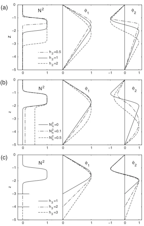
Fig. 2. Profile of buoyancy frequencyN2, vertical mode-1 eigen-functionφ1and vertical mode-2 eigenfunctionφ2for different (a) metalimnion thicknessh2, (b) hypolimnion stratificationN_h2, and

(c) hypolimnion thicknessh3.

The shallow water parameterS, defined asS=h1/L, enters

as a quadratic scaling factor in the dispersive terms appear-ing in Eq. (28) and Eq. (30), and as an inverse scalappear-ing factor multiplying the bottom friction terms in the same equations. Also appearing in Eq. (28) and Eq. (30) is the Wedderburn numberW. This parameter is inversely proportional to the magnitude of the wind stress (cf., Imberger and Patterson, 1990 and Horn et al., 2001), is defined by the relation W = c

2 0/L

u2_∗0/ h1

= c

2 0h1

u2_∗0L. (32)

The Wedderburn number measures the baroclinic pressure gradient relative to the vertical gradient of the imposed wind stress represented in terms of the water friction velocityu∗0.

Using measured values of the drag coefficient induced by wind blowing over a wavy free surface, as summarized by Phillips (1966), typical values of the Wedderburn number can

be roughly estimated by the relation W≈105SU₁₀−2, where U10is the wind speed in ms−1measured at an elevation of

10 m above the mean water surface. Data from both labora-tory experiments and field measurements reveal that signif-icant internal wave dynamics are observed when the Wed-derburn number lies in the range 1<W <5 (cf., Horn et al., 2001). The quantityk˜snin Eq. (28) and Eq. (30) is the modi-fied wind forcing factor defined as

˜

ksn=ksn+ 1 c2

n

hN2φnτ (z)˜ i. (33) With this evolution model in hand, we set up the ver-tical structure which qualitatively represents typical strati-fication profiles in lakes. We adopt a three-layer, contin-uously varying density structure comprising a well-mixed layer (epilimnion) of thicknessh1, a thermoclinic layer

(met-alimnion) of thickness h2having uniform density gradient,

and a weakly-stratified deep water (hypolimnion) of thick-ness h3. The square of the corresponding buoyancy

fre-quency is expressed by a simple formula in a dimensionless form:

N2(z)= 1

2

1−tanh _z+1

δ

+(1−N_h2)

tanh

_z+1+h

2

δ

−1

, (34)

whereδ is a smoothing parameter across the interface be-tween the metalimnion and either the epilimnion or hy-polimnion, and N_h2 is the buoyancy frequency in the hy-polimnion relative to the value in the metalimnion.

We present in Fig. 2 selected profiles ofN2(z)for different h2,N_h2andh3, and their corresponding eigenfunctions of V1

(φ1) and V2 (φ2).

The eigenfunctions are normalized by their maximum values. If there is no stratification in the hypolimnion (Fig. 2a, c),φ1 attains the maximum value within the

met-alimnion, and φ2 has extremal values near the top and the

bottom portions of the metalimnion, implying that isopycnal displacements of V1 and V2 are both pronounced in the met-alimnion, which is stretched and squeezed by V2. A slight increase in the stratification of the hypolimnion leaves the shape ofφ1nearly unchanged, butφ2is significantly altered

having its maximum value shifted downward into the hy-polimnion (Fig. 2b). Stratification in the hyhy-polimnion en-hances vertical displacements in the hypolimnion via V2, and also enhances the horizontal motions at the lake bottom where the gradient ofφ2is maximum. It is evident, therefore,

that weak stratification in the hypolimnion can significantly enhance benthic stimulation from wind-forced V2 internal waves.

Table 1. Coefficients of selected nonlinear terms for different metalimnion thicknessh2. The thickness and the stratification of the hypolimnion are fixed ash3=3 andNh2=0, respectively. The

smoothing parameter is chosen asδ=0.1 forh2=1 and 2,δ=0.05 forh2=0.5, andδ=0.025 forh2=0.25.

h2 0.25 0.5 1 2

µ111 0.943 0.792 0.554 0.222

σ111 −0.314 −0.264 −0.185 −0.074

ν111 0.314 0.264 0.185 0.074

µ122 12.166 6.460 3.329 1.234

σ122 −0.089 −0.087 −0.078 −0.049

ν122 0.175 0.169 0.148 0.090

µ222 14.834 7.169 3.312 1.383

σ₂₂₂ −4.945 −2.390 −1.104 −0.461

ν222 4.945 2.390 1.104 0.461

µ211 0.413 0.336 0.237 0.130

σ211 0.467 0.426 0.373 0.331

ν211 15.195 7.200 3.345 1.522

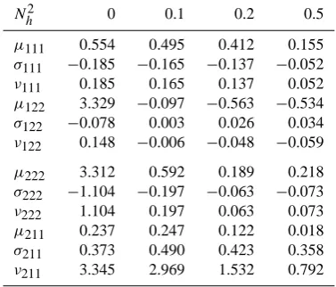
Table 2. Coefficients of selected nonlinear terms for different

strati-ficationN_h2in the hypolimnion. The thicknesses of the metalimnion and the hypolimnion are fixed ash2=1 andh3=1, respectively. The smoothing parameter is fixed asδ=0.1.

N_h2 0 0.1 0.2 0.5

µ111 0.554 0.495 0.412 0.155

σ111 −0.185 −0.165 −0.137 −0.052

ν111 0.185 0.165 0.137 0.052

µ122 3.329 −0.097 −0.563 −0.534

σ₁₂₂ −0.078 0.003 0.026 0.034

ν122 0.148 −0.006 −0.048 −0.059

µ222 3.312 0.592 0.189 0.218

σ222 −1.104 −0.197 −0.063 −0.073

ν222 1.104 0.197 0.063 0.073

µ211 0.237 0.247 0.122 0.018

σ211 0.373 0.490 0.423 0.358

ν211 3.345 2.969 1.532 0.792

numerical integration for several different values ofh2

(Ta-ble 1),N_h2(Table 2) andh3(Table 3), where we provide only

coefficients of self-nonlinear (µ111,µ222,· · ·) and

coupling-nonlinear terms (µ122,µ211,· · ·) for the sake of later

discus-sions.

The most notable result is the sensitivity of the coefficients with respect to the thickness of the metalimnion (see Ta-ble 1). Some of the coefficients (µ222,ν211,µ122) become

very large as the metalimnion thickness decreases. Self-nonlinear coefficients of V2 are larger than their V1 counter-parts by roughly an order of magnitude. This is due to the fact that the gradient ofφ2in the middle of the metalimnion

be-Table 3. Coefficients of selected nonlinear terms for different

hy-polimnion thicknessh3. The thickness of the metalimnion, the strat-ification of the hypolimnion and the smoothing paramter are fixed ash2=1,N_h2=0 andδ=0.1.

h3 1 2 3 4

µ111 0.000 0.389 0.554 0.642

σ111 0.000 −0.130 −0.185 −0.214

ν111 0.000 0.130 0.185 0.214

µ122 0.000 2.195 3.329 4.048

σ122 0.000 −0.058 −0.078 −0.088

ν122 0.000 0.109 0.148 0.168

µ222 3.113 3.275 3.312 3.325

σ222 −1.038 −1.092 −1.104 −1.108

ν222 1.038 1.092 1.104 1.108

µ211 0.271 0.254 0.237 0.225

σ211 0.548 0.429 0.373 0.341

ν211 3.248 3.345 3.345 3.328

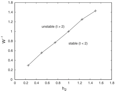
comes larger for thinner metalimnion (see Fig. 2a). Depend-ing on the wave amplitudes, the appearance of these large co-efficients can cause the corresponding nonlinear terms to be larger than linear terms. The asymptotic assumption that was used to derive the evolution model then becomes disordered, necessitating that the model be restricted to wind-forcings that yield smaller amplitudes. In fact, when the evolution model was simulated (numerical method and run configura-tion are briefly described in Sect. 4), numerical instability was encountered as the strength of the wind stress forcing was increased. In Fig. 3, for example, the threshold Wedder-burn number for achieving stable numerical integration up to two V1 seiche periods as a function of the metalimnion thickness for a fixed total depth is plotted.

For thinner metalimnion, our numerical code is not capa-ble of performing long-time integration for strong wind forc-ing. We also found during numerical testing that the insta-bility is pronounced for higher numerical resolution. When all the nonlinear coupling terms between the two modes are turned off, numerical integration becomes stable even for strong wind forcing. The precise mechanism of how the instability is triggered is not straight forward. We conjec-ture that the large nonlinear coefficients enhance excessive energy transfer between V1 and V2 (i.e., widely disparate length scales), and also generate excessive energy levels at high wave numbers.

Based on the data presented by Horn et al. (2001), show-ing that the regime of active, wind-driven, V1 nonlinear in-ternal wave motion occurs when 0.2<W−1<1, and the rep-resentation of the Wedderburn number in terms of the shal-low water parameterSand the 10 m wind speedU10given in

0 0.2 0.4 0.6 0.8 1 1.2 1.4 1.6 1.8 0

0.2 0.4 0.6 0.8 1 1.2 1.4 1.8

h₂

W

−1

stable (t < 2) unstable (t > 2)

Fig. 3. Model stability limit in inverse Wedderburn numberW−1

as a function of the metalimnion thicknessh2for a fixed total depth (h1+h2+h3=5); (hs=1.0).

N

2

(z)

h

1

h

2

h

s

τ

s

τ

(z)

Fig. 4. Penetration of the wind stress into the metalimnion.

wave dynamics provided the metalimnion is not too thin (i.e., h2≥0.8, say).

Adding stratification to the hypolimnion decreases the magnitude of the nonlinear coupling coefficients (see Ta-ble 2), making the model less nonlinear and, hence, allow-ing larger wind energy input to the system. Reducallow-ing the thickness of the hypolimnion decreases the magnitude of V1 nonlinear coefficients, while V2 counterparts change only slightly. It is well known from KdV theory that the weak self-nonlinearity is identically zero for a completely symmet-ric vertical structure. This is realized in Table 3 forh3=1

(h1=h2=1), albeit values of the cross nonlinear terms (µ112,

µ121,· · ·), which are not included in the table, are non-zero

for this configuration.

4 Wind forced response of two-mode model

When the wind stress is applied over the lake surface, a hor-izontal shear stress progressively penetrates across the epil-imnion. Heaps and Ramsbottom (1966) found an analytical solution for the shear stress distribution by solving the two-dimensional, linear hydrostatic equations. In this case, the wind induced shear stress decreases to zero linearly across the epilimnion. For a continuously stratified field, however, the shear stress distribution is not well known. The most commonly assumed form takes the shear stress diminishing linearly to a zero value at the base of the epilimnion, and the stress is zero beyond (e.g., see Monismith, 1987). With this assumption, the stress termhN2φnτ˜iin the wind stress factor

˜

ksis identically zero. In this study, we adopt the linear stress function, but allow the stress to penetrate the metalimnion (see Fig. 4).

The stress function is expressed by introducing a stress penetration depthhs as a parameter:

˜

τ (z)=

    

z+hs hs

, if −hs < z≤0, 0, otherwise.

(35)

Furthermore, in this study the wind stress functionF (x, t ) is uniform over the surface of the lake and, is switched on and off in time. Lake response to variations in the spatio-temporal character of the wind forcing was studied in some detail in the uni-modal study by authors (unpublished report). Equations (28–31) are solved numerically using the 4th-order compact finite difference scheme (Lele, 1992) for spa-tial discretization, and a forward-in-time 3rd-order Adams– Bashforth scheme. The 4th-order compact filter (Lele, 1992; Slinn and Riley, 1998) is applied every 10 time steps for dealiasing and stabilization. Numerical resolution that fol-low was chosen using 1025 points for spatial domain and a time step1t=5×10−5. This high resolution configuration, in conjunction with the spatial descretization scheme with “spectral-like” resolution, sufficiently resolves steep nonlin-ear fronts and oscillatory waves.

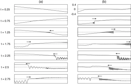
Figure 5 shows the evolution of isopycnal amplitudes (Y andZ) at several selected times following the initiation of a wind event in a lake of uniform depth withh2=1,h3=3.

t = 0.25

t = 0.75

t = 1.25

t = 1.75

t = 2.25

t = 2.5

t = 2.75

0.4

-0.4

(a)

(b)

0

Fig. 5. Evolution of the isopycnal amplitude for (a) mode-1 and (b) mode-2 with the wind stress penetration depthhs=1. The abscissa

covers the full length(0,1)of the basin in the scaledx-coordinate.

forming a basin scale seiche. After one-seiche period, a non-linear wave front develops (as indicated by arrow in the fig-ure), and the front steepens as it propagates. When the front becomes steeper (aboutt=1.75), an oscillatory wave packet forms behind the front, owing to the realization of an approx-imate balance between the weak nonlinearity and the leading non-hydrostatic effect. The oscillatory waves spread as the degenerating front moves back and forth in the domain.

The initial response of V2 appears near the end walls. It should be noted that the V2 response immediately following the wind setup has an oppositely-signed displacement of the reference isopycnal relative to the V1 response, but of com-parable magnitude. The shorter horizontal scale of the the V2 displacement att=1/4, as compared to the V1 displace-ment, is a direct consequence of their different long wave phase speeds.

The negative volume on the left side is steepened, and it evolves into a high wave number oscillatory wave packet as it propagates toward the basin interior. The wave phase speed of V1 is about one-third of V2 (c1=0.939; c2=0.284). A

distinct wave packet appears att≈2 for V1, andt≈0.75 for V2. Since the self nonlinearity of V2 is much stronger than that of V1 (see Table 1, µ111=0.554; µ222=3.312), wave

lengths in the V2 wave packet are much shorter than their V1 counterparts. More interesting, when V1 waves reflect from the end walls, footprints of V1 waves are evident in the

V2 domain just during the V1 wave reflection process (e.g., see V2 panels att=1.75, 2.25, 2.75 in Fig. 5), which implies that energy is transferred from V1 to V2 during V1 wave reflections. Footprints of V2 waves can also be seen in the V1 domain, but their amplitudes are very small and not so significant energetically.

The space-time dynamics associated with the reflection of V1 serves as an effective generator of V2. This arises be-cause the “stagnation” of V1 induces a bulging of the met-alimnion, which at leading-order resembles a V2 modal dis-tortion of the isopycnals. There may well be a generation of higher modes in this reflection precess, but the reflection of V1 (alt., the collision of V1 waves) will principally in-duce an energy transfer to V2 so long as the peak of the V1 eigenfunction and the nodal point of the V2 eigenfunc-tion are posieigenfunc-tioned near the mid-point of the metalimnion. The symmetry/anti-symmetry of these modes will be shifted by the presence of stronger stratification in the hypolimnion, whereupon one expects greater energy flow to higher modes (V3, V4, etc.) during reflection.

t = 0.25

t = 1.75

t = 2.25

t = 2.75

(a)

(b)

0.4

-0.4

0

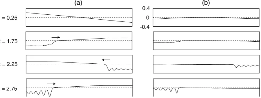
Fig. 6. Evolution of the isopycnal amplitude for (a) mode-1 and (b) mode-2 with the wind stress penetration depthhs=1.5. The abscissa

covers the full length(0,1)of the basin in the scaledx-coordinate.

The response of V1 is qualitatively similar to that in Fig. 5, but the response of V2 is quite different, exhibiting a substan-tially diminished wind energy input to V2. Hence, there is no generation of a V2 nonlinear front. Energy transfer from V1 to V2 during wave reflection is still clearly observed.

It is instructive to define the modal energy and to quantify aspects of the modal energetics. From the Euler and continu-ity equations in the Boussinesq limit, one can show (e.g., see Gerkema, 2003) that the conserved energy density is dE=1

2(u

2_+w2₎₊

∞

X n=0

Bn (n+2)!

σn+2

N2 , (36)

where

B0=1; Bn+1= −

_B n N2_(z)

z

. (37)

The energy density given in Eq. (36) has the familiar struc-ture as a sum of kinetic energy and potential energy. How-ever, the potential energy is expressed by an infinite series. For a reasonable calculation of the energy, we define the to-tal energy in the system with a variable buoyancy frequency by the integral relation

E=

Z

x Z

z ₁

2

u2+w2 +1

2 σ2 N2

+ 1

6(N

2₎0σ3 N6

)

dzdx, (38) where only a leading order correction of the potential energy for non-uniformN2(z)is included. Field variables are ex-pressed by using two vertical modes:

u=U φ₁0 +V φ₂0, w=Uxφ1+Vxφ2,

σ =N2(Y φ1+Zφ2).

(39)

Substituting Eq. (39) into Eq. (38), and evaluating the in-tegral assuming the lake depth is uniform, one obtains:

E=

( 1 2

I1

c₁2 h

hU2i +d11hUx2i +d12hUxVxi

i

+1

2 h

I1(hY2i −c21σ111hY3i)

+ I2(ν211−2σ211)hZY2i

io

V1

+

( 1 2

I2

c₂2 h

hV2i +d22hVx2i +d21hUxVxi i

+1

2 h

I2(hZ2i −c22σ222hZ3i)

+I1(ν122−2σ122)hY Z2i

io

V2, (40)

whereh· · ·idenotes integration over the horizontal domain, and all coefficients are related to coefficients in Eqs. (28– 31). Terms in Eq. (40) are selectively grouped into V1 or V2. In each group, the first bracketed term represents the kinetic energy and the last bracketed term represents the potential energy.

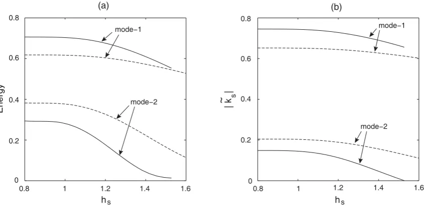
Using Eq. (40), modal energies were calculated at the end of wind forcing (t=1/4) as a function ofhs, and results are exhibited in Fig. 7.

(b)

~

0.8 1 1.2 1.4 1.6

0 0.2 0.4 0.6 0.8

hs

Energy

mode−1

mode−2

0.8 1 1.2 1.4 1.6

0 0.2 0.4 0.6 0.8

hs

| k

s

|

(a)

mode−1

mode−2

Fig. 7. (a) Modal energies and (b) modal forcing coefficients as a function of the wind stress penetration depthhs for the metalimnion

thicknessh2=1 (solid line) andh2=2 (dash line). (h3=3,W=1.5)

the wind energy is not injected to V2 directly. Energy of V2 does not vanish completely, however, because energy is still transferred from V1 to V2 during the wind forcing through nonlinear coupling. In Fig. 7, corresponding results for thick metalimnion (hs=2) are also presented. Their trends are the same as those of former case, but the decrease in modal ener-gies ashsincreases is slower. Although it is not shown in the figure, the forcing factor| ˜ks|vanishes as the wind stress pen-etration increases to near the half-depth of the metalimnion. Modal energy partition becomes more sensitive as the metal-imnion becomes thinner.

In Eq. (40), the most interesting terms arehZY2i in V1 andhY Z2iin V2. These terms are the correlation between the potential energy of one mode and isopycnal amplitude of another mode. We call these terms the energy transfer terms. Of course, energy transfer is processed through ‘all’ depen-dent variables which are governed by the evolution equa-tion set, but the energy transfer terms solely provide explicit modal energy exchange among all the other energy terms in Eq. (40). Another type of the modal interactionhUxVxi with non-hydrostatic coupling coefficients (i.e.,d12andd21)

can be equally distributed to both modes (note the identity (c2₁/I1)d12=(c₂2/I2)d21in Eq. 40), hence there is no explicit

energy transfer through this term. Here we define, for conve-nient quantification purposes, the amount of explicit modal energy transfer Et r as a difference of the energy transfer terms

Et r = 1 2α1hZY

2_{i −} 1

2α2hY Z

2_{i, (41)}

whereα1andα2are abbreviated representations of the

en-ergy transfer coefficients

α1=I2(ν211−2σ211); α2=I1(ν122−2σ122). (42)

We interpret that ifEt r>0, the amount of energy|Et r|is transferred from V2 to V1, and vice versa forEt r<0.

Figure 8 shows modal energies andEt r as a function of time forh2=1 andh2=2 withhs=1.

Energies are normalized by the total energy at the end of forcing (t=1/4). The total energy is not necessarily con-served after the wind forcing, because Eq. (40) is still an ap-proximation, and the evolution model includes bottom fric-tion damping. Fluctuafric-tion amplitudes of the total energy for h2=1 is larger than that forh2=2. This quite probably occurs

because the nonlinearity of the evolution model for a thinner metalimnion is larger, requiring a higher-order correction in the energy expression. Looking at theh2=2 case, energy

damping due to the bottom friction is negligible. Total energy for theh2=1 case seems slightly damped due to the

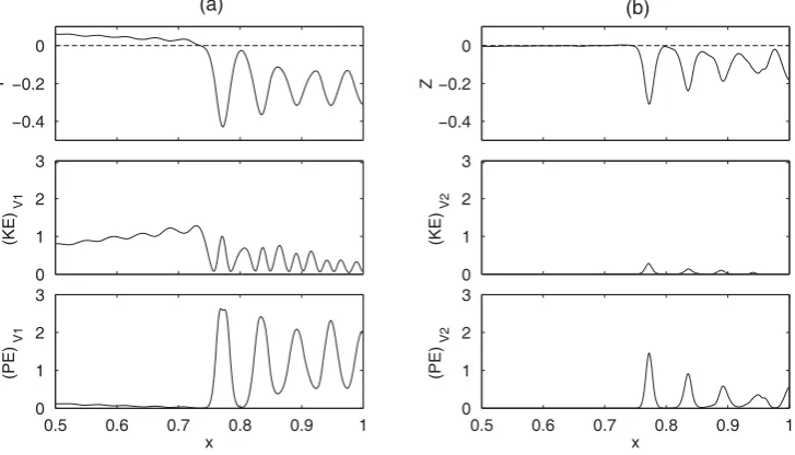
numer-ical filtering to suppress high wave number noises that arise from larger nonlinearity of V2. In all cases, the modal ener-gies oscillate in time, and they are out of phase. The amount of energy transfer also oscillates in every half V1 seiche pe-riod. Furthermore, the energy is transferred from V1 to V2 for most of the time (Et r<0). Comparing with Fig. 5, the energy transfer occurs when V1 waves reflect against the end walls, leaving their footprints in V2 domain. When V1 waves leave the wall after the reflection, the energy transferred into V2 during reflection is returned to V1, with no permanent energy transfer between the modes. Figure 9 shows verti-cally integrated potential and kinetic energy densities of each mode during V1 wave reflection at the right end wall (x=1). We chosehs=1.5 withh2=1 to focus more particularly

0 0.5 1 1.5 2 2.5 3 0

0.2 0.4 0.6 0.8 1 1.2

t

Energy

total

mode−1

mode−2

0 0.5 1 1.5 2 2.5 3

−0.12 −0.1 −0.08 −0.06 −0.04 −0.02 0 0.02

t

Etr to mode−1

to mode−2

0 0.5 1 1.5 2 2.5 3

0 0.2 0.4 0.6 0.8 1 1.2

t

Energy

total

mode−1

mode−2

0 0.5 1 1.5 2 2.5 3

−0.12 −0.1 −0.08 −0.06 −0.04 −0.02 0 0.02

t

Etr

to mode−1 to mode−2

(a) (b)

Fig. 8. Modal energies (upper row) and corresponding energy transferEt r(lower row) as a function of time for (a)h2=1 and (b)h2=2. (W=1.5,hs=1,h1+h2+h3=5).

−0.4 −0.2 0

Y

−0.4 −0.2 0

Z

0 1 2 3

(KE)

V1

0 1 2 3

(KE)

V2

0.5 0.6 0.7 0.8 0.9 1 0

1 2 3

(PE)

V1

x

0.5 0.6 0.7 0.8 0.9 1 0

1 2 3

(PE)

V2

x

(a) _(b)

Fig. 9. The isopycnal amplitude (upper row), kinetic energy density (middle row) and potential energy density (bottom row) att=3.25 over the right half domain for (a) mode-1 and (b) mode-2. Energies are normalized by the total system energy. (h2=1,h3=3,W=1.5,hs=1.5)

than a factor of two. In the V2 packet, the potential energy is much larger than the kinetic energy which is almost negli-gible. During V1 wave reflection, the potential energy of V1 dominates near the end wall, because the isopycnal ampli-tude increases due to superposition of incident and reflected

waves and, also, the horizontal velocity (kinetic energy) ap-proaches zero at the end wall. The dominance of potential energy in V1 is preferably transferred to V2.

Table 4. The modal energyEt rtransferred from vertical mode-1 to

mode-2 and the energy transfer coefficientsα1andα2for various

h2,Nh2andh3(W=1.5.)

Et r Et r h2 Nh2 h3 α1 α2 (hs=1) (hs=1.5)

1 0 3 1.387 0.262 0.120 0.113

1.5 0 3 1.206 0.318 0.041 0.037

2 0 3 0.999 0.302 0.017 0.016

3 0 3 0.506 0.000 0.004 0.004

1 0.1 3 0.582 −0.012 0.049 0.035

1 0.2 3 0.293 −0.108 0.016 0.011

1 0.5 3 0.084 −0.195 0.002 0.002

1 0 1 1.210 0.000 0.058 0.045

1 0 2 1.351 0.196 0.095 0.083

1 0 4 1.396 0.294 0.138 0.136

coefficients (α1andα2) are tabulated for various sets ofh2,

N_h2,h3andhs.

The energy transfer becomes larger for smallerh2orN_h2,

as indicated by the fact thatα1becomes much larger thanα2.

Values ofα1are much larger thanα2for all choices ofh3,

in-dicating a dominance of energy transfer from V1 to V2. The coefficientsν211andσ211inα1arise from the vertical

inte-gral of the buoyancy flux terms (σ uandσ w) of V1, which are coupled in the V2 evolution equation (Eq. 30).ν211arises

from the vertical buoyancy flux (σ w), andσ211arises form

the horizontal buoyancy flux (σ u). As seen in Table 1–3,ν211

is much larger thanσ211. This implies that the vertical

buoy-ancy flux of V1 plays an important role in transferring en-ergy from V1 to V2. Especially, a thinner metalimnion cor-responds to largerν211, resulting in more pronounced energy

transfer to V2. It can also be observed from Table 4 that wind stress penetration into the metalimnion gives little change in the amount of energy transfer. In Fig. 10 we show the amount of energy transfer from V1 to V2 as a function of the Wed-derburn number for selected profiles of buoyancy frequency. The fractional amount of energy transfer increases quadrati-cally with respect to the inverse of the Wedderburn number for all cases.

5 Discussions

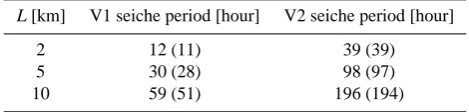
In order to provide some insight as to nominal time scales one might encounter in applications, we present in Table 5 data for the V1 and V2 seiche periods in lakes with a Brunt-V¨ais¨al¨a frequency of 0.02 [s−1] in the metalimnion, and with respective depth and length scales as given. The seiche pe-riod for V1 is the normalizing time scale for dynamics shown in Fig. 5, and in all following figures. It is evident that the V2 seiche period is typically a factor of three or four times longer

0.2 0.4 0.6 0.8 1 1.2

0 0.1 0.2 0.3

W−1

Etr

h₂= 1, N_h2= 0

h₂= 1, N_h2 = 0.1

h₂= 2, N_h2 = 0

Fig. 10. Modal energy transferEt r (from mode-1 to mode-2) as a

function of inverse Wedderburn numberW−1for different stratifi-cation profiles. (h3=3,hs=1.5)

Table 5. Mode-1 (V1) and mode-2 (V2) seiche periods for different

lake lengthsLwithh1=5 [m],h2=h1, h3=3h1,N0=0.02 [s−1],

Nh=0 andδ=0.1. Values in parenthesis are for thicker hypolimnion

withh3=5h1. Each of the seiche periods is defined as 2Ldivided by the respective eigenspeed (cn).

L[km] V1 seiche period [hour] V2 seiche period [hour]

2 12 (11) 39 (39)

5 30 (28) 98 (97)

10 59 (51) 196 (194)

than that of V1. However, the nonlinear steepening of the V2 front arising from a wind event clearly occurs much earlier in time than does the steepening of the V1 front. As a conse-quence, the self-modal nonlinear interaction of V2 is contin-ually propagating through a variable background formed by the larger-scale V1 field. Sustained wind for periods on the order of one-eight to one-half V1 seiche period leads to sig-nificant energy deposited into the basin-scale internal wave field, which subsequently cascades to smaller scales through process studied here.

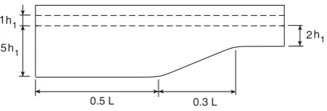
0.5 L 0.3 L

2 5

1

h₁

h₁

h₁

Fig. 11. Sloping depth configuration.

penetration of the wind stress in conjunction with the verti-cal stratification profile determines the initial energy input to each vertical mode.

Recently, Stashchuk et al. (2005) conducted numerical experiments to simulate the fully-nonlinear, baroclinic re-sponse of a near two-layer fluid in a rectangular, long, narrow tank, an experimental configuration similar to that employed by Horn et al. (2001). Stashchuk et al. (2005) discovered that the metalimnion (interfacial) layer thickens behind the nonlinear wave front (see Figs. 6 and 7 in their paper). They concluded that the layer thickening is attributed to the inter-action of the wave front with the vertical side walls (see Fig. 8 in their paper). They did not conclude that the widening is at-tributed to V2, due to the fact that the field velocity profile did not comply with typical V2 eigenprofiles. However, V1 and V2, or even higher vertical modes, can coexist in the field, and they are superimposed, at least in a linear sense. This requires a decomposition of the disturbance field into verti-cal modes, which indeed the present multi-modal approach does, to determine the modal energy spectrum. Their results exhibited that the widening part of the density layer persis-tently follows the tail of the nonlinear wave train. If this layer widening is attributed to V2, this phenomenon implies the permanent energy transfer from V1 to V2, which is not observed in the model simulations presented here. Their den-sity layer is very thin (about 0.2h1), and the initial V1 wave

amplitude is large (0.9h1). This configuration, however, is

outside the operational range of the present weakly-nonlinear model.

Although the variable depth terms in the evolution model admit modal energy transfer, our model simulations exhib-ited that inter-mode transfer is negligible in variable depth cases. For example, Fig. 12 shows evolution of isopycnal amplitudes in a lake having a sloping topography as depicted in Fig. 11.

Wind stress penetration depth was chosen to behs=1.5 to suppress energy input to V2 in order to see modal interaction during V1 waves propagating over the sloping bottom. At t=3, V1 waves are about to pass over the slope, but at this time no significant interaction is observed in the V2 packet. Modal interaction during V1 wave reflection is rather out-standing as observed att=2.75 andt=3.25. In Fig. 13, cor-responding pictures for the uniform depth configuration are shown.

Table 6. Coefficients of variable topography terms for different

val-ues of the slope heighth3s.

h3s 1 2 3 4

κ11 0.178 0.414 0.730 1.155

κ12 −0.015 −0.037 −0.070 −0.119

λ11 0.014 0.031 0.048 0.058

λ12 −0.361 −0.879 −1.643 −2.810

κ21 0.002 0.005 0.010 0.017

κ22 0.003 0.007 0.014 0.023

λ21 −0.021 −0.052 −0.101 −0.178

λ22 0.012 0.027 0.049 0.078

κ12/κ11 −0.09 −0.09 −0.10 −0.10

λ12/λ11 −25.4 −28.6 −34.4 −48.9

κ21/κ22 0.71 0.72 0.73 0.75

λ21/λ22 −1.82 −1.92 −2.05 −2.27

Wave amplitudes are larger than the former case because the wind forcing factorksnand nonlinearity are larger in the uniform depth case. It can be observed that there are a se-ries of small footprints of the V1 oscillatory waves in the V2 domain, but the V1 wave reflection contributes a much larger footprint to the V2 domain. Qualitative structures of the modal components of the wave field in the variable depth case and the uniform counterpart are still very similar.

The weak cross-modal transfer due to varying depth was explored further by examining the coefficientsκijandλij ap-pearing in Eqs. (28–31) for a range of topographic slopes. Using a linear slope prescribed by h3=h30−(h3s/ ls)x, where h30, h3s andls are the maximum depth of the hy-polimnion, the change in hypolimnion depth, and the hor-izontal length of the slope, respectively, coefficient values were computed and presented in Table 6. The coefficient val-ues shown pertain to a configuration withh30=5h1,ls=L/3, h2=h1, andN_h2=0. Furthermore, coefficient values are

re-ported at the mid-slope depth position (i.e., atxs=ls/2). One notes that the coefficient values in Table 6 are significantly less than unity, except for the self modal coefficientκ11

ap-pearing in the V1 velocity evolution equation Eq. (28), and for the cross modal coefficientλ12appearing in the V1

t = 2.75

t = 3

t = 3.25

t = 3.5

0.5

-0.5

(a)

(b)

0

Fig. 12. Isopycnal amplitudes of (a) mode-1 and (b) mode-2 over sloping topography at different time (W=1.5,hs=1.5). The abscissa

covers the full length(0,1)of the basin in the scaledx-coordinate.

t = 2.75

t = 3

t = 3.25

t = 3.5

0.5

-0.5

(a)

(b)

0

Fig. 13. Isopycnal amplitudes of (a) mode-1 and (b) mode-2 over uniform topography (h₃=5) at different time (W=1.5,hs=1.5). The

abscissa covers the full length(0,1)of the basin in the scaledx-coordinate.

6 Conclusions

A multi-modal, weakly-nonlinear model for the wind-forced response of basin-scale internal waves in an inhomogeneous environment was derived. The two-vertical-mode interac-tion was investigated by numerically simulating the evolu-tion model for several modeled Brunt–V¨ais¨al¨a profiles and several wind forcing functions. Energy distribution among the modes was studied by defining modal energy and energy transfer functions in truncated form.

Initial modal energy partition right after uniform wind forcing of specified duration strongly depends on vertical structures of both the stratification and the wind stress. Pen-etration of the wind stress into the metalimnion can signifi-cantly change the modal energy input, especially for mode-2 and for a thin metalimnion. Determining the initial modal

en-ergy partition following wind setup is very important because the subsequent evolution (especially mo2) is strongly de-pendent on the modal energy input.

to mode-2. Thin metalimnion configurations increase the vertical buoyancy flux of mode-2 that is induced by mode-1 via nonlinear modal coupling, enhancing the energy transfer from mode-1 to mode-2.

Edited by: R. Grimshaw

Reviewed by: two anonymous referees

References

Antenucci, J., Imberger, J., and Saggio, A.: Seasonal evolution of the basin-scale internal wave field in a large stratified lake, Lim-nol. Oceanogr., 45(7), 1621–1638, 2000.

Baines, P. G.: Topographic effects in strafified flows, Cambridge University press, 47–48, 1995.

Boehrer, B.: Modal response of a deep stratified lake: western Lake Constance, J. Goephys. Res., 105, 28837–28845, 2000. Bogucki, D. J., Redekopp, L. G., and Barth, J.: Internal

soli-tary waves in the coastal mixing and optics 1999 experiment: multimodal structure and resuspension, J. Geophys. Res., 110, doi:10.1029/2003JC002253, 2005.

Gerkema, T.: Internal and interfacial tides: beam scattering and local generation of solitary waves, J. Mar. Res., 59, 227–255, 2001.

Gerkema, T.: Development of internal solitary waves in vari-ous thermocline regines - a multi-modal approach, Nonlin. Pro-cessess. Geophys., 10, 397–405, 2003.

Griffiths, S. D. and Grimshaw, R. H. J.: Internal tide generation at the continental shelf modeled using a modal decomposition: two dimensional results, J. Phys. Oceanogr., 37, 428–451, 2007. Grimshaw, R. (ed.): Internal solitary waves, Kluwer Academic

Pub-lishers, in: Environmental stratified flows, 12–14, 2002. Heaps, N. S. and Ramsbottom, A. E.: Wind effects on the water in a

narrow two-layered lake, Phil. T. R. Soc. Lond. A, 259, 391–430, 1966.

Horn, D. A., Imberger, J., and Ivey, G. N.: The degeneration of large-scale interfacial gravity waves in lakes, J. Fluid Mech., 434, 181–207, 2001.

H¨uttemann, H. and Hutter, K.: Boroclinic solitary waves in a two-layer fluid system with diffusive interface, Exp. Fluids, 30, 317– 326, 2001.

Imberger, J. and Patterson, J. C.: Physical Limnology, Adv. Appl. Mech., 27, 303–475, 1990.

LaZerte, B. D.: The dominating higher order vertical modes of the internal seiche in a small lake., Limnol. Oceanogr., 25, 846–854, 1980.

Lele, S.: Compact finite difference schemes with spectral-like reso-lution, J. Comput. Phys., 103, 16–42, 1992.

Monismith, S.: Modal response of reservoirs to wind stress, J. Hy-draul. Eng., 113, 1290–1306, 1987.

Mortimer, C. H.: Water movements in lakes during summer strati-fication; evidence from the distribution of termperature in Win-dermere, Phil. Trans. Roy. Soc. London, B, 236, 355–404, 1952. M¨unnich, M., W¨uest, A., and Imboden, D. M.: Observations of the second vertical mode of the internal seiche in an alpine lake, Limnol. Oceanogr., 37, 1705–1719, 1992.

Phillips, O. M.: The dynamics of the upper ocean, Cambridge uni-versity press, 139–145, 1966.

Roget, E., S. G. and Zamboni, F.: Internal seiche climatology in a small lake where transversal and second vertical modes are usu-ally observed, Limnol. Oceanogr., 42, 663–673, 1997.

Slinn, D. N. and Riley, J. J.: A model for the simulation of turbulent boundary layers in an incompressible stratified flow, J. Comput. Phys., 144, 550–602, 1998.

Stashchuk, N., Vlasenko, V., and Hutter, K.: Numerical modelling of disintegration of basin-scale internal waves in a tank filled with stratified water, Nonlin. Processes Geophys., 12, 955–964, 2005,

http://www.nonlin-processes-geophys.net/12/955/2005/. Vlasenko, V. and Hutter, K.: Generation of second mode solitary

waves by the interaction of a first mode soliton with a sill, Nonlin. Processes Geophys., 8, 223–239, 2001,

http://www.nonlin-processes-geophys.net/8/223/2001/.