Q-Format Data Representation and Its Arithmetic

(1)

57

Q-Format Data Representation and Its Arithmetic

1

Md. Zakir Hussain,

2

Kazi Nikhat Parvin

1_{Dept. of ECE, Muffakham Jah college of Engineering and Technology, Hyderabad, Telangana, India}

2_{Dept. of ECE, Bhoj Reddy Engineering College for Women, Saidabad, Hyderabad, Telangana, India}

Abstract

In the early days of computing, there were common misconceptions about computers. One misconception was that the computer was only a giant adding machine performing arithmetic operations. Computers could do much more than that, even in the early days. The other common misconception, in contradiction to the first, was that the computer could do “anything.” We now know that there are indeed classes of problems that even the most powerful imaginable computer finds intractable with the von Neumann model. The correct perception, of course, is somewhere between the two.

We might think of the decimal representation of information as the most natural when we know it the best, but the use of on-off codes to represent information predated the computer by many years, in the form of Morse code.

This section introduces several of the simplest and most important encodings: the encoding of signed and unsigned fixed point numbers, real numbers (referred to as floating point numbers in computer jargon), and the printing characters. We shall see that in all cases there are multiple ways of encoding a given kind of data, some useful in one context, some in another.

Keywords

Q-point, Floating-point, Fixed-point, Computer Arithmetic.

I. Fixed Point Numbers

In a fixed point number system, each number has exactly the same number of digits, and the “point” is always in the same place. Examples from the decimal number system would be 0.23, 5.12, and 9.11. In these examples each number has 3 digits, and the decimal point is located two places from the right. Examples from the binary number system (in which each digit can take on only one of the values: 0 or 1) would be 11.10, 01.10, and 00.11, where there are 4 binary digits and the binary point is in the middle. An important difference between the way that we represent fixed point numbers on paper and the way that we represent them in the computer is that when fixed point numbers are represented in the computer the binary point is not stored anywhere, but only assumed to be in a certain position. One could say that the binary point exists only in the mind of the programmer.

We begin coverage of fixed point numbers by investigating the range and precision of fixed point numbers, using the decimal number system. We then take a look at the nature of number bases, such as decimal and binary, and how to convert between the bases. With this foundation, we then investigate several ways of representing negative fixed point numbers, and take a look at simple arithmetic operations that can be performed on them.

A. Range and Precision in Fixed Point Numbers

A fixed point representation can be characterized by the range of expressible numbers (that is, the distance between the largest and smallest numbers) and the precision (the distance between two adjacent numbers on a number line.) For the fixed-point decimal example above, using three digits and the decimal point placed two digits from the right, the range is from 0.00 to 9.99 inclusive of the endpoints, denoted as [0.00, 9.99], the precision is .01, and

the error is 1/2 of the difference between two “adjoining” numbers, such as 5.01 and 5.02, which have a difference of .01. The error is thus .01/2 = .005. That is, we can represent any number within the range 0.00 to 9.99 to within .005 of its true or precise value. Notice how range and precision trade off: with the decimal point on the far right, the range is [000, 999] and the precision is 1.0. With the decimal point at the far left, the range is [.000, .999] and the precision is .001.

In either case, there are only 103 different decimal “objects,” ranging from 000 to 999 or from .000 to .999, and thus it is possible to represent only 1,000 different items, regardless of how we apportion range and precision.

There is no reason why the range must begin with 0. A 2-digit decimal number can have a range of [00, 99] or a range of [-50, +49], or even a range of [-99, +0].

Range and precision are important issues in computer architecture because both are finite in the implementation of the architecture, but are infinite in the real world, and so the user must be aware of the limitations of trying to represent external information in internal form.

B. An Early Look at Computer Arithmetic

We will explore computer arithmetic, but for the moment, we need to learn how to perform simple binary addition because it is used in representing signed binary numbers. Binary addition is performed similar to the way we perform decimal addition by hand. Two binary numbers A and B are added from right to left, creating a sum and a carry in each bit position. [5]

Since the rightmost bits of A and B can each assume one of two values, four cases must be considered: 0 + 0, 0 + 1, 1 + 0, and 1 + 1, with a carry of 0, as shown in the figure. The carry into the rightmost bit position defaults to 0. For the remaining bit positions, the carry into the position can be 0or 1, so that a total of eight input combinations must be considered [7].

Notice that the largest number we can represent using the eight-bit format shown in Figure 2-5 is (11111111)₂ = (255)₁₀ and that the smallest number that can be represented is (00000000)₂ = (0)₁₀. The bit patterns 11111111 and 00000000 and all of the intermediate bit patterns represent numbers on the closed interval from 0 to 255, which are all positive numbers. Up to this point we have considered only unsigned numbers, but we need to represent signed numbers as well, in which (approximately) one half of the bit patterns is assigned to positive numbers and the other half is assigned to negative numbers. Four common representations for base 2 signed numbers are discussed in the next section.

C. Signed Fixed Point Numbers

(2)

1. Signed Magnitude

The signed magnitude (also referred to as sign and magnitude) representation is most familiar to us as the base 10 number system. A plus or minus sign to the left of a number indicates whether the number is positive or negative as in +12₁₀ or -12₁₀. In the binary signed magnitude representation, the leftmost bit is used for the sign, which takes on a value of 0 or 1 for ‘+’ or ‘-’, respectively. The remaining bits contain the absolute magnitude. Consider representing (+12)₁₀ and (-12)₁₀ in an eight-bit format:

The negative number is formed by simply changing the sign bit in the positive number from 0 to 1. Notice that there are both positive and negative representations for zero: 00000000 and 10000000. There are eight bits in this example format, and all bit patterns represent valid numbers, so there are 28_{= 256 possible patterns.}

Only 28 - 1 = 255 different numbers can be represented, however, since +0 and -0 represent the same number.

We will make use of the signed magnitude representation when we look at floating point numbers.

2. One’s Complement

The one’s complement operation is trivial to perform: convert all of the 1’s in the number to 0’s, and all of the 0’s to 1’s. For examples we can observe from the table that in the one’s complement representation the leftmost bit is 0 for positive numbers and 1 for negative numbers, as it is for the signed magnitude representation. This negation, changing 1’s to 0’s and changing 0’s to 1’s is known as complementing the bits. Consider again representing (+12)₁₀ and (-12)₁₀ in an eight-bit format, now using the one’s complement representation:

Note again that there are representations for both +0 and -0, which are 00000000 and 11111111, respectively. As a result, there are only 28 - 1 = 255 different numbers that can be represented even though there are 28 different bit patterns.

The one’s complement representation is not commonly used. This is at least partly due to the difficulty in making comparisons when there are two representations for 0. There is also additional complexity involved in adding numbers.

3. Two’s Complement

The two’s complement is formed in a way similar to forming the one’s complement: complement all of the bits in the number, but then add 1, and if that addition results in a carry-out from the most significant bit of the number, discard the carry-out.In the two’s complement representation, the leftmost bit is again 0 for positive numbers and is 1 for negative numbers.

However, this number format does not have the unfortunate characteristic of signed-magnitude and one’s complement representations: it has only one representation for zero. To see that this is true, consider forming the negative of (+0)₁₀, which has the bit pattern:

(+0)₁₀ = (00000000)₂

Forming the one’s complement of (00000000)₂ produces (11111111)₂ and adding 1 to it yields (00000000)₂, thus (-0)₁₀ = (00000000)₂. The carry out of the leftmost position is discarded in two’s complement addition (except when detecting an overflow condition). Since there is only one representation for 0, and since all bit patterns are valid, there are 28 = 256 different numbers that can be represented.

Consider again representing (+12)₁₀ and (-12)₁₀ in an eight-bit format, this time using the two’s complement representation. Starting with (+12)₁₀ = (00001100)₂, complement, or negate the number, producing (11110011). Now add 1, producing

(11110100)₂, and thus (-12)₁₀ = (11110100)₂: (+12)₁₀ = (00001100)₂

(-12)₁₀ = (11110100)₂

There is an equal number of positive and negative numbers provided zero is considered to be a positive number, which is reasonable because its sign bit is 0. The positive numbers start at 0, but the negative numbers start at -1, and so the magnitude of the most negative number is one greater than the magnitude of the most positive number. The positive number with the largest magnitude is +127, and the negative number with the largest magnitude is -128.

There is thus no positive number that can be represented that corresponds to the negative of -128. If we try to form the two’s complement negative of -128, then we will arrive at a negative number, as shown below:

The two’s complement representation is the representation most commonly used in conventional computers, and we will use it throughout the book [6]

II. Arithmetic Operations

The basic arithmetic operations on fixed-point numbers, addition, subtraction, multiplication, and division, are operations with two inputs (the operands) and one output (the result). These operators are usually denoted binary operators. They can be implemented using ordinary integer arithmetic operations and bit shifting. The bit shifts (left shift and right shift) of an integer number q are (q ≪ n) = q.2n

and

(q ≫ n) = [q. 2-n_]

Note that only the integer part of the result is kept and the remainder is discarded. This means that we lose information and errors are introduced.

Furthermore, the operation is compiler dependent for signed integers taking a negative value [10], so care has to be taken choosing a compiler that interpret right shift as defined above, otherwise obscure and hard-to-trace errors may be introduced. Bit shifting is a fast operation that is used extensively to rescale both the inputs of an operation and the output.

An additional note is that since the implementation of right shift is compiler dependent one can generate code for an integer division with the corresponding power of two instead and let the compiler optimize the code.

A. Addition

Addition of two fixed-point variables Q₁ and Q₂on the form Q[m₁, n₁] and Q[m₂, n₂] can be described by finding Q such that Q=Q₁ +Q₂

In order to add Q₁and Q₂, the binary points must be aligned. This can be done if both Q₁ and Q₂have the same number of fractional bits, n₁= n₂. Aligned binary points, n₁= n₂

If the binary-points are aligned, the two variables can be added, assuming that the result is not larger than the representation can handle. If the binary points are not aligned, then one or more of the operands must be shifted before the addition can be performed. The different cases are discussed in more detail below.

When n₁= n₂ =n the two variables can be added according to Q = Q₁+Q₂

and Q will have the same number of fractional bits as the operands. The integer part of Q can be stored using max(m₁, m₂) + 1bits. As a motivating example consider the “worst case” when Q₁=Q ₂. Then

(3)

59

B. Subtraction

Subtraction of two fixed-point variables Q₁ and Q₂on the form Q[m₁, n₁] and Q[m₂, n₂] can be described by finding Q such that

Q=Q₁ -Q₂

In order to add Q₁ and Q₂, the binary points must be aligned. This can be done if both Q₁ and Q₂ have the same number of fractional bits, n₁= n₂. Aligned binary points, n₁= n₂

When n₁=n₂=n the two variables can be subtracted according to Q=Q₁-Q₂

And Q will have the same number of fractional bits as the operands. The integer part of Q can be stored using max(m₁, m₂) + 1 bits. As a motivating example consider the “worst case” when Q₁=Q ₂. Then

Q₁-Q₂=Q₁-Q₁=0

C. Multiplication

Multiplication of two fixed-point variables Q₁and Q₂ on the form Q₁[m₁,n₁], Q₂[m₂,n₂] gives a result on the form Q[m₁ + m₂ + 1, n₁ + n₂]. We split multiplication in two cases; the result can be stored and the result is too big to store.

The first case is trivial, just multiplying the factors and getting a result on the form Q[m₁ + m₂ + 1, n₁ + n₂]. This result could then be rescaled if needed to remove a portion of the least significant bits. A common choice is to truncate the result so that is does not have more fractional bits than any of the factors. As before note that we need m + n + 1 bits to store Q[m,n] and thus we need m₁ + m₂ + n₁ + n₂ + 2bits to store the multiplication [5].

D. Division

1. Restoring Division

A shift register keeps both the (remaining) dividend as well as the quotient with each cycle, dividend decreases by one digit & quotient increases by one digit the MSB’s of the remaining dividend and the divisor are aligned in each cycle major difference to multiplication:

We do not know if we can subtract the divisor or not •

If the subtraction failed, we have to restore the original •

dividend 226 Sequential Restoring Division 1. Load the 2n dividend into both halves of shift register, and add a sign bit to the left 2. add a sign bit to the left of the divisor

generate the 2’s complement of the divisor •

shift to the left •

add 2’s complement of the divisor to the upper half of the •

shift register including sign bit (subtract)

if sign of the result is cleared (positive) then set LSB of the •

lower half of the shift register to one else clear LSB of the lower half and add the divisor to upper half of shift register (restore)

Repeat from 4 and perform the loop n times after •

termination

III. Algorithms and Flow Graphs A. Addition Flow Graph

Fig. 1: Flow Graph of Addition

Addition of two fixed-point variables Q₁ and Q₂on the form Q[m₁, n₁] and Q[m₂, n₂] can be described by finding Q such that

Q=Q₁ +Q₂

In order to add Q₁and Q₂, the binary points must be aligned. This can be done if both Q₁ and Q₂have the same number of fractional bits, n₁= n₂. Aligned binary points, n₁= n₂

When n₁= n₂ =n the two variables can be added according to Q=Q₁+Q₂

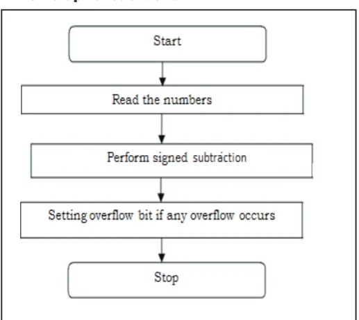
B. Flow Graph of Subtraction

(4)

Subtraction of two fixed-point variables Q₁ and Q₂on the form Q[m₁,n₁] and Q[m₂,n₂] can be described by finding Q such that Q=Q₁ - Q₂

In order to sub Q₁and Q₂, the binary points must be aligned. This can be done if both Q₁ and Q₂have the same number of fractional bits, n₁= n₂. Aligned binary points, n₁= n₂

If the binary-points are aligned, the two variables can be subtracted, assuming that the result is not larger than the representation can handle. If the binary points are not aligned, then one or more of the operands must be shifted before the addition can be performed. The different cases are discussed in more detail below.

When n₁= n₂ =n the two variables can be added according to Q = Q₁-Q₂

C. Flow Graph of Multiplication

Fig. 3: Flow Graph of Multiplication

Multiplication of two numbers can be done by reading two number and performing signed multiplication and integer part and fractional part can be adjusted in defined q-format

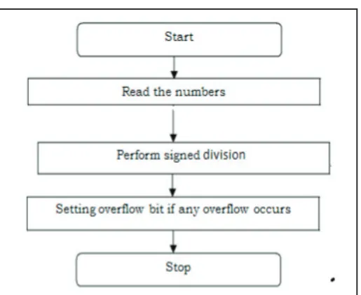
D. Flow Grpah of Division

Fig. 4: Flow Grpah of Division

Division of two numbers can be done in sequential manner by performing read operation at positive edge clock and performing division setting overflow if there is an overflow and complete will be high at the end of the result.

IV. Simulation Results A. Fixed Point Arithmetics 1. Q-Addition

Example 1:When both a and b are positive

a=2.1=00000000000000010000110011001100 b=3.5 =00000000000000011100000000000000 c=a+b=5.6=000000000000001011001100110011000

Fig. 5: Simulation Result of Addition

In the above data representation, the LSB part is signed bit, followed by 16 integer bit and then followed by 15 fractional bit to give a total of 32 bit number.

In the above example, ‘a’ and ‘b’ are two fixed point inputs and ‘c’ is the output of addition of a and b. Since both the inputs are positive therefore output of a and b is positive

Example 2: When both a and b are negative

a=-2.1=10000000000000010000110011001100 b=-3.5 =10000000000000011100000000000000 c=a+b=-5.6=10000000000000101100110011001100

Fig. 6: Simulation Result of Addition

In the above example, ‘a’ and ‘b’ are two fixed point inputs and ‘c’ is the output of addition of a and b. Here a and b are negative numbers, so addition of two negative numbers is always negative , therefore the signed bit of the output c is high.

Q-Subtraction:

Example 1: When both a and b are positive

(5)

61

Fig. 7: Simulation Result of Subtraction

In the above example, ‘a’ and ‘b’ are two fixed point inputs and ‘c’ is the output of subtraction of a and b. Since both the inputs are positive therefore output of a and b is positive.

a=-27.8=10000000000011011110011001100110 b=-19.6 =10000000000010011100110011001100 c=a-b=-8.2=10000000000001000100001101001111

Fig. 8: Simulation Result of Subtraction

In the above example, ‘a’ and ‘b’ are two fixed point inputs and ‘c’ is the output of subtraction of a and b. Here a and b are negative numbers, so subtraction of of two negative numbers is always negative, therefore the signed bit of the output c is high.

3. Q-Multiplication

Example 1:When both a and b are positive

a=10.7=00000000000001010101100110011001 b=14.2 =00000000000001110001100110011001 c=a*b=151.94=00000000010010111110110011100011

Fig. 9: Simulation Result of Multiplication

Multiplication requires double wordlength to store the intermediate values of multiplication operation.

In the above example, ‘a’ and ‘b’ are two fixed point inputs and ‘e’ is the output of multiplication of a and b. The multiplication operation starts when the start bit is high and the clk high at the positive edge. The operation is completed when the complete1 bit is high.

a=-10.7=10000000000001010101100110011001 b=-14.2 =10000000000001110001100110011001 c=a*b=151.94=00000000010010111110110011100011

Fig. 10: Simulation Result of Multiplication

In the above example, ‘a’ and ‘b’ are two fixed point inputs and ‘e’ is the output of multiplication of a and b. The multiplication operation starts when the start bit is high and the clk high at the positive edge. The operation is completed when the complete1 bit is high.

Here a and b are negative numbers, so the multiplication of two negative numbers is always positive , therefore the signed bit of the output e is low.

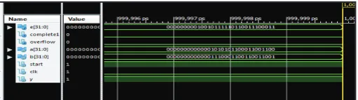
4. Q-Division:

Example 1: When both a and b are positive

dividend=8.8=00000000000001000110010011001100 divisor=2.2 =00000000000000010001100110011100

quotientout=a/b=4=00000000000000100000000000000000

Fig. 11: Simulation Result of Division

Division like multiplication requires double wordlength to store the intermediate values of multiplication operation.

In the above example, ‘dividend’ and ‘divisor’ are two fixed point inputs and ‘quotientout’ is the output of division of a and b. The division operation starts when the start bit is high and the clk high at the positive edge. The operation is completed when the complete bit is high.

V. Conclusion

(6)

The work presented in this thesis addressed the automated synthesis of certified fixed-point programs and treated the particular cases of code generation for some linear algebra basic blocks. For this purpose, it tackled two recurrent issues encountered by embedded systems developers. These issues are the difficulty of fixed-point programming and the perceived low numerical quality of fixed-point computations. This work also led to the development of software tools XILINX 14.7

Writing fixed-point programs is tedious, time consuming, and requires arithmetic proficiency. To make it accessible to non-experts, this work suggests to build fixed-point synthesis tools instead of manually developing fixed-point programs. Moreover, to make it easy to perform range and error analyses, such tools must have a clear arithmetic model.

The second issue with fixed-point numbers is their perceived lack of accuracy. This thesis tackles it by suggesting that the arithmetic model comes with strict bounds on the rounding errors of each operator

We have implemented for a fixed q format representation for 32bit. It can also be implemented for different q-formats representation and can be evaluated on matlab. The matlab code can be written and can be compared the results with Xilinx results

References

[1] Simon Haykin,“Adaptive filter theory,” Pearson Education Publication, 4th Edition, May 2012, pp. 231-278.

[2] Emmanuel Ifeachor and Barrie W. Jervis,“Digital Signal Processing,” Pearson Education Publication, 2nd Edition, Jan. 2013, pp. 342-440.

[3] Kamran Eshraghian, Douglas A. Pucknell, Sholeh Eshraghian” Essentials of VLSI Circuits and Systems, “PHI Publication, 2005.

[4] Michael D. Ciletti,“Modelling, Synthesis, and Rapid Prototyping with the VERILOG HDL”, Pearson Education Publication.

[5] R. E. Moore, “Methods and Applications of Interval Analysis,” SIAM, Philadelphia, Jun. 1979, pp. 4-27.

[6] John Pryce, “IEEE Working Group P1788, A standalone for Interval Arithmetic,” Dagastuhl Seminar 09471, Cranfield University, Nov. 2009, pp. 1-20.

[7] T. Hickey, Q. Ju, M.H. Van Emden, “Interval Arithmetic: from Principles to Implementation,” Journal of the ACM (JACM), Vol. 48 No. 5, Sep. 2001, pp. 1038-1068. [8] R. E. Moore,“Automatic Error Analysis in Dig-ital

Computation,” Technical Report No. 48421, Lockheed Missiles and Space Co., Sunnyvale, California, Jan. 1959, pp. 1-5.

[9] R. E. Moore, “Methods and Applications of Interval Analysis,” SIAM, Philadelphia, Jun. 1979, pp. 4-27.

[10] John Pryce, “IEEE Working Group P1788, A standalone for Interval Arithmetic,” Dagastuhl Seminar 09471, Cranfield University, Nov. 2009, pp. 1-20.