3470
Drug Consumption Risk Analysis
S Anjali Devi, Mukkamala Mounika, Morusu Sai Harshitha, Tumati Jaswanth
Abstract: The main objective is to determine the risk of drug consumption of individuals. This can be done based on some factors. The data set that we used consists of 1885 respondents and for each individual, we have collected scores based on their personality measurements. The individual levels of consumption of some drugs like Coke, Heroin, Amphet, Benzos are taken. We have classified individual consumption levels as Never Used, Used over a decade ago, Used in the last decade, Used in last year, Used in last month, Used in last week, Used in last day. In order to determine the consumption levels, we have used two classification algorithms namely Naïve Bayes Random Forest and Support Vector Machine (SVM).
Index Terms: Classification, Consumption, Naïve Bayes, Random Forest.
—————————— ——————————
1.
INTRODUCTION
DRUG use is the major threat that hinders the growth of our country. Drug consumption effects the health of a person. A person’s personality profile can be used to determine whether he can be a drug user on not. Personality measurements are Neuroticism, Extraversion, Openness to Experience, Agreeableness and Conscientiousness ―[2],[7]‖.
Personality measurements are as follows:
1. Neuroticism: It is a tendency to express negative emotions such as anxiety and tension.
2. Extraversion: They enjoy human interaction such as talkative and taking words of other people in a positive manner.
3. Openness to Experience: It is like appreciating some others art.
4. Agreeableness: It is a measure of interpersonal conduct such as trust and kindness.
5. Conscientiousness: It is also a tendency to be organized and strong willed ―[2],[7]‖.
So in order to determine the consumption level of an individual based on their personality scores we have used three machine learning classification techniques. A computer program is said to learn from Experience (E) with respect to some task (T) and some performance measure (P) , it performs on T as measured by P improves with experience(E) [1]. In simple words Machine Learning can be defined as a machine that can learn from its past experience. There are three types of learnings in machine learning. They are:
1. Supervised Learning, 2. Unsupervised Learning and 3. Reinforcement Learning.
The algorithms that we have used comes under supervised learning. Supervised Learning is nothing but categorising data based on prior information [3]. We have used Naïve Bayes, Random Forest and Support Vector Machine (SVM) algorithms. Each of these algorithms will be discussed in the further sections.
2
METHODOLOGY
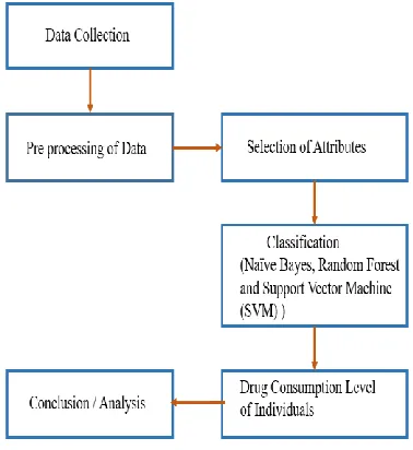
First, we have collected data on drug addiction levels of individuals based on their personality measurements. Later we performed pre-processing techniques to avoid false results. After pre-processing, the data would be free from errors and missing values. Then classification is done using Naïve Bayes, Random Forest and Support Vector Machine (SVM) algorithms. Many applications of such machine learning techniques found in literature for different applications [8-13]. After the classification we get the results. Results are represented using data visualization techniques using histogram. The reason why we have used this data visualization techniques is that it will be easily understood by the common people even if they don’t have knowledge on machine learning techniques. Based on those results, we can decide which algorithm gives accurate results for the data set. In this way we can know the consumption level of an individual can be known from our methodology.
Fig 1. Methodology used
3 ALGORITHMS
USED
IN
ANALYSIS
3.1 Naïve Bayes Classifier
The algorithm we used to classify the data set is Naïve Bayes Algorithm. We used standard version of Naïve Bayes. Naïve Bayes is a classification technique which comes under supervised learning algorithm. In other words, it is an algorithm where we have input variables and you also know the output variable, but we use an algorithm to learn to map ————————————————
S Anjali Devi, Department of Computer Science and Engineering, Koneru Lakshmaiah Education Foundation, Vaddeswaram, Guntur, Andhra Pradesh, India. E-mail: [email protected]
between input and output. It is based on Bayes theorem to classify objects. This is not a single algorithm. It is a collection of algorithms which share a common principle. Every pair of features that need to be classified are independent of each other. Given the class variable Naïve Bayes classifiers assume that any particular feature is independent of every other feature present in the data available [1]. It is a simple and easy algorithm to build and understand. Using this classification classes can be predicted faster compared to other classification algorithms. Based on the training and testing data classification is done. Using this classifier we can know the effect of particular drug in the people. In simple words, we can know how many people are addicted to a particular drug based on this classification.
3.2 Random Forest
Random forest is a supervised learning algorithm. Since there is no proper pruning in Decision Trees results in over-fitting of data, so Random Forest came into existence [3]. Random Forest can be used for classification and also for regression. Multiple decision trees can be built from data that is separated randomly. Random Forest reduces variance when compared to Decision Trees. Based on the feature variables given by the user branching of decision trees starts. The result of this will be the matched label. Next the user will perform majority decision of the labels from the decision trees. In this way, a tree with most frequent label will be taken as the output of the classification [5 Since, in Random Forests branches are not pruned these trees are fully grown. So the result of Random Forest provides more insights of data that is required by the user [5]. The tree will have error rate based on the correlation. Error will be increasing if they correlation between the trees increases. The tree with less error rate will be the best classifier [2].
3.3 Support Vector Machine (SVM)
SVM is a supervised machine learning algorithm that is used for classification. SVM is also used for Regression. It is developed on statistical learning which means using a data set with less attributes [6]. Even SVM is a complex algorithm, it will give better results with accuracy. It works well even if our data is not able to linearly separable with kernel that is available. Accuracy and Performance are independent of data size [3]. Support Vector Machine will be based on linear division. But all the data is not impossible to represent in linear form. So we can classify the data which can be separable linearly using SVM. If we have data that is not linear, we can use SVM kernel to classify the data [3]. SVM works better for the data with two class labels. For the data which contains more class labels we need Multi-SVM to achieve better results. In order to avoid difficulties of relapse we can use SVM algorithm. It can also be used for statistical learning.
WORKING OF SVM:
1. One needs to identify or know the right hyper-plane. We should know how to segregate the classes well in order to get correct hyper plane. SVM select the classifiers which classifies the data accurately prior to
the hyper plane which has maximum margin. This algorithm is robust to errors.
If we have classes that have linear hyper plane classification will be done easily. But, we have some classes that do not have hyper plane. There are some functions that take input with low dimensional space and then convert them to high dimensional space. In simple words, a non-separable problem can easily be changed to separable problem using these functions. We call these functions as Kernels. Kernels are mostly useful in non-linear separation problems. They will perform complex data transformations then finds out the procedure to separate the data based on the class labels available. In SVM it is difficult to have direct hyper plane between two classes. Svm has a system called piece These capacities takes low dimensional info space and change it to high dimensional space for example it changes over unchangeable issue to divisible issues. These capacities are called pieces.it is for non-direct partition issue.it does some information changes at that point to discover procedure to isolate information on names you have characterized. In python, scikit-learn is used library for AI calculations SVM is accessible in this library with similar structure (import library, creation of object, forecasting and fit to model. SVM is a two fold or two class classifier, that changes the yield of scoring negative capacity, at that point information is with class y= -1. SVM search maximally far from information point. From far away point to nearest point gives the edge of classifier. A classifier with huge edge is called low conviction characterization.
SVM MULTI CLASS CLASSIFICATION:
The main aim behind Multi-Class SVM is to achieve the model that can test the data with the finite number of class labels which contains multiple attributes, instead of binary (two labels) classification. The data we have used contains seven class labels. So we need to use multi-class SVM classification. Computationally, it is more expensive compared to the other algorithms. Multi-class SVM classification is still a research that is going on.
Pros:
It defines well for clear edge partitions.
It is more useful in high dimensional spaces.
It uses bloster vectors for effective use of memory.
It is more used when quality tests are not worthy. Cons:
When huge collection of information is there, then it does not work well.
It does not work well when target value is covering to edges.
It is of more cost to use and to implement.
4 RESULTS
3472 CL2 represents that the individual used it in the last
decade.
CL3 represents that the individual used a year ago.
CL4 represents that the individual used in the last year.
CL5 represents that the individual used in the last week.
CL6 represents that the individual used last day.
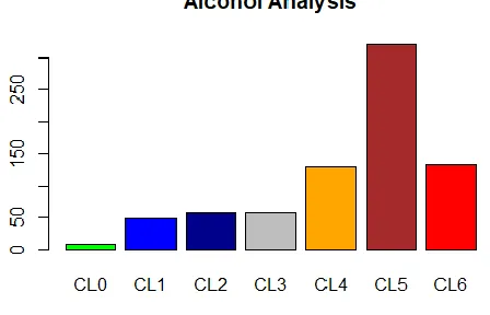
4.1 Naïve Bayes Classification Results
Fig (a): Analysis of consumption of Alcohol
The above figure represents the individuals Alcohol consumption levels based on their personality measurements using Naïve Bayes Classification. We can observe high result at CL5 which represents most of the users use it weekly.
Fig (b): Analysis of Benzos consumption
Equations
In this we can depict that highest result obtained at CL0. It represents most of the individuals never used this drug.
Fig (c): Analysis of Amphet Consumption
From this figure we can say that Amphet consumption levels at high at CL0 and CL6. These results are obtained using Naïve Bayes Classification.
Fig (d): Analysis of Amyl Consumption
4.2 Random Forest Results
a. Mean Decrease Gini: It is nothing but the total decrease in the impurity of the node that is averaged across all the trees generated for the forest.
b. Error Rate: The error rate of the resultant forest depends on two factors:
Correlation between the forests. If the correlation increases then error rate will also be increased.
Strength of every tree in the result.
A tree which has low error rate can be called as strongest classifier [2].
Table (a): Analysis of Alcohol
Attribute Mean Decrease Gini
ID 182.67610
Age 70.63748
Gender 29.90433
Education 81.36844
Country 46.78310
Ethnicity 28.58798
N-score 152.00684
E-score 142.77186
O-score 142.34055
A-score 142.45418
C-score 143.82962
Impulsive 97.28045
SS 107.74066
The above table represents the Mean Decrease Gini of the attributes based on Alcohol using random Forest.
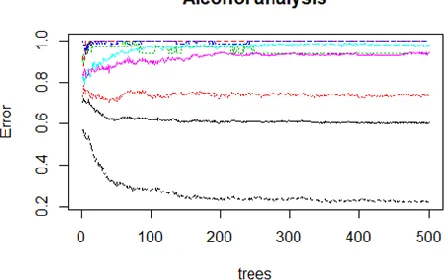
Fig (a): Analysis of Alcohol Consumption
The following figure depicts the analysis of alcohol consumption of the individuals.
Table (b): Analysis of Benzos
The following table represents the Mean Decrease Gini of the Benzos based on the attribute values using Random Forest.
Attribute Mean Decrease Gini
ID 159.52617
Age 68.98095
Gender 30.50798
Education 80.73338
Country 76.00160
Ethnicity 21.72528
Nscore 142.18732
Escore 124.59603
Oscore 126.70714
Ascore 122.87117
Cscore 126.74721
Impulsive 89.37260
SS 95.48849
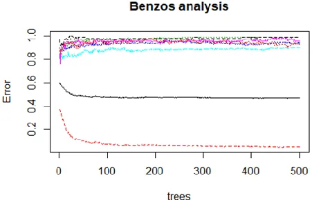
3474
The above figure depicts the error rate of the Benzos consumption analysis using random forest.
Table (c): Amphet Analysis
Attribute Mean Decrease Gini
ID 165.78455
Age 76.14502
Gender 30.07906
Education 82.51868
Country 70.39216
Ethnicity 19.23274
Nscore 128.66425
Escore 123.02513
Oscore 132.81690
Ascore 120.97324
Cscore 127.89709
Impulsive 90.97641
SS 111.78413
The above table represents the Mean Decrease Gini of the Amphet drug based on the attribute values using Random Forest algorithm.
Fig (c): Analysis of Amphet Consumption
The above figure depicts the error rate of Amphet Drug using Random Forest.
Table (d): Amyl Analysis
Attribute Mean Decrease Gini
ID 126.69576
Age 58.86520
Gender 21.23521
Education 59.44901
Country 47.47893
Ethnicity 12.31995
Nscore 92.02331
Escore 87.30788
Oscore 89.75799
Ascore 88.39786
Cscore 94.80778
Impulsive 65.60370
SS 75.32144
Based on the Attributes Mean Decrease Gini of Amyl can be depicted using Random Forest.
The above figure gives the error rate of the trees generated by the Random Forest. In the similar we can use this algorithm for the other drugs too.
4
CONCLUSION
Drug consumption risk analysis is done successfully with the two algorithms Naïve Bayes algorithm and Random forest. We got the accurate result. With the two classification algorithms we have drawn some important conclusions. Whenever we have values which are independent of the other features we can use Naïve Bayes classifier and when it comes to random forest it will be helpful when we have huge amount of data. The data set we have used can also be classified using Support Vector Machine (SVM), but it gives more accuracy when we have only two class labels. Here in this project we have seven class labels. For that we need Multi-Class Support Vector Machine [6]. It improves complexity. In the future we can get less complexity as many of the data scientists are currently working on it. Thus this project have a scope in future too as the data set is huge in volume. Moreover without any testing based on these scores we can know the consumption level of a person and suggest the remedies without any blood samples. Thus it will be helpful in medical field.
REFERENCES
[1] McGraw Hill - Machine Learning – Tom M Mitchell.
[2] ―The Five Factor Model of personality and evaluation of
drug consumption risk‖- IEEE paper.
[3] Amanpreet Singh , Narina Thakur and Akashanka Sharma, ―A Review of Supervised Learning Algorithms‖- IEEE .
[4] Veena N Jokhakar and S.V. Patel, ― A Random Forest
Based Machine Learning Approach For Mild Steel Effect Diagnosis‖- IEEE International Conference on Computational Intelligence and Computing Research (ICCIC).
[5] Hiroki Nakahara, Akira Janguji, Tomonoro Fujii and Simpei Sato, ―An Acceleration of a Random Forest Classification using Altera SDK for Open CL‖ 2016
Media Technology and Information Processing (ICCWAMTIP).
[7] Jakobwitz S, Egan V, The dark triad and normal personality traits,Personality and Individual Differences. 2006; 40(2):331–339.
[8] Venubabu Rachapudi and Golagani Lavanya Devi, ―Feature Selection for Histopathological Image Classification using levy Flight Salp Swarm Optimizer‖, Recent Patents on Computer Science (2019) 12: 329. https://doi.org/10.2174/2213275912666181210165129
[9] Veubabu Rachapudi,, Varikuti, V., Anubrolu, J., Geethika, C.R.,‖A comparative analysis of classification algorithms for fetal growth‖,Journal of Advanced Research in Dynamical and Control Systems, vol.9, pp. 592- 600,2017.
[10] Rachapudi, V., Lavanya Devi, G., Sai Chaitanya, N.,‖ A
nuclei segmentation method based on butterfly algorithm for h&e stained images‖, International Journal of Engineering and Advanced Technology,8(4), pp. 860-864,2019.
[11] Rachapudi, V., Vaddi, S.S., Karumuri, R.R., Sripurapu, S.,‖ Heart disease prediction using machine learning algorithms‖, International Journal of Recent Technology and Engineering,7(5), pp. 805-809,2019.
[12] Rachapudi, V., Venkata Suryanarayana, S., Subha Mastan Rao, T.,‖ Auto-encoder based K-means clustering algorithm‖, International Journal of Innovative Technology and Exploring Engineering,8(5), pp. 1223-1226,2019.