A COMPARATIVE STUDY OF REDUCED ORDER MODELLING USING STABILITY EQUATION

(1)

A COMPARATIVE STUDY OF REDUCED

ORDER MODELLING USING STABILITY EQUATION

Amir Khan

1

, Rajesh Bhatt

2

1,2

Department of Electronics Engineering, Rajasthan Technical University, Kota, (India)

ABSTRACT

The higher order systems (HOS) are generally costly and tedious for the analysis purpose. Also, the exact

analysis of HOS is very much complex for computation and synthesis. Hence, certain simplification procedures

based on practical model consideration or using the mathematical computation techniques are widely used to

get lower order systems (LOS) in place of original HOS. The analysis of LOS is easier and faster. The present

work deals with a simple mathematical method known as stability equation in order to obtain LOS. Results

obtained from stability equation have been compared with original HOS and also with the other lower order

systems already available in the literature. Time response specifications such as: rise time, settling time, peak

and peak time have also been compared for HOS & LOS. A comparative study of ISE has also been carried out

in the present work for HOS and LOS.

Keywords:

HOS, ISE, LOS, SISO, Stability Equation.

I

INTRODUCTION

Nowadays, all industries are becoming much complex to perform tasks because of increment in consumers and technologies. Power and control industries have also become the necessities in order to build a system which gives the most economical and appropriate results with least amount of cost. The higher order systems are generally very common in these industries which are much complicated, time consuming for analyst and costly for the synthesis.

Hence, simplification procedures based on either biological approaches or by using any mathematical algorithms are required to reduce a HOS into its equivalent LOS without excluding original HOS‟s characteristics in reduced LOS. Such techniques for obtaining lower order models from original HOS are known as Model order reduction (MOR) techniques [1-5]. There are various MOR techniques available in the literature to reduce any higher order system into its lower order system [6-9]. In the present work, an algorithm based on stability equation has been used to simplify the HOS. The results obtained from stability equation are comparable in performance with the other existing methods already available in the literature. The method gives better results in comparison to other existing methods, as shown in numerical examples. It has been observed that the stability of original HOS is preserved in its LOS.

(2)

reduction in present work, i.e. stability equation has been explained in section 3. Two numerical examples elaborating the suggested stability equation method have been given in section 4. Further, the conclusions obtained from the present carried out comparative study have been given in section 5 followed by the references.

II STATEMENT OF PROBLEM

Consider the following SISO higher order system of order „n‟:

1 0 0 ( )    



n i i i n i i i b s G s a s (1)

where, ai and bi are constants for i=1, 2…n.

The important requirement of any reduced order model is that it should contain all the basic important features of the original HOS [6]. If „r‟ represents the order of LOS which is lesser than „n‟, then, the reduced LOS of the system in (1) can be given as:

1 0 0 ( )    



r j j j r j j j d s R s c s (2)

where, cj and dj are unknown coefficients which have to be obtained by suggested stability equation method.

III STABILITY EQUATION METHOD

Assuming a higher order transfer function of the system as shown:

1

1 1 0

1

1 1 0

.... ( ) ....            m m m m n n n n

b s b s b s b G s

a s a s a s a (3)

( ) ( ) ( )

N s

G s

D s (4)

(4) is the symbolic representation of (3), The N(s) and D(s) are the numerator and the denominator of G(s) respectively. The order of D(s) is n and the order of N(s) is m such that n > m.

In order to get the reduced LOS, the steps of stability equation are[12] :-

The numerator and the denominator of (4) are divided in even and odd parts. If the even and odd parts are subscripted by „e’ and „o’ respectively, then the even and odd polynomials of numerator may be represented by Ne(s) and No(s) respectively. Similarly, the even and odd polynomials of denominator can be represented by De(s) and Do(s) respectively. Therefore, the system in (4) may be represented as:

( ) ( ) ( ) ( ) ( )    e o e o

N s N s G s

(3)

0,2,4 1,3,5 0,2,4 1,3,5 ( )       



m m i i i i i i n n i i i i i i

b s b s G s

a s a s

(6) 0,2,4 1,3,5 0,2,4 1,3,5 ( ) ( ) ( ) ( )       _         _    



m i e i i m i o i i n i e i i n i o i i N s b s N s b s D s a s D s a s

(7)

Roots of Ne(s) and No(s) are called zeros zi(s) and that of De(s) and Do(s) are called poles pi(s). In this method, a polynomial is reduced by successively discarding the less significant factors. By this method, the numerator and denominator are reduced and the ratio of reduced numerator and denominator gives the reduced order model. The denominator is separated as follows:

D s

( )



D

e

( )

s



D

o

( )

s

(8) where,

2 4

3 5

1 3 5

( ) ... ( ) ...           _{ } e o o

D s a a s a s D s a s a s a s

(9)

Then (9) can be written as follows:

1 2 2 2 1 2 1 2 1

( ) (1 )

     _      _ 



k e o i i k o i i s D s a

z s D s a s

p

(10)

where, k1 and k2 are integer parts of n/2 and (n-2)/2 respectively and z12 < p12 < z22 < p22… by discarding the

factors with larger magnitude of zi and pi, the reduced stability equations of required order r now becomes:

1 2 2 2 1 2 1 2 1

( ) (1 )

     _      _ 



r er o i i r or i i s D s a

z s D s a

p

(11)

where, r1 and r2 are the integer parts of r/2 and (r-1)/2, respectively. The reduced denominator of the system is

given as:

( ) ( ) ( )

r er or

D s D s D s (12) The numerator of the reduced system can be represented as:

N_r( )s N_er( )s N_or( )s (13) Therefore the complete system of the rth order reduced model can be given as in (14):

( ) ( ) ( ) ( ) ( )    er or er or N s N s R s

D s D s (14)

(4)

magnitudes and therefore poles and zeros with larger magnitudes are discarded. Thus, the ROS preserves the dominant performance of the original HOS.

IV NUMERICAL EXAMPLES

In this section, two numerical examples have been given to elaborate the suggested stability equation method. The performance index ISE known as integral square error in between the transient parts of HOS and LOS has also been calculated to measure the goodness of the LOS (i.e. smaller the ISE, the closer is R(s) to G(s)), which is given by:

I.S.E. = 2

0 [ ( ) ( ) ]







y t yr t dt (15)

where, y(t) and yr(t) are the unit step responses of original and reduced order systems.

4.1 Example-1

. Consider a SISO HOS of 4th order given by [13]:

3 2

4 4 3 2

7 24 24 ( )

10 35 50 24

  



   

s s s G s

s s s s

(16)

4.1.1 ROM using Stability Equation method

Reduction of numerator:

The numerator of (16) with its even and odd terms is given as: 3 2

( ) 7 24 24

N s s s s

3 2

24 7 24

 __ ____

odd even

s s s (17)

Step-1: Reduction of 3rd order numerator to a 1st order: 3 2

( ) 7 24 24

N s s s s

 

2 2

0.04167 0.29167

1 7

24 (1 ) 24 (1 )

24 24

 

 s  s   s

24s24 (18) Reduction of denominator:

The denominator of (16) with its even and odd terms is given as:

4 3 2

( ) 10 35 50 24

D s s s s s

4 2 3

35 24 10 50

_{}   _{}

even odd

s s s s (19)

Step-1: Reduction of 4th order denominator to a 2nd order:

 

2 2 2

0.0285 0.2

1 10

( ) 35 (1 ) 50 (1 ) 24

35 50

 

    

D s s s s s

2

35 50 24

 s  s (20) The 2nd order reduced model from (18) and (20) is given as:

2

2 2

2

( ) 24 24

( )

( ) 35 50 24



 

 

N s s R s

(5)

4.1.2 Comparison of Step and Frequency responses

In order to verify the applicability of the LOS from suggested stability equation method and reduced order models already available in the literature for the same HOS by the other researchers, the step and frequency responses have been compared, as shown in Figs. (1-4).

Fig.1. comparison of step responses of HOS (4

th

order) and LOS (2

nd

order).

Fig.2. comparison of frequency responses of HOS (4

th

Order) and LOS (2

nd

order)

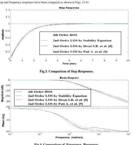
4.1.3 Comparison of Stability Equation with other Existing Methods [8, 9]

2nd order LOS of (16) obtained by Desai S.R. et al. [8] is:

2 2

0.7645 1.689 ( )

2.591 1.689

 

 

s G s

(6)

2nd order LOS of (16) obtained by Pati A. et al. [9] is:

2 2

24.0096 ( )

27.0096 24.0096

 

 

s G s

s s

(23)

Step and frequency responses have been compared as shown in Figs. (3-4):

Fig.3. Comparison of Step Responses.

Fig.4. Comparison of Frequency Responses.

Table 1. Comparison of Transient Response Parameters

System Rise Time(sec) Settling Time(sec) Peak Peak Time(sec)

Original HOS (4th Order) 2.2602 3.9307 0.9991 6.9770

LOS (2nd Order) 2.3008 3.3764 1.0125 5.2144

Desai SR et al. [8] 2.2616 3.8443 1.0000 9.6778

(7)

Table 2. Comparison of Reduced Models

Method Reduced Models ISE

Stability Equation method

2

24 24 35 50 24



 

s s s

0.0035

Desai SR et al. [8]

2 0.7645 1.689 2.591 1.689    s s s 0.7417

Pati A et al. [9]

2 24.0096 27.0096 24.0096    s s s 0.0011

4.2 Example-2.

Consider a SISO HOS of 4th order given by [12]:

3 2

4 4 3 2

28 496 1800 2400 ( )

2 36 204 360 240

s s s G s

s s s s

  



    (24)

4.2.1 ROM using Stability Equation method

reduction of numerator:

The numerator of (24) with its even and odd terms is given as:

3 2

( ) 28 496 1800 2400

N s  s  s  s

3 2

28s 1800s 496s 2400

    (25) Step-1: Reduction of 3rd order numerator to a 1st order:

 

2 2

0.0156 0.20667

28 496

( ) 1800 (1 ) 2400 (1 )

1800 2400

N s s s s

 

   

1800s 2400

  (26) Reduction of denominator:

The denominator of (24) with its even and odd terms is given as:

4 3 2

( ) 2 36 204 360 240

D s  s  s  s  s

4 2 3

2 204 240 36 360

even odd

s s s s

    

  (27)

Step-1: Reduction of 4thorder denominator to a 2ndorder:

 

2 2 2

0.0098 0.10

2 36

( ) 204 (1 ) 360 (1 ) 240

204 360

D s s s s s

 

    

2

204s 360s 240

   (28) The 2nd order reduced model from (26) and (28) is given as:

₂

2

1800 2400 ( )

204 360 240

s R s

s s

 

  (29)

4.2.2 Comparison of Step and Frequency responses

(8)

responses have been compared, as shown in Figs. (5-8).

Fig.5. comparison of step responses of HOS (4

th

order) and LOS (2

nd

order).

Fig.6. comparison of frequency responses of HOS (4

th

order) and LOS (2

nd

order).

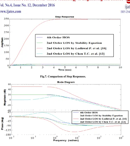
4.2.3 Comparison of Stability Equation with other Existing Methods [10, 12]

2nd order LOS of (24) obtained by Lodhwal P. et al. [10] is: ₂

2

14 410.256 ( )

1.785 1.19

 

 

s R s

s s (30)

2nd order LOS of (24) obtained by Chen T.C. et al. [12] is:

2 2

8.93 1.19 ( )

1.785 1.19

 

 

s R s

s s

(31)

(9)

Fig.7. Comparison of Step Responses.

Fig.8. Comparison of Frequency Responses.

Table 3. Comparison of Transient Response Parameters

System Rise Time(sec) Settling Time(sec) Peak Peak Time(sec)

Original HOS (4th Order) 1.6920 2.5514 10.0443 3.9460

LOS (2nd Order) 1.6150 4.3379 10.2711 3.4483

Lodhwal P et al. [10] 4.5602 8.1197 29.2387 16.2215

(10)

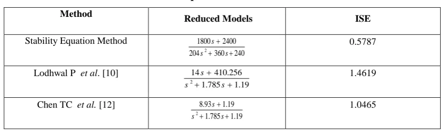
Table 4. Comparison of Reduced Models

Method

Reduced Models ISE

Stability Equation Method

2

1800 2400 204 360 240

s s s



 

0.5787

Lodhwal P et al. [10]

2

14 410.256 1.785 1.19

s s s



 

1.4619

Chen TC et al. [12]

2

8.93 1.19 1.785 1.19

s s s



 

1.0465

V CONCLUSIONS

The present work deals with the reduced order modelling of large scale SISO systems. The HOS have been reduced by stability equation method and the performance is compared with other order reduction methods already available in the literature. The transient response parameters such as; rise time, settling time, peak and peak time of both HOS and LOS have been compared. It has been observed that reduced order system obtained using stability equation is more appreciable as compared to the ROMs already available in the literature for the same HOS. The step and frequency responses of HOS and LOS have also been compared and it is found that response of LOS obtained by stability equation is effectively closer to the HOS.

REFERENCES

[1]. Davison E.J., “A method for simplifying linear dynamic systems”, IEEE Trans. Automat. Control, vol. AC-11, pp. 93-101, 1966.

[2]. Parmar G., Prasad R. and Mukherjee S., “Order Reduction of Linear Dynamic Systems using Stability Equation Method and GA”, International Journal of Electrical, Computer, Electronics and Communication Engineering, vol. 1, no. 2, 2007.

[3]. Hutton M. F. and Friedland B., “Routh approximations for reducing order of linear time invariant systems” IEEE, Jan 1975.

[4]. Gutman P.O., Mannerfelt C, Molander P., “Contributions to the model reduction problem”, IEEE Transactions on AutomaticControl. 1982; 27(2):454-455.

[5]. Lucas T., “Differentiation reduction method as a multipoint pade Approximant”, Electronics Letters. 1988; 24(1):60-61.

[6]. Lucas T., “A tabular approach to the stability equation method”. Journal of the Franklin Institute.1992; 329(1):171-180.

[7]. Krishnamurthy V., Seshadri V. , “Model reduction using the routh stability criterion”. Automatic Control, IEEE Transactions on.1978; 23(4):729-731.

[8]. Desai S.R., Prasad R., “Implementation of order reduction on tms320c54x Processor using genetic algorithm”, In: Emerging Research Areas and 2013 International Conference on Microelectronics, CommunicationsAnd Renewable Energy (AICERA/ICMiCR). 2013; 1-6.

(11)

Engineering. 2014;5(2014).

[10]. Lodhwal P., Jha S., “Performance comparison of different type of Reduced order modeling methods”, In: Third International Conference On Advanced Computing and Communication Technologies (ACCT,

'13'). 2013; 95-100.

[11]. Desai S.R., Prasad R., “A new approach to order reduction using Stability equation and big bang big crunch optimization”, Systems Science & Control Engineering. 2013; 1(1):20-27.

[12]. Chen T.C., Chang C.Y., Han K.W., “Model reduction using the stability-equation method and the continued-fraction method”, InternationalJournal of Control. 1980; 32(1):81-94.