T E C H N I C A L N O T E
An Optimization Algorithm for Exponential Curve Model
of Single Pile Bearing Capacity
Hongmei Ma.Cheng Peng.Jinying Gan.Yonghong Deng
Received: 27 May 2019 / Accepted: 11 December 2020 The Author(s) 2021
Abstract The ultimate bearing capacity of single pile is very important to engineering safety, so correctly predicting its value becomes an important part of engineering safety. Based on the traditional exponential curve model, a parameter optimization algorithm of the exponential curve model of single pile bearing capacity, which combines the golden section method and the linear least square method, is proposed. In order to verify the reliability of the proposed optimization algorithm, the measured data of the building engineering in the literature were opti-mized and calculated. Through comparison, it is found that the optimization algorithm is closer to the measured value than the traditional exponential curve model algorithm, which can better guide the engi-neering practice, and verify the effectiveness and superiority of the proposed parameter optimization method.
Keywords Ultimate bearing capacityExponential curve modelGolden section searchLinear least squares
1 Introduction
The bearing capacity of piles can be determined based on conventional semi-empirical equations. In this regard, the Meyerhof equation is still well-respected. In addition, there are some simple correlations between the bearing capacity of piles and in-situ tests (like cone penetration test, CPT or standard penetra-tion test, SPT); however, some studies suggest that the aforementioned correlations overestimate the bearing capacity. Furthermore, some other studies recommend the use of dynamic equations, which are based on the pile and hammer properties, to estimate the bearing capacity of piles; however, as stated by Milad et al. (Milad et al. 2015), there are many assumption and simplification in estimating the bearing capacity using the aforementioned equations. (Ehsan Momeni et al.
2020; HAN Jiwei et al.2020).
Reasonable and correct prediction of vertical ultimate bearing capacity of single pile is the most important safety premise in pile foundation engineer-ing. The existing models are widely used because of the advantages of exponential curve model. In the use of exponential curve model, the reasonable solution of its unknown parameters is the key problem for prediction. The existing methods mainly use the traditional intelligent optimization algorithm or gra-dient optimization algorithm to complete this task (Peng et al.2010). In engineering, we find that we can explore more optimized algorithm, so we propose an optimization algorithm combining golden section H. Ma (&)C. PengJ. GanY. Deng
School of Electronic and Information Engineering, North China University of Science and Technology,
Yanjiao Town, East of Beijing 065201, China e-mail: [email protected]
method and linear least square algorithm. (Julong et al.
2012; Xing et al.2016).
2 Problem Description
In order to predict the ultimate bearing capacity, the exponential curve model is used in this paper (Deling
2003; Nehdi2015). Q¼Qu 1AeBs
; ð1Þ
In it, S represents stable settlement (mm), Q is the test load corresponding to s ( kN), Unknown param-eters in the model are A,B and theoretical ultimate bearing capacityQu(kN) at s??
It is assumed that the stable settlement ofngroupSi
(i= 1,2,… n) and its corresponding test load Qi
(i = 1,2,…n) are obtained by test pile test, then the unknown parameter can be obtained by optimizing that nonlinear least squares cost function (Jiang et al.
2016). minJðA;B;QuÞ ¼ Xn i¼1 QiQu 1AeBsi 2 ð2Þ
3 Exponential Curve Fitting Method 3.1 Separable Least Squares Problem
Genetic algorithm may also be used Genetic algo-rithms can also be used. The nonlinear least squares cost function defined by (2) can be solved by standard nonlinear least squares optimization method, such as Gauss–Newton method or Marquardt method. Genetic algorithm, differential evolution and other intelligent optimization methods can also be used to solve this problem. However (Yan et al. 2015; Zhang et al.
2015), the above methods do not take into account the characteristics of the unknown parameters in the model (1). For the convenience of analysis, order:
A1¼QuA; ð3Þ
Then the formula (1) and (2) are converted into:
Q¼QuA1eBs; ð4Þ minJðA;B;QuÞ ¼ Xn i¼1 QiQuA1eBsi 2 ð5Þ And then it’s easy to know, If B is known quan-tity, The nonlinear least squares problem defined by (5) will be simplified to a linear least squares problem. In addition, if let: N¼ Q1 Q2 .. . Qn 2 6 6 6 4 3 7 7 7 5;. . .M¼ 1 eBs1 1 eBs2 .. . .. . 1 eBsn 2 6 6 4 3 7 7 5; ð6Þ
Another two unknown parameters in the formula (4):
Qu
A1
¼MTM1MTN ð7Þ
Through the analysis above, we can see that the nonlinear least squares problem defined by (5) is variable separable. For this kind of nonlinear least squares problem, the nonlinear parameters and linear parameters can be divided into two groups estimated separately. The nonlinear parameter B can be esti-mated by nonlinear optimization techniques. In this paper, golden section method as a commonly used method in univariate optimization problems is used. Quand A1 are linear parameters, them can be obtained
through formula (7). 3.2 Golden Section Method
The main idea of the golden section method is to find the optimal solution by narrowing the area of the optimal solution step by step. In the process of optimization, only the value of the finite cost function needs to be calculated. To calculate the objective function value required by the golden section method (Arnau et al.2012), let B take a particular value, First, the linear parametersQuand A1 corresponding to B is
calculated by formula (7), the objective function J corresponding to B, Qu and A1 is calculated by the
formula (5).
For one dimension optimization problem: minfðxÞ; x2 ½a;b
Order constant h= 0.618, the first step in the Golden Section, let x ¼aþ ð1hÞ ðbaÞ,
The second step in the Golden Section is to compare the size offðx1Þandfðx2Þ. Iffðx1Þ fðx2Þ,
the interval of the optimal solution is reduced to [a, x2],
this situation orderb¼x2, the interval of the optimal
solution can still be recorded as [a, b], at the same time, let x2¼x1, fðx2Þ ¼fðx1Þ,
x1¼aþ ð1hÞ ðbaÞ, calculate the value of
fðx1Þ; If fðx1Þ ¼fðx2Þ, the interval of the optimal
solution is reduced to½x1;b, at this point,a¼x1, the
interval of the optimal solution can still be recorded as ½a;b, at the same time, let x2¼x1, fðx2Þ ¼fðx1Þ,
x1¼aþh ðbaÞ, then calculatefðx2Þ.
The second step is repeated several times until the length of the interval½a;bis less than a predetermined constante,so that the optimal solutionxb¼ ðaþbÞ=2
can be obtained.
After each iteration, the golden section reduces the length of the search interval to h times that of the previous one (Xue et al.2015; Sun et al.2015). 3.3 Algorithm Flow
In summary, the golden section-least square procedure of estimating the unknown parameters a\b and qu in the exponential curve model defined by the formula (1) is as follows:
(1) Sets the constant erequired to end the golden section search, order constant h¼0:618; Sets the range of values of the parameter B½a;b. (2) Let B1 ¼aþ ð1hÞ ðbaÞ, the
corre-sponding objective functionJ1is calculated by
the formula (5); Let B2¼aþbB1, the
corresponding objective function J2 is
calcu-lated by the formula (5).
(3) Compare the size ofJ1 andJ2. IfJ1J2, order
b¼B2, B2 ¼B1, J2¼J1,
B1 ¼aþ ð1hÞ ðbaÞ, J1 is calculated
by the formula (5); Otherwise, order a¼B1,
B1 ¼B2, J1¼J2, B2¼aþh ðbaÞ, J2 is
calculated by the formula (5).
(4) Ifbae, return to the step (3); Otherwise, let the optimal solutionB¼ ðaþbÞ=2, the linear parameter and corresponding to B* are calcu-lated by formula(3), (4), the objective function J* corresponding to, and can be calculated by formula (5). LetA*=A* 1/Q* u, to find out the
optimal solutionB*,A*,Q* u and the optimal objective function J*.
4 Example of Practical Calculation
To verify the performance of the above algorithm, Taking into account the static load test data of Wuhan Power Market Building provided by reference (Deling
2003), Set the constante¼1104 required by the
golden section method, Set the range of parameter B½0;20(Fig.1).
According to the static load test data of Wuhan power market building provided by literature (Deling
2003), the predicted value is calculated by golden section least square method according to the algorithm flow of 3.3, and compared with the prediction data in literature (Deling2003) and Literature. The detailed results are shown in Table1.
The model fitting accuracy in Table1is defined as: w¼ ffiffiffiffiffiffiffiffiffiffiffiffiffiffiffiffiffiffiffiffiffiffiffiffiffiffiffiffiffiffiffiffiffiffiffiffiffiffiffiffiffiffiffiffiffiffiffiffiffiffiffiffiffiffiffiffiffiffiffiffiffiffiffiffiffiffiffiffiffiffiffiffiffi 1X n i¼1 QiQmi ð Þ2 , Xn i¼1 QiQ 2 v u u t
whereQmi corresponds toQi, The load value calculated
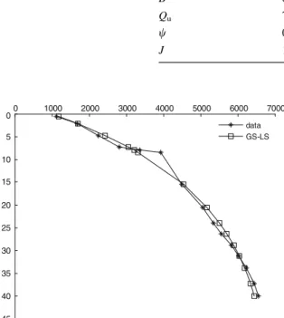
by the model is KN, Q is the average value of measured loadQi(i = 1,2,…n) (Fig.2and Table2).
5 Conclusion
According to the traditional exponential model curve fitting method, an exponential model curve fitting optimization algorithm is proposed, and its theoretical prediction of the ultimate load of a single pile is deduced. The calculation results for typical problems show that this method has the advantages of small amount of calculation and high model accuracy. From the data, the fitting precision of curve fitting opti-mization algorithm of exponential model is higher than that of traditional method. Through comparison, it can be seen that the exponential model curve fitting optimization algorithm is more safe and reliable to predict the limit load value, and can meet the need of high precision in prediction or design.
Table 1 The optimal solutions obtained by different methods and their comparison
Calculation results Literature (Deling
2003)
Literature This paper
A 0.9470 0.8600 0.8607 B 0.0650 0.0552 0.0568 Qu 7000 7151 7070 w 0.9855 0.9932 0.9934 J 1.349106 6.249105 5.969105 0 1000 2000 3000 4000 5000 6000 7000 0 5 10 15 20 25 30 35 40 45 data GS-LS
Fig. 2 A comparison figure between the golden section-the least squares solution and the measured values
Table 2 Comparison
table of different algorithm fitting results
Settle-Ments/mm LoadQ=kN
measured value Literature (Deling
2003)
Literature this paper
0.58 1123 616 1195 1182 2.20 1685 1254 1704 1699 4.75 2246 2132 2419 2423 7.31 2808 2878 3043 3052 8.02 3370 3064 3201 3211 8.51 3931 3187 3306 3317 15.43 4493 4569 4526 4536 20.56 5054 5258 5173 5177 23.98 5346 5605 5513 5511 26.33 5553 5803 5713 5706 28.85 5824 5984 5899 5888 31.24 6032 6130 6054 6038 33.91 6240 6269 6204 6183 37.35 6448 6415 6368 6340 40.12 6556 6511 6479 6447
Acknowledgements The project was supported by the Central University Basic Research Operating Funding Project (3142012036, 3142012039).
Open Access This article is licensed under a Creative Com-mons Attribution 4.0 International License, which permits use, sharing, adaptation, distribution and reproduction in any med-ium or format, as long as you give appropriate credit to the original author(s) and the source, provide a link to the Creative Commons licence, and indicate if changes were made. The images or other third party material in this article are included in the article’s Creative Commons licence, unless indicated otherwise in a credit line to the material. If material is not included in the article’s Creative Commons licence and your intended use is not permitted by statutory regulation or exceeds the permitted use, you will need to obtain permission directly from the copyright holder. To view a copy of this licence, visit
http://creativecommons.org/licenses/by/4.0/.
References
Arnau O, Molins C (2012) Three dimensional structural response of segmental tunnel linings. Eng Struct 44(6):210–221
Cheng P, Yong W (2010) Frequency domain identification of vibration system stability model. Vib shock 29(3):118–120 Deling Q (2003) Interaction mechanism between soil and pile with variable section[M]. HeFei University of Technology Press, HeFei, pp 58–61
Jiang H, Cao Q, Liu A et al (2016) Flexural behavior of precast concrete segmental beams with hybrid tendons and dry joints. Constr Build Mater 110:1–7
Jiwei H, Xiaoming L, Yuehong Y et al (2020) Study on the horizontal bearing capacity of single pile foundation con-sidering spatial variability of soil strength. Hydr Sci Eng
Julong S, Xiangke W, Xiaohui F (2012) optimization method [M]. Xian Electronic Sience & Technology University Press, XiAn
Milad F, Kamal T, Nader H, Erman OE (2015) New method for predicting the ultimate bearing capacity of driven piles by using Flap number. KSCE J Civ Eng 19:611–620 Momeni E, Dowlatshahi MB, Omidinasab F et al (2020)
Gaussian process regression technique to estimate the pile bearing capacity. Arab J Sci Eng 45:8255–8267
Nehdi ML, Abbas S, Soliman AM (2015) Exploratory study of ultra-high performance fiber reinforced concrete tunnel lining segments with varying steel fiber lengths and dosa-ges. Eng Struct 101:733–742
Sun LH, Wu HY, Yang BS et al (2015) Support failure of a high-stress soft-rock roadway in deep coal mine and the equal-ized yielding support technology: a case study. Int J Coal Sci Technol 2(4):279–286
Xing Wanli Yu, Yinquan JH et al (2016) Experimental study on large-span steel arch in Shijiazhuang railway station. Build Struct 19:21–25
Xue JH, Wang HP, Zhou W et al (2015) Experimental research on overlying strata movement and fracture evolution in pillarless stress-relief mining. Int J Coal Sci Technol 2(1):38–45
Yan ZG, Shen Y, Zhu HH et al (2015) Experimental investi-gation of reinforced concrete and hybrid fibre reinforced concrete shield tunnel segments subjected to elevated temperature. Fire Saf J 71(3):86–99
Zhang CH, Wang LG, Du JH et al (2015) Numerical modelling rock deformation subject to nitrogen cooling to study permeability evolution. Int J Coal Sci Technol 2(4):1–6
Publisher’s Note Springer Nature remains neutral with regard to jurisdictional claims in published maps and institutional affiliations.