Environmental Conservation as an Engine for Economic Growth:
Testing the Validity of Environmental Kuznets Curve on Carbon Emissions for Kenya1 By
Mercyline W. Kamande, Department of Economics, University of Dares Salaam,
P.O. Box 35045, Dares Salaam; Mobile Phone: +255784350286; Email: [email protected]
Abstract
Environmental Kuznets Curve hypothesis postulates an inverted U-shaped relationship between Carbon dioxide emissions and per capita income. However, the experiences of many countries show that economic growth is causing an increase in resource use and pollution more than it is a solution to environmental problems. The consequences of neglecting environmental conservation can be drastic. This study investigates the role of environmental conservation as an engine for economic growth in Kenya by exploring the relevance of the Environmental Kuznets Curve. Using time series data from World Development Indicators for Kenya for the years 1960 to 2006, a quadratic Environmental Kuznets Curve between per capita carbon emissions and per capita GDP is estimated.The study finds no evidence for the inverted-U relationship but rather a cyclical relationship is observed. Given these findings, the responsibility of environmental conservation cannot be passively left to economic growth but rather deliberate efforts must be made to ensure a clean environment. This is possible by pursuing a vigorous environmental policy alongside economic development policy.
Key Words: Environmental Kuznets Curve, Environmental Conservation Carbon Emissions
1 This paper is an extract from my PhD Thesis (work in progress) entitled ‘
The Economics of Clean Production in Kenyan Manufacturing Sector ’. I am indebted to my supervisors, Dr.G. Kahyarara and Dr.
1.0: Introduction
Economic growth is one of the principle objectives in the macroeconomic policy arena. It is seen as the only vehicle out of poverty which is a great challenge in most developing countries. For a country to achieve the desired level of economic growth, it must have the necessary resources such as energy and other natural resources. In order to make economic development sustainable, resources must be utilized in such a way that there is enough for the present generation as well as the future generation. It is therefore paramount to ensure the conservation of the environment that holds these vital natural resources.
While both environmental conservation and economic growth are important for human existence, there is a looming debate as to whether they can be achieved simultaneously (see Bennett et. al., 2008; Hediger, 2006). The question is how much of the environmental resources should be exploited in order to ensure rapid economic growth. Environmental degradation has been a source of numerous challenges some of which undermine the macroeconomic objectives of economic growth and poverty alleviation. The climatic change crisis which is responsible for global warming threatens the very existence of humanity and availability of enough natural resources to ensure sustainability of economic growth. The experience of newly industrialized countries such as Bangkok and Beijing show that they are more polluted today than they were twenty to thirty years ago. On the contrary, cities in older industrial countries such as New York, Tokyo and London are cleaner than they were twenty to thirty years ago. This apparent paradox raises the question of whether higher income levels result in a better or worse environment. (Encycropedia.com, 2008).
The paradox can best be understood by looking at two distinct schools of thought. Proponents of smart growth argue that economic development should be integrated with the community’s quality-of-life by preserving the natural environment (see MAPC, 2010). This implies that to ensure sustainable economic growth, environmental resources must be used responsibly because most of them are non-renewable and some of the consequences of environmental degradation are irreversible. Another school of thought is the ‘going-for-growth’ perspective which emphasizes on achieving faster economic growth rather than on forming environmentally friendly policies because economic growth is perceived to be able to achieve both economic and environmental goals, whereas implementing environmental policies may impede economic growth. (Webber and Allen, 2004). This implies that countries should be allowed to economically grow out of environmentally damaging activity. The proponents of this policy further argue that it is possible to allow initial environmental degradation to accelerate economic growth such that the realized income will be used for environmental management.
The correct balance between environmental protection and economic growth continues to be debated. Both of the opposing views present important arguments. However, having either extreme, which calls for a tradeoff scenario between economic activity and conservation, is an inadequate solution. On one hand we clearly must not abandon the preservation of the environment as doing so would jeopardize the vitality of our world. Unfortunately, the alternative is equally disagreeable as we cannot merely forgo economic development. Sawmill (1993) suggests that we cannot talk of choosing between them because the environment cannot be viewed as a separate entity that exists independent of human activity. The fact is that the environment undergirds everything we do; provides the essentials of life such as food, water, air,
and natural resources. The more we destroy the environment, the less able it is to support us. A more suitable policy option is one that supports both enhanced livelihood strategies for the poor and more sustainable management of environmental resources, the win-win scenario (Scherr, 1999)
.
This study seeks to validate the second argument that countries should be allowed to economically grow out of environmentally damaging activities. A well-known hypothesis that provides support for a policy that emphasizes economic growth at the expense of environmental protection is the environmental Kuznets curve (referred to also as EKC hypothesis interchangeably). The main objective of this study is to investigate the relationship between environmental conservation and economic growth by exploring the relevance of the Environmental Kuznets Curve hypothesis. This hypothesis postulates that countries in their development process will see their levels of environmental degradation increase until some income threshold is met and then afterwards decrease which suggests an inverted U-shaped relationship between different pollutants and per capita income. If this relationship holds, then economic growth could be a powerful way for improving environmental quality in developing countries in that it will be possible for countries to economically grow out of environmentally damaging activities. If the relationship does not hold, environmental conservation initiative could be a useful instrument of economic policy to ensure sustainable development. Specifically the study tests the validity of the Environmental Kuznets Curve hypothesis for carbon dioxide emissions using time series data from World Development Indicators for Kenya for the years 1960 to 2006.
This is best addressed by answering several questions which include: 1. Is the Environmental Kuznets Curve hypothesis true for Kenya? 2. Is it useful as an instrument for economic policy?
3. What is the future path of carbon emissions?
An understanding of this relationship is important in the policy arena because any policy that is aimed to catalyze economic development should also not leave some of the population, especially the vulnerable poor, worse-off. A more integrated approach that enables economic growth to support and reinforce environmental sustainability is more appropriate, which is a stride towards sustainable development. Investigating any possible pre-conditions for Environmental Kuznets Curve is important because it will cushion the government from embracing the hypothesis blindly without considering what is necessary for it to work. This will inform the policy makers what is necessary for the hypothesis to be a win-win situation between environmental conservation and economic growth. It is also expected to add knowledge to the ongoing debate of environmental sustainability for sustainable development.
After this introduction, the next section 2.0 of this chapter reviews the literature on Environmental Kuznets Curve Hypothesis. Section 3.0 discusses the methodology, section 4.0 discuses the empirical findings while section 5.0 presents the conclusion and recommendations
2.0: Review of Related Literature
2.1: Conceptual Literature Review
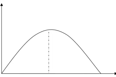
The concept of Environmental Kuznets Curve originates from the work of Simon Kuznets (1955) who hypothesized the Kuznets curve as an inverted U-shaped relationship between actual income per person and income inequality. Kuznets (1955) observed that inequality tends to increase during the early stages of growth and to decrease later on, describing an inverted-U shaped relationship between per capita income (on the horizontal axis) and income inequality (on the vertical axis). In the 1990s, beginning with the work of G. M. Grossman and A. B. Krueger (1991), the Kuznets curve took on a new face becoming an instrument for describing the relationship between the levels of environmental quality and per capita income. The term Environmental Kuznets Curve was coined by Panayotou (1993) given its resemblance to Kuznets’ hypothesis. Graphically, the relationship is represented as in figure 1 below.
Figure 1: Environmental Kuznets Curve
The environmental Kuznets curve hypothesis represents a long-term relationship between environmental impact which is defined as the level of concentration of pollution or flow of emissions and depletion of resources, and economic growth. As income of an economy grows
over time, the emission level grows first, then reaches a peak at Y* and then starts declining. Point Y* is known as the threshold level of income at turning point.
Apart from the original representation of the inverted U-shaped environmental Kuznets curve, other functional forms have been confirmed. A linear relationship between GDP and carbon emissions was confirmed by Shafik and Bandyopadhyay (1992) and Shafik (1994). Cole, M.A.
et al. (1997) suggest that using a linear functional form for predictions as opposed to the quadratic form is more appropriate since even the countries with highest incomes are still on the upward sloping part of the quadratic function. An N-shaped environmental Kuznets curve has also been confirmed (see de Bruyn et al., 1998). Moomaw and Unruh (1997) suggest that an N-shaped curve is more the result of polynomial curve fitting than a reflection of any underlying structural relation. In addition, if an N-shaped pattern is obtained, the second turning point usually occurs at relatively high per capita income levels reached only by very few countries. A U-shaped relationship has also been confirmed in Nigeria (see Olusegan, 2009)
Theoretically, the inverted U-shape is explainable from the linear stage theory of economic development where all societies are seen to develop through five stages: The traditional society, preconditions for take-off stage, the take-off stage, the drive to maturity stage and the stage of higher massive consumption (Rostow, 1960). The first two stages represent a clean agrarian economy with no pressure on the environment. At the take-off stage, the process of industrialization sets in. Rapid growth inevitably results in greater use of natural resources and emission of pollutants, which in turn puts more pressure on environment. As economic development accelerates towards maturity, the rate of resource depletion begins to exceed the
rate of resource regeneration, and waste generation increases in quantity and toxicity. At higher levels of development, the structural change towards information-intensive industries and services, coupled with increased environmental awareness, enforcement of environmental regulations, better technology and higher environmental expenditures, results in leveling off and gradual decline of environmental degradation (Pasche, 2002). The developed world is seen to have gone through such a development pattern and it is argued that developing countries must also pass through the same phases in order to achieve economic growth. Therefore, if they are forced to adhere to strict environmental regulations at an early stage of development, this will constitute a comparative disadvantage compared to the already developed countries.
The sustainable development trajectory can also be explained from the perspective of workers’ preferences. At the initial stages of development, the major challenge is poverty; people are too poor to care about the environmental consequences of growth. They are more interested in jobs and income than clean air and water (Dasgupta et al., 2002). At a later stage of industrialization, as income rises, people value the environment more and regulatory institutions become more effective. Hence beyond the turning point, pollution level declines improving the environmental quality. From this view, a high-income level can help to reduce environmental damage is by altering the demand for environmental quality, which is seen as an “income effect where individuals place environmental quality above additional economic growth. According to the EKC hypothesis, changes to evolving economies and the individual preference for environmental quality combine to determine the income threshold. From the foregoing, it is important to explore how an environmental Kuznets curve for Kenya would look like..
2.2: Empirical Literature Review
There are two strands of empirical literature on environmental Kuznets curve hypothesis. The first strand uses panel data in a cross-country setting to investigate the relationship between economic growth and environmental quality dating back to the 1990s beginning with the work of Grossman and Krueger (1991). These cross-country studies have led to mixed results concerning the existence of an Environmental Kuznets Curve with some supporting the hypothesis predict a U shaped Environmental Kuznets Curve (see Selden and Song (1994), Grossman and Kruger (1991), Grossman and Kruger (1995), Hettige et al. (2000), among others). Other studies have reported a linear relationship (see (Shafik and Bandyopadhyay, 1992 and Hettegi et al., 1992) while others have found an N shaped function (see de Bruyn et al., 1998; Friedl and Getzner, 2003 among others).
The second strand is a historical approach that makes use of time series data for single countries. Most of the time series studies are for developing countries (for instance Vincent, 1997) with only a few addressing industrialized countries (see Friedl and Getzner, 2003). Lindmark (2002) argues that historical studies of individual countries offer an advantage over cross-section approaches in bringing the analyses closer to the dynamics that cause the environmental Kuznets curve pattern. Further, Stern et al. (1996) argues that time-series data of a single country may be able to account for historic experience such as environmental policy, development of trade relations, and exogenous shocks such as the oil crisis. The next section explores cross-country literature on the relationship between economic growth and environmental quality.
2.2.1: Cross-Country Studies
Grossman and Krueger (1991), while investigating the environmental impacts of North American Free Trade Agreement (NAFTA) based on the GEMS dataset, use a cross-section sample of comparable measures of air pollutants for urban areas in 42 countries to explore the relationship between air quality and economic growth. They find that for SO2 and dark matter
(fine smoke) concentration increase with per capita GDP at low levels of national income but decrease with GDP at higher levels of income, depicting an inverted u-shaped relationship with the turning points for both SO2 and dark matter are at around $4000-5000. However, for
suspended particles (SPM), the relationship is monotonically decreasing (see also Grossman and Krueger,1995).
Shafik and Bandyopadhyay’s (1992) estimate Environmental Kuznets Curves for ten different indicators using three different functional forms. Local air pollutant concentrations conform to the Environmental Kuznets Curve hypothesis with turning points between $3000 and $4000. However, other indicators such as lack of clean water and lack of urban sanitation are found to decline uniformly with increasing income and over time while river quality tend to worsen with increasing income. They find no relationship between income and deforestation while both municipal waste and carbon emissions per capita increased unambiguously with rising income hence predicting a linear relationship.
Selden and Song (1994) estimate Environmental Kuznets Curves for four emissions series: SO2,
NOx, SPM, and CO using longitudinal data from World Resources Institute (WRI). The data are
to be higher than that for ambient concentrations. In the initial stages of economic development urban and industrial development tends to become more concentrated in a smaller number of cities which also have rising central population densities with the reverse happening in the later stages of development.
Cole, M.A. et al. (1997) examine the relationship between per capita income and a wide range of environmental indicators using cross-country panel sets. Their results suggest that meaningful Environmental Kuznets Curves exist only for local air pollutants whilst indicators with a more global, or indirect, impact either increase monotonically with income or else have predicted turning points at high per capita income levels with large standard errors unless they have been subjected to a multilateral policy initiative. Further, they conclude that concentration of local pollutants in urban areas peak at a lower per capita income level than total emissions per capita; and that transport-generated local air pollutants peak at a higher per capita income level than total emissions per capita.
Dijkgraaf and Vollebergh (1998) estimate a carbon Environmental Kuznets Curve for a panel data set of OECD countries finding an inverted-U shape Environmental Kuznets Curve in the sample as a whole. The turning point is at only 54% of maximal GDP in the sample. Dasgupta et al. (2002) present evidence that environmental improvements are possible in developing countries and that peak levels of environmental degradation will be lower than in countries that developed earlier. They present data that shows declines in various pollutants in developing countries over time. They show that though regulation of pollution increases with income the greatest increases happen from low to middle income levels and there would be expected to be
diminishing returns to increased regulation, though also better enforcement at higher income levels.
Hettegi et al. (1992) find no evidence to suggest that the inverted U-shape relationship exists for toxic intensity from manufacturing industries. In an analysis of 80 countries between 1960 and 1988, they find that higher manufacturing output actually produces ever-higher toxic intensity. Essentially, they suggest that pollution increases with income per capita and output suggesting a linear relationship as opposed to the popularized inverted U-shaped relationship. Panayotou (1997) incorporates explicit policy considerations into the income-environment relationship and conclude that that at least in the case of ambient SO2 levels, policies and institutions can
significantly reduce environmental degradation at low income levels and speed up improvements at higher income levels, thereby flattening the Environmental Kuznets Curve and reducing the environmental price of economic growth. Bertinelli and Strobl (2004) find no evidence of a bell shaped link between carbon dioxide emissions and GDP/capita and so do Barua and Hubacek (2008).
De Bruyn et al. (1998) believe that the Environmental Kuznets Curve does not hold in the long run. They estimate a model of economic growth and SO2, NOx and CO2 emissions in the
Netherlands, United Kingdom, United States and Western Germany and find that the patterns of most of these emissions correlate positively with economic growth. They further conclude that inverted U shape would be only an initial stage of the relationship between economic growth and environmental pressure. Above a certain income level, there would be a new turning point that
would become the trajectory ascendant again, leading to N shaped curve. This means that the environmental degradation would come back in high growth levels. (see also Levinson, 2000).
Most of the cross-country studies reviewed above are based on developed countries. While majority of these studies are in support of the inverted U-shaped relationship between economic growth and environmental degradation, some have found a linear relationship while some have predicted an N-shaped relationship. Generally, the evidences in favor of the Environmental Kuznets Curve are found for local environmental problems, like (SO2, NOx) while for pollutants
whose effects are externalized in the atmosphere, like CO2, there is no evidence in favor of an
inverted U shaped Environmental Kuznets Curve. Arrow et al. (1995) argue pollution-income progression predicted by the Environmental Kuznets Curve hypothesis would appear to be false if pollution increases again at the end due to higher levels of income and consumption of the population at large. Such a model would be lacking in predictive power because it is highly uncertain how the next phase of economic development will be characterized. The general finding of the cross-country studies, most of which are on developed countries, is in support for the inverted-U shaped relationship between a country’s pollution and economic growth.
The next section reveals within country empirical studies.
2.2.2: Within-Country Studies
Relatively few empirical studies have sought evidence of the Environmental Kuznets Curve by looking at the behaviour of Environmental Kuznets Curve over time, and within countries. These studies have been from both developed and developing countries. From the developed world, within country Environmental Kuznets Curve studies include De Bruyn (1997) who estimates income-pollution relationships for emissions in four OECD nations separately, highlighting the
importance of structural changes within countries. He finds that the relationships take a variety of shapes, including Us and Ns, in addition to the famous inverted-U. Carson et al (1997) estimate Environmental Kuznets Curves for air quality using state level panel data from the United States and find that most measures of air quality improved monotonically with income over the sample range. Friedl and Getzner, (2003) examine the relationship between economic development and carbon dioxide emissions for Austria and find a cubic (N-shaped) relationship. Egli (2004) uses time series data for Germany to explore the EKC hypothesis. The results of the traditional reduced-form specification do not support the EKC hypothesis.
Studies from developing countries that have explored the Environmental Kuznets Curve hypothesis are scarce. Vincent (1997) presents an analysis of Environmental Kuznets Curve for Malaysia using six pollution indicators. He finds no evidence of the inverted U-shaped relationship between air and water pollution and income. Olusegun (2009) investigates the relationship between economic growth and carbon dioxide emissions in Nigeria using time series data. The study reveals no causal or long-term relationship between CO2 per capita and GDP per
capita. The Environmental Kuznets Curve is predicted as a U-shaped relationship meaning with increase in GDP, CO2 first declines then begin rising again.
As opposed to the findings of cross-country studies on Environmental Kuznets Curve hypothesis, most of which find evidence of the inverted U-shaped relationship between environmental degradation and economic growth, most historical studies find no such evidence for individual studies. The relationship takes a variety of shapes.
2.3: Summary of reviewed literature
A few observations emerge from the literature reviewed above. First, the most influential empirical work on the Environmental Kuznets Curve hypothesis has been based on cross-country databases on developed countries. The general findings are in support for the inverted-U shaped relationship between a country’s pollution and economic growth. Within-country studies are scarce and are not in support of the inverted-U shaped relationship most of them finding a linear or cubic relationship instead. Only one study was found for Africa. The findings in the case of Nigeria predict a U-shaped relationship deviating from all the previously reported shapes.
A framework for understanding the Environmental Kuznets Curve hypothesis in developing countries and particularly in Africa is lacking due to the very few empirical studies based on these group of countries. The current study hopes to add knowledge towards such a framework by investigating the Environmental Kuznets Curve hypothesis for Kenya using historical data for GDP and carbon emissions. It is hoped that this will help to develop a framework for understanding how environmental degradation resulting from carbon dioxide emissions behaves as a country experiences economic growth. It is hoped that having such a framework will help cushion the developing countries from the potential danger of using the Environmental Kuznets Curve hypothesis for environmental policy formulation. Moreover the impact of both environmental policies and institutions on the environment-growth relationship has not been investigated in the developing world which this study attempts to do by including different environmental policy regimes in the analysis.
3.0: Methodology
3.1: Theoretical Framework for Environmental Kuznets Curve
The Environmental Kuznets Curve hypothesis is in an IPAT framework which was first formulated and presented by Ehrlich and Holdren (1971). As discussed by Chertow (2001), IPAT is an identity simply stating that environmental impact (I) is the product of population (P), affluence (A) (which is GDP per capita) and technology (T) stated as
I = P x A x T ………..(5.1) .
In this equation, because P multiplied by A is just GDP while the technology factor T is seen in relation to environmental impact. It is expressed as aratio of the environmental impact to GDP.
Commoner (1972) further expresses the IPAT equation mathematically as tan
*Economicgood* Pollu t
I Population
Population Economicgood
= ………(5.2)
Population is used to express the size of the country’s population in a given year or the change in population over a defined period. Economic good is used to express the amount of a particular good produced or consumed during a given year or the change over a defined period and is referred to as “affluence.” Polluant refers to the amount of a specific pollutant released and is thus a measure of “the environmental impact generated per unit of production (or consumption), which reflects the nature of the productive technology” .Used in this way, the equation takes on the characteristics of a mathematical identity. When simplified, what remains is
tan
The Environmental Kuznets Curve hypothesis is therefore a statement about T which says that T
is a function of A that increases at small values of A and declines at high values of A. Any functional form for an environmental Kuznets curve must reflect this.
The non-linear relationship between the indicators of environmental pollution and per capita income is specified as a reduced form equation as proposed by Grossman and Krueger (1995). This model relates the level of pollution to a flexible function of income per capita2. The model is specified as
2 3
0 1 2 3 4
t t t t t
E =β +βY +β Y +β Y +β X +εt ………..(5.4)
Where t = 1…………T refers to years, E is a measure of pollution level (in this case carbon dioxide emissions and water pollutants), Y is per capita GDP and its geometric transformation while X is a vector of other covariates. εt is the normally distributed error term.
An Environmental Kuznets Curve is guaranteed byβ1>0, β2 <0 andβ3=0. The income level at which environmental degradation begins to decline is called income turning point (ITP). Withβ1>0, β2 <0 andβ3 >0, an N-shaped pattern is obtained, i.e. there is a second turning point, after which the environmental degradation rises again with increasing income. If the signs are reversed such thatβ1<0, β2 >0 andβ3<0, a sideways mirrored-S shaped curve occurs. An either monotonically increasing or decreasing relationship between income and environmental quality is achieved if only β1 is significant (negative or positive sign, respectively), whereas the other estimators of the income variables, i.e. β2 and β3 remain insignificant.
2 The advantage of a reduced form model over the alternative which is a structural form model is that the
3.2: Forecasting the Future of Carbon Emissions: Box-Jenkins ARIMA modeling
The ARIMA methodology, also known as Box-Jenkins ARIMA modeling was developed by Box and Jenkins (1976) and has been commonly used in literature for forecasting. The underlying assumption is that the time series to be forecast has been generated by a stochastic process. ARIMA(p d q) stands for Autoregressive Integrated Moving Average and is made up of three processes, an auto-regressive , differencing process and a moving average process represented by the three parameters, p, d and q. The parameter p stands for the order of autoregression, d stands for the degree of differencing and q stands for the order of moving average.
The auto-regressive process is defined as a linear combination of current value with its preceding value(s). The first order auto-regressive process AR (1) defines the current value as linear function of single preceding value while the pth order auto-regressive process defines the current value as a linear combination of p preceding values. Therefore, an auto-regressive process of a random variable yt can be represented as follows:
1 1 2 2 3 3 ...
t t t t p t p
Y = +u αY− +α Y− +αY− + +α Y− +εt………5.5
Where μ is the intercept parameter that is related to the mean of the variable, α’s are auto-regressive parameters and the errors εt are assumed to be uncorrelated random variables with zero mean and constant variance σ2
.
Differencing process helps to identify the stationarity level of a time series. Level of stationarity is required for forecasting future value because forecasting is valid only when underlying time series is stationary. If a time series differenced once to make it stationary, then the original series
is said to be integrated of order 1 and is represented by I (1). Similarly, if the original series differenced twice to make it stationary, the original
series is said to be integrated of order 2, and is represented by I (2). In general, if the time series differenced d times, it is integrated of order d and represented by I (d). When d=0, the resulting process represents a stationary time series of order zero and is represented by I (0).
The third process is the moving average process which is the error-generating process. If the process includes the average of two adjacent random variables, then it is known as a moving average (MA) process of order one. Similarly, the error generating process that includes average of three adjacent random variables is known as the moving average process of second order. In general, if the error generating process includes the average of q+1 adjacent random variables, the process is known as moving average (MA) process of qthorder. The general qth order moving average process, denoted by MA (q) of a random
variable, can be represented as;
1 1 2 2 3 3 ...
t t t t t q
Y = + −u ε β ε− −β ε− −β ε− − −β εt q− ………5.6
Where μ is the intercept parameter that is related to the mean of the variable, β ’s are unknown parameters, and the errors et are assumed to be uncorrelated random disturbances with zero mean, and constant variance σ2.
As discussed by Ibrahim et. al., 2009, the Box-Jenkin’s methodology consists of a four-step iterative procedure; the identification process, estimation process diagnostic checking and forecasting. In the identification process, the stationarity condition of the time series is
established. This can be determined through the behavior of the autocorrelation function (acf). If the acf of the time series values either cuts off fairly quickly or dies down fairly quickly, the time series value should be considered stationary. However, if it dies down extremely slowly, it should be considered non-stationary. If the data are not stationary, a differencing process should be performed until an obvious pattern such as a trend or seasonality in the data fades away. The third step is the parameter estimation. The plot of the acf and partial autocorrelation function (pacf) of the stationary data is examined to identify what autoregressive or moving average terms are suggested3. The final stage for the modeling process is forecasting, which gives the forecasted values and upper and lower limits that provide a confidence interval of 95%. Any forecasted values within the confidence limit are satisfactory.
3.3: Data and Definition of variables
To carry out the analysis, time-series data on Kenya for GDP, population and CO2 emissions is
used drawn from World Development Indicators (WDI) database. The analysis is done for the years 1960 to 2006. The dependent variable is CO2 emissions per capita which is measured in
metric tons of carbon. The explanatory variables are GDP per capita and square of GDP per capita.
4.0: Empirical analysis
4.1: Descriptive Statistics
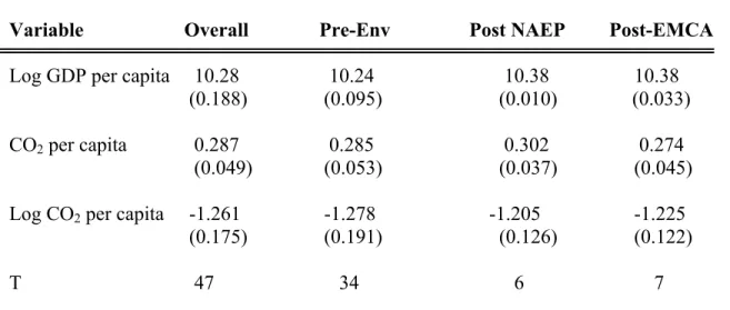
Table 1 below gives the descriptive statistics of the variables that are used in this analysis. This is done for the overall sample and also for three environmental dispensations. Pre-Env period refers
3 An acf with large spikes at initial lags that decays to zero or a pacf with a large spike at the first and
possibly at the second lag indicates an autoregressive process. An acf with a large spike at the first and possibly at the second lag and a pacf with large spikes at initial lags that decay to zero indicate a moving average process. If both the acf and pacf exhibiting large spikes that gradually die out, this indicates both autoregressive and moving averages processes
to the years before 1994 when the first environmental initiative came into place namely National Environmental Policy (NAEP). Post-NAEP is the period after 1994 but before 1999 when Environmental Management Act was enacted. Post-EMCA is the period after Environmental Management Act was enacted which established National Environmental Management Authority (NEMA) and is more rigorous with environmental management.
Table 1: Summary statistics for EKC Hypothesis
Variable Overall Pre-Env Post NAEP Post-EMCA
Log GDP per capita 10.28 10.24 10.38 10.38 (0.188) (0.095) (0.010) (0.033) CO2 per capita 0.287 0.285 0.302 0.274
(0.049) (0.053) (0.037) (0.045) Log CO2 per capita -1.261 -1.278 -1.205 -1.225
(0.175) (0.191) (0.126) (0.122) T 47 34 6 7 Source: Authors computation from World Development Indicators 2006 Database
The figures in parentheses are the standard deviation
4.2: Trend Analysis of Economic Growth and Environmental Quality for Kenya
This section presents the trends of indicators of economic growth and environmental quality. Understanding these trends is important for exploring Environmental Kuznets Curve hypothesis which postulates that at lower levels of income, emissions which are the indicators of environmental quality tend to increase with an increase in income while at higher levels of income, emissions tend to fall with income. It would be important therefore from the onset to examine the trends of each if this variables before embarking on any analysis.
GDP is a measure of national income. It measures the value of output within a country and is considered as the broadest indicator of economic growth. However, GDP per capita is considered to be a more reliable indicator of economic growth because takes the size of population into consideration. The manufacturing sector is a major contributor of GDP. In Kenya it accounts for 13% of GDP annually. While the trend of GDP has been steadily increasing in Kenya, the contribution of the manufacturing sector to GDP has been fluctuating over the same period with very little upward growth. This is shown in figure 2 below.
Figure 2: Trend of GDP and Manufacturing Value Added in Kenya
0.00 200000.00 400000.00 600000.00 800000.00 1000000.00 1200000.00 1971 1973 197 5 197 7 1979 1981 198 3 1985 198 7 1989 1991 199 3 1995 1997 1999 200 1 YEARS G D P /M V A IN M IL L IO N S
GDP in millions Manufacturing, VA in millions
Linear (GDP in millions ) Linear (Manufacturing, VA in millions)
Analyzing the trend of GDP per capita and MVA per capita, between 1970 and 1982, they had a uniform trend with GDP per capita growing faster than MVA per capita. However, for the rest of the period, they tend to moved in opposite directions. This is shown in figure 3 below.
Figure 3: Trend of GDP per capita and MVA per capita 20 00 25 00 30 00 35 00 40 00 M V A /C ap it a (i n m ill io n s K sh s) 2 600 0 280 00 30 00 0 32 000 3 400 0 G D P pe r c a pi ta ( in m ill io n s K sh s .) 1970 1980 1990 2000 Year
GDP per capita MVA/Capita
Another important aspect of growth is the actual growth rate of both the GDP and MVA. Looking at both the growth rate of GDP and the growth rate of manufacturing value added in figure 4 below, it is clear that despite the upward trend, there have been periods of accelerated growth and slanting growth. Between 1971 and 1977, growth rates of both GDP and MVA were on the downward trend. There was a temporary upward trend in 1977 before another decline in 1979 to 1983. In the periods 1984/1985 and 1993/1994, MVA grew faster than GDP. Indeed 1993/1994 experienced negative GDP growth. Between 1999 and 2001, there was a negative growth in MVA.
Figure 4: Growth rates of GDP and MVA
-5 0 5 10 15 20 25 30 35 1971 1974 1977 1980 1983 1986 1989 1992 1995 199 8 2001 YEARS GR OW T H R A T E S GDP Manufacturing, VA
Analyzing the trend of emissions in figure 5 below, it is clear that the emissions do not exhibit a uniform trend.
Figure 5: Trend of CO2 emissions per capita
0.00 0.05 0.10 0.15 0.20 0.25 0.30 0.35 0.40 0.45 1971 1973 1975 1977 1979 1981 1983 1985 1987 1989 1991 1993 1995 1997 1999 2001 YEARS CO 2 E M M IS SI O NS P E R CAP IT A
From the figure, it is observed that before 1980, the trend is fluctuating but on an upward trend. Between 1980 and 1985, they were on a downward trend a period that coincides with a downward trend in the growth of MVA. This is not surprising because the growth in the manufacturing sector is associated with increased air pollution. Between the year 1986 and 1994, the levels of CO2 emissions were constant a period that also saw uniform growth in MVA.
Another upward trend is observed in 1995/1997 coinciding with both an increase in MVA growth as well as that of GDP. In 1998/1999, a sharp fall in both CO2 emissions and water
pollutants. Interestingly, it was this same period that MVA growth rate dropped sharply but this was accompanied with a sharp rise in GDP growth rate. This was followed by a jump in both CO2 emissions and water pollutants in 1999/2000 followed by a period of constant both CO2
From the analysis above, there seems to be a close connection between the growth in MVA and CO2 emissions. This is expected because the manufacturing sector is known to be one of the
sources of air pollutants. The reason why the sector is associated with pollution is because of overdependence of fossil fuel. It is therefore of interest in this study to explore the relationship between CO2 emissions and energy use. This is summarized in figure 6 below
Figure 6: Relationship between per capita CO2 emissions and energy use
.5 .5 5 .6 .6 5 E ner gy us e/ c a pi ta ( k t o f o il equ iv al ent ) .2 .2 5 .3 .3 5 .4 C O 2 e m is s ions /c api ta ( m e tr ic t on s ) 1970 1980 1990 2000 Year
CO2 emissions/capita Energy use/capita
It is revealed that energy use per capita is declining while the CO2 per capita is fluctuating. For the period between 1970 and 1980, the emissions per capita were quite high averaging at 0.299. In the 1980s they fell to an average of 0.247 before rising again in the 1990 to an average of 0.273. In the year 2001, there is already a downward trend. The CO2 emissions seem to move in
cyclical movements which cannot be associated with the level of energy use from the graph. The Environmental Kuznets Curve hypothesis which is the subject matter in this analysis postulates that at low levels of income, emissions are rising with income but as income rises above a certain level, emissions will be decreasing with rise in income. To assess this, CO2 per
Figure 7: Trend of CO2 emissions per capita and GDP per capita .2 .2 5 .3 .3 5 .4 C O 2 /c api ta ( in m et ri c t ons ) 26000 2 8000 30 000 32000 3 4000 G D P per c api ta ( in m illio n K s h s .) 1970 1980 1990 2000 Year
GDP per capita CO2 emissions per Capita
There is no systematic trend for any of the two variables which provides no support for the Environmental Kuznets Curve hypothesis. Plotting Emissions per capita against GDP per capita in figure 8 provides no support for the hypothesis.
Figure 8: Relationship between CO2 per capita and GDP
0.00 0.05 0.10 0.15 0.20 0.25 0.30 0.35 0.40 0.45 26548 3062 0 29869 31016 3311 6 33633 32048 3156 1 3333 4 34584 3423 3 3204 4 32459 3228 5 3255 4 32710 GDP PER CAPITA CO 2 E M IS SI O NS P E R C AP IT A
The graphical analysis is not sufficient to conclude the behaviour of Environmental Kuznets Curve, An econometric analysis of this relationship is more reliable which is presented in the next section.
4.3: Econometric Analysis
4.3.1: Stationarity Analysis
In this section we focus on the time series properties of the natural log of GDP/Capita, natural log of squared GDP/Capita and natural log of CO2/Capita and test whether the series are
stationary or not. Most macroeconomic variables tend to be non-stationary and are also likely to be trended or integrated. This means that the variables may have a mean that changes with time and a non-constant variance. Regression involving such non-stationary series can falsely imply the existence of a meaningful relationship. Before embarking on any analysis, it is therefore important to test if the variables are stationary and if not at what level they become stationary. The test for stationarity involves establishing whether a time series follow a unit-root process. The presence of a unit root implies that the series is non-stationary.
The Unit root process is implemented using two different tests. The first is the Augmented Dickey-Fuller test (ADF) whose null hypothesis is that the variable contains a unit root thus non-stationary, and the alternative is that the variable was generated by a stationary process. Using both the Akaike Information Criterion (AIC) and the Schwarz’s Bayesian Information Criterion (BIC), a decision is made as to what is the optimal number of lags since the lag length is known to affect the power properties of the ADF test. The second test is the Phillips-Perron test.
All the two tests are implemented with trend and without trend and the results are reported in table 2 below.
Table 2: Unit Root Tests for variables in levels
Variable GDP/Capita (GDP/Capita)2 CO2/Per Capita
Trend No Trend Trend No Trend Trend No Trend
ADF (Lags = 0) -1.380 -1.795 -1.639 -0.202 -2.347 -2.418 (Optimal lags) -2.613* -2.712* -0.413 -0.621 -2.545 -1.906 (1st Difference) -7.346***-6.810*** -7.150*** -6.862*** -7.389*** -7.450*** Phillip-Perron (Lags = 0) -1.336 -1.812 -1.616 -0.229 -2.458 -2.523 (1st Difference) -7.428*** -6.782*** -7.171***-6.836*** -7.402*** -7.461***
Source: Authors computation from World Development Indicators Database
Variables in logs. *, indicates significance at 10% level, **, at 5% level and ***, at 1% level
The results in table 2 show that the natural log of CO2/capita and the natural log of squared
GDP/capita are non-stationary both at levels and when optimal lag length is considered. They are also trend non-stationary. In the case of the natural log of GDP/capita, it is marginally stationary at optimal lag length but non-stationary at levels. However, all the variables are both trend and level stationary in first difference. The results from Phillip Perron test confirm that all the three variables are integrated of order 1.
It is well known in econometric literature that the presence of structural breaks in a time series may render the results of a unit root rest to be invalid, rejecting the null hypothesis even when the series are non-stationary. It is therefore important to check the results of unit root analysis presented above by a third method, Zivot and Andrews test (Zandrews test), which tests for unit root while taking into account the possibility of structural breaks in the data. From the results of the Zandrews test, a single structural break for each of the series is identified. For the natural log of GDP/capita, the break is in 1971 and the t-statistic of -4.779 is less than the critical value at
5% level reading to the acceptance of the null hypothesis of non-stationarity; hence the variable is non-stationary. For the natural log of squared GDP/capita, the break is in 1971 and the t-statistic of -4.560 is less than the critical value at 5% level reading to the acceptance of the null hypothesis of non-stationarity. For the natural log of CO2/capita, the break is in 1992 and the t-statistic of -2.710 which is less than the critical value at 5% leads to the acceptance of the null hypothesis. Hence, even when structural break is considered, all the three variables are non-stationary.
4.3.2: Cointegration analysis
This section seeks to establish the dynamic relationship between GDP/Capita and CO2/Capita. This involves establishing if the two non-stationary processes have the same stochastic trend which is done by testing if the two variables are cointegrated. This is because even though individual time series are non-stationary, their linear combination could be stationary because equilibrium forces tend to keep them together in the long run. If this be the case, the variables are said to be cointegrated and an error correction term exist to distinguish short-term deviations from the long-term equilibrium relationship implied by the cointegration.
There are two tests to test for cointegration; Engle_Granger Methodology for single equation models due to Engle and Granger (1987) and the Johansen procedures for multiple equation systems developed by Johansen (1995). To implement the Engle-Granger approach, the cointegrating equation is first estimated by regressing the first difference of CO2/capita on
GDP/capita and first difference of squared GDP/capita (all variables in natural logs) after which the residuals from the regression are checked if they are integrated by applying the ADF test for
unit root. The results (ADF = -7.461***) reveal that the residuals have no unit root and hence are stationary which implies that the variables are cointegrated.
The next step is to identify the number of cointegrating equations using the Johansen approach. The results reveal that the Johansen’s trace statistic at r = 0 of 73.44 is greater than its critical value of 29.68 rejects the null that the variables are not cointegrated. Further, the null hypotheses that r = 1 and r = 2 are also rejected with trace statistics being greater than the critical values. Hence the null hypothesis of cointegrating equations being greater than 2 cannot be rejected.
4.3.3: The Error Correction Model
The cointegration analysis describes the long-run relationship between CO2/Capita, GDP/Capita
and squared GDP/Capita. Next is to estimate an error correction model (ECM). The ECM approach allows us to explain changes in the CO2 emissions in terms of changes in GDP, as well
as deviations from the long-run relationship between the two variables.
Following Engle and Granger (1987), if the two time series are cointegrated, then they can be represented by an error correction representation of the form
0 1 1 ( )E t β β ( )Y t ηut− t Δ = + Δ + +ε ( ) ( ) t t Y ………..(5.7)
where u denotes the equilibrium error term defined as, u−1 = E −1−α α0− 1 t−1, εt indicates the error term and η < 0 is the error correction parameter, representing the principle of negative feedback. β1 is the parameter capturing any immediate effect that GDP may have on CO2 emissions while the term η captures the speed at which the dependent variable responds to any discrepancy from the long-run equilibrium condition. Therefore, the error correction parameter η
ties the short-run changes in CO2 emissions to the long-run effects through a feedback mechanism.
Estimating the error correction model, it is revealed that η, the coefficient of error correction term has the expected sign and is significant at 5% level of significance. The magnitude of η is 1.09 which means that the speed of adjustment for CO2 to its long-run equilibrium is 109%.
4.3.4: Granger Causality Tests
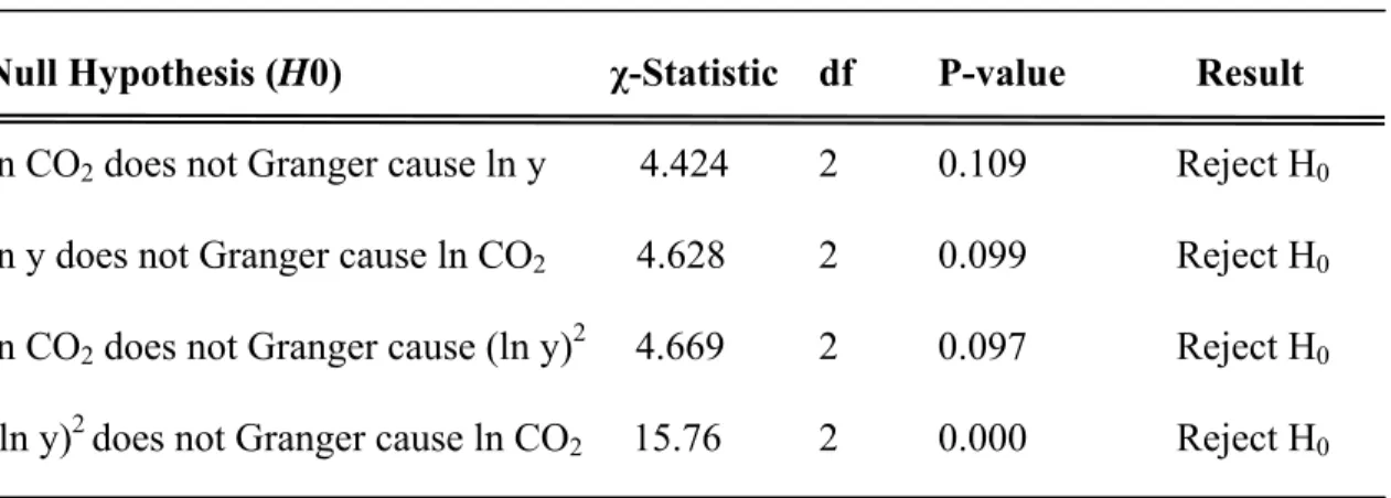
Having established a long-run relationship between carbon emissions and GDP, it is important to determine if there exists a causal relation between the variables. In order to identify the direction of the relationships, the causality test for the three variables is conducted using the pair wise Granger causality test the results of which are reported in table 3 below.
Table 3: Pair Wise Granger Causality Wald Tests
Null Hypothesis (H0) χ-Statistic df P-value Result
ln CO2 does not Granger cause ln y 4.424 2 0.109 Reject H0
ln y does not Granger cause ln CO2 4.628 2 0.099 Reject H0
ln CO2 does not Granger cause (ln y)2 4.669 2 0.097 Reject H0
(ln y)2 does not Granger cause ln CO2 15.76 2 0.000 Reject H0
Source: Estimated using Stata 10
The critical value at 95% confidence level with 2 degrees of freedom is 5.991 which is less than the computed values. This implies that the null hypothesis that there is no causality between the variables is rejected for all the four relationships. This is also confirmed by the P-values which
are all less than 0.05. From these results, a two dimensional causal relationship exists between carbon emissions and GDP and its squared transformation.
4.3.5: Testing the EKC Hypothesis for CO2 Emissions
As mentioned earlier, simple OLS regression with non-stationary series is likely to lead to spurious results not unless the two series are cointegrated. In the presence of cointegration, OLS is a valid estimation procedure resulting in super-consistent estimators (see Friedl and Getzner, 2003). Therefore, for this analysis, since the series are cointegrated, OLS is a valid method to estimate the Environmental Kuznets Curve equation
To test for the evidence of the Environmental Kuznets Curve hypothesis in Kenya, a quadratic relationship between carbon dioxide emissions and GDP is estimated. The quadratic model is expressed in the form
2
0 1 2 3
t t t
E =β +βY +β Y +β X +εt ………..(5.8)
where is the natural logarithm of carbon emissions per capita, is the natural logarithm of GDP per capita,
t
E Yt
t
X is a structural break dummy variable. εt is the error term whileβi are parameters to be estimated. As discussed earlier, an inverted-U relationship between GDP and CO2 requires that β1 >0 andβ2 <0. Furthermore, the two parameters must be statistically
significant. The estimation progresses in steps by first estimating a linear relationship followed by a quadratic relationship. The variables are estimated in first difference. The results are shown in table 4 below.
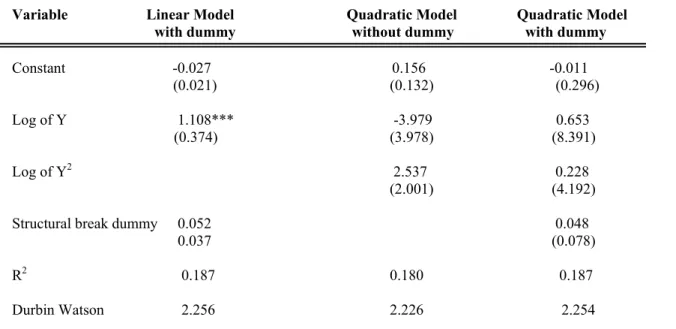
Table 4: EKC Model Estimation Results
Variable Linear Model Quadratic Model Quadratic Model
with dummy without dummy with dummy Constant -0.027 0.156 -0.011 (0.021) (0.132) (0.296) Log of Y 1.108*** -3.979 0.653 (0.374) (3.978) (8.391) Log of Y2 2.537 0.228 (2.001) (4.192) Structural break dummy 0.052 0.048 0.037 (0.078)
R2 0.187 0.180 0.187
Durbin Watson 2.256 2.226 2.254 N = 46
Source: From Pooled OLS estimation using Stata 10. The figures in parentheses are the standard errors. ***,**, and * denote Significance levels at 1% , 5% and 10% respectively based on t-statistics.
Estimating a linear model without considering structural breaks shows a significant positive coefficient of GDP per capita and an R2 of 0.149. Including the dummy variable for structural break in the estimation, the results show a significant positive coefficient of GDP per capita and an R2 of 0.187. The constant is negative and insignificant. A low R2 casts doubts on the fitness of
the model. To try to improve this, a quadratic form of the model is estimated. Without considering the structural breaks, the coefficient of GDP per capita is negative and with very large standard error which lenders it insignificant. The coefficient of squared GDP per capita is positive and with very large standard error which lenders it insignificant. The constant term is positive but insignificant while the R2 is 0.179. Considering the quadratic model with structural
breaks, the coefficient of GDP per capita is now positive but insignificant due to large standard errors. The coefficient of squared GDP per capita remains positive and insignificant while the constant term is now negative. The R2 is 0.187, hence the model has very low explanatory
powers implying that the income level, though significant, is not a major determinant of the level of carbon emissions in this analysis. The fact that the coefficient of GDP per capita in the linear model is significant and positive is suggestive that as GDP grows, the level of carbon dioxide emissions increases.
In order to determine if the Environmental Kuznets Curve hypothesis holds, an examination of the magnitudes and signs of the coefficients of GDP per capita and its square follows for the linear and quadratic model with dummy variables, reported in table 4. Examining the coefficients of GDP per capita in the linear model, β1 is positive and significant. For the quadratic model, both β1 and β2 are positive and insignificant. The fact that only the β1 of the linear model is significant allows the interpretation of the linear model only. Having β1>0 as significant and
2 0
β > as insignificant is indicative of a monotonically increasing relationship between income and carbon dioxide emissions. This relationship can be shown graphically as in the figure 9 below.
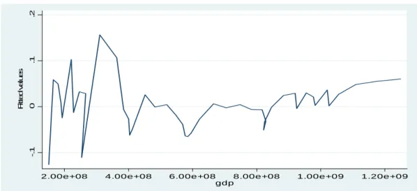
Figure 9: Regression Line for the Relationship between fitted CO2 Emissions and GDP
-. 1 0 .1 .2 Fi tt e d v a lu e s
2.00e+08 4.00e+08 6.00e+08 8.00e+08 1.00e+09 1.20e+09 gdp
The figure shows a cyclical relationship which begins as an inverted-U relationship before giving way to a U-shaped4 relationship. This is suggestive of an N-shaped relationship with multiple cycles. Given this interesting relationship, it would be good to predict the future path of carbon emission which is the task of the next section.
4.4: Forecasting the Future Path of Carbon Emissions in Kenya
In this section, we apply the Box-Jenkin’s ARIMA methodology to carbon dioxide emissions for Kenya. Figure 10a below plots the original data for carbon dioxide emissions. From the figure, the time series of carbon dioxide emissions is non-stationary. To make the series stationary, the differencing process follows which identifies the series to be stationary at first difference (see figure 10b below).
Figure 10: Time Series of Ln CO2 per Capita
a) in levels b) in first difference
.2 .2 5 .3 .3 5 .4 CO 2_ c a 1960 1970 1980 1990 2000 2010 Year -. 1 -. 0 5 0 .0 5 C O 2_c a, D 1960 1970 1980 1990 2000 2010 Year
The results of the correlogram, which shows autocorrelations between per capita carbon dioxide emissions and its lagged values, at levels and in first difference reveals that the series is an AR(1) process. The variable is log transformed to eliminate variance non-stationarity.
The next step is to estimate the best ARIMA model for carbon dioxide emissions in first difference. The parameters are estimated using function minimization procedures so that the sum of squared residuals is minimized. The identification of the model is done using AIC and BIC criteria where out of three specifications, ARIMA (1 1 0) is identified as the best because it reports the lowest AIC and BIC values. The estimates of the parameters are used in the forecasting stage to calculate new values of carbon dioxide emissions. The results of the forecasted model are reported in table A5.1 in appendix 5.1. It is observed that the forecasting values generated by the proposed model follows the pattern of the original series which attests to the accuracy of the model. This is clear from the figure 11 below
Figure 11:Static and Dynamic Forecasts: Actual and Forecasted Value of CO2 Emissions
-2 -1 0 1 2 3 1960 1980 2000 2020 2040 2060 Year
lnCO2_ca y prediction, dyn(2006)
The trends fit very well and they move together hence, the overall quality of the model is good. However, although the model generates reasonable one–step–ahead forecasts, the dynamic form of the model is quite unsatisfactory in the sense that a large portion of the forecast horizon gives very low predicted values.
Another way to check for the reliability of the model is by plotting the corelogram of the residuals and examining for serial correlation. Testing the residues for serial correlation reveals that they are statistically independent. Plotting the residues in figure 12 also shows that they are small and oscillating around zero
Figure 12: One Step residuals for forecasted Model
-. 4 -. 2 0 .2 .4 re si du al , on e -s te p 1960 1980 2000 2020 2040 2060 Year
Another important factor is the confidence limit for the forecasted model. The upper confidence limit is reported as +0.340 and the lower limit as -0.338. As mentioned earlier, any forecasted values within the confidence limit are satisfactory.
5.0: Conclusion and Recommendations
This study sought to explore the validity of Environmental Kuznets Curve hypothesis for Kenya in the case of carbon emissions. There is no evidence that the hypothesis holds but rather an increasing but cyclical behaviour is observed. Predicting the future trend of carbon emissions, a monotonically increasing trend is observed for carbon emissions. The results suggest that Environmental Kuznets Curve hypothesis is not relevant for policy formulation in Kenya given its low level of development. However, there is some evidence that if the government has the right environmental legislation and institutional framework, then Environmental Kuznets Curve hypothesis could be a reality. This raises another interesting question; whether the cyclical behaviour of the environmental Kuznets curve was due to the absence of or poor monitoring of environmental quality such that the information on emissions was inaccurate. This is a likely scenario because the countries that have reported evidence of the hypothesis have existed for many years and there is no indication at what level of development they realized the upward trend or if there were any preconditions for this relationship. However, this remains an empirical question.
It is therefore important for Kenya, and most African countries, to be cautious in embracing the Environmental Kuznets Curve hypothesis as a policy tool because the economy is still young and the legal and institutional framework for environmental management are in their formative stages. Given these shortcomings, it may not be possible to realize any positive environmental benefits from exploiting the environment in the name of economic growth. It is therefore recommended that in order to ensure sustainable development, environmental policies must be pursued vigorously alongside economic development policies.
6.0: References
Arrow, K., Boling, B., Costanza, R., Dasgupta, P., Folke, C., Holling, S., Jansson, B.O,
Levin, S., Mäler, K.-G., Perrings, C., Pimentel, D., 1995, “Economic Growth, Carrying Capacity and the Environment”, Science 268, 520-521.
Bennett, J.W, Gillespie, R and Dumsday, R, 2008, ‘Australian economic development and the environment: conflict or synergy?’, 52nd Conference, Canberra, Australia, No 6040
Bertinelli, L., and E. Strobl , 2005, “The Environmental Kuznets Curve Semi-Parametrically Revisited,” Economics Letters, 88, 350-357.
Carson, R. T., Y. Jeon and D. McCubbin, 1997, “The Relationship Between Air Pollution Emission and Income,” US Data. Environmental and Development Economics 2:433-450.
Chertow, M.R., 2001, “The IPAT Equation and Its Variants Changing Views of Technology and Environmental Impact”, Journal of Industrial Ecology, 4 (4):13-29.
Cole, M. A., A. J. Rayner and J. M. Bates, 1997, “The Environmental Kuznets Curve: An Empirical Analysis, Environmental and Development Economics 2:401-416.
Commoner, B., 1972, The environmental cost of economic growth. In Population, Resources and the Environment, edited by R. G. Ridker. Washington DC: U.S. Government Printing Office, pp. 339–363.
Dasgupta, S, Laplante, B., Wang, H. and Wheeler, D., 2002, “Confronting the Environmental Kuznets Curve”, Journal of EconomicPerspectives, 16 (1), 147 - 168.
De Bruyn, S.M., van den Bergh, J.C.J.M., Opschoor, J.B., 1998, “Economic Growth and Emissions: Reconsidering the Empirical Basis of Environmental Kuznets Curves”, Ecological Economics 25, 161-175.
De Bruyn, S.M., Heintz, R.J., 1999, “The Environmental Kuznets Curve Hypothesis”, in van den Bergh, J.C.J.M., (Ed.), Handbook of Environmental and Resource Economics, Edward Edgar, Cheltenham, UK, 656-677.
Dijkgraaf, E., & Vollebergh, H. R. J.,1998, “Growth and/or Environment - Is There a Kuznets Curve for Carbon Emissions?”, 2nd ESEE Conference, Université de Génève.
Egli, H., 2004, “The Environmental Kuznets Curve: Evidence From Time Series Data for Germany”, Working Paper 03/28, Institute of Economic Research.
Ehrlich, P. and J. Holdren, 1971, “Impact of Population Growth”, Science 171: 1212–1217
Encyclopedia.com, 2008, Environmental Kuznets Curves." International Encyclopedia of the Social Sciences.
Engle, R.F., Granger, C.W.J., 1987, “Cointegration and Error Correction: Representation, Estimation and Testing”, Econometrica 55, 251-276.
Friedl, B., Getzner, M., 2003, “Determinants of CO2 Emissions in a Small Open Economy”,
Ecological Economics 45, 133-148.
Grossman, G.M., Krueger, A.B., 1991, “Environmental Impacts of a North American Free Trade Agreement”, NBER Working Paper No. 3914.
Grossman, G.M., Krueger, A.B., 1995, “Economic Growth and the Environment”, The Quarterly Journal of Economics 110, 353-377.
Harbaugh, W.T., A. Levinson and D.M. Wilson, 2002, “Reexamining the Empirical Evidence for an Environmental Kuznets Curve”, The Review of Economics and Statistics, 84(3), 541-551. Hettige, H., Mani, M. and Wheeler, D., 1997, “Industrial Pollution in Economic Development: Kuznets Revisited” Development Research Group World Bank.
Johansen, S., 1995, “Likelihood-Based Inference in Cointegrated Vector Autoregressive Models, Oxford University Press, Oxford.
Kuznets, S., 1955, “Economic Growth and Income Inequality”. American EconomicReview 45, 1-28.
Levinson, A., 2000, "The Ups and Downs of the Environmental Kuznets Curve"
Lindmark, M.,2002,, An EKC-Pattern in Historical Perspective: Carbon Dioxide Emissions, Technology, Fuel Prices and Growth in Sweden, 1870-1997”, Ecological Economics,42: 333-347.
MAPC, 2010, Smart Growth Principles, Metropolitan Area Planning Council, Promoting Smart Growth and Regional Collaboration. Metropitan Area Planning Council
Moomaw, W.R. and Unruh, G.C.,1997, “Are environmental Kuznets Curves Misleading Us? The Case of CO2 Emissions”, Environment and Development Economics, 2, 451-463.
Olusegun, O.A., 2009, Economic Growth and Environmental Quality in Nigeria: Does Environmental Kuznets Curve Hypothesis Hold?, Environment Research Journal, 3 (1), 14-18 Panayotou, T., 1993, “Empirical Tests and Policy Analysis of Environmental Degradation at Different Stages of Economic Development”, Working Paper WP238 Technology and Employment Programme, Geneva: International Labor Office.
Panayotou, T.,1997,. “Demystifying the Environmental Kuznets Curve: Turning A Black Box into a Policy Tool”, Environmental and Development Economics 2:465-484.
Pasche M., 2002, “Technical Progress, Structural Change, and the Environmental Kuznets Curve, Ecological Economics. N 42. pp. 381-389.
Rostow, W.W., "The Five Stages of Growth--A Summary," in The Stages of Economic Growth: A Non-Communist Manifesto, Cambridge: Cambridge University Press, 1960, Chapter 2, pp. 4-16
Selden, T.M., Song, D., 1994, “Environmental Quality and Development: Is there a Kuznets Curve for Air Pollution Emissions?”, Journal of Environmental Economics and Management 27, 147-162.
Shafik, N., 1994, “Economic Development and Environmental Quality: An Econometric Analysis” Oxford Economic Papers 46: 757-773.
Shafik, N., Bandyopadhyay, S., 1992, “Economic Growth and Environmental Quality: Time Series and Cross-Country Evidence” Background Paper for World Development Report, World Bank, Washington, DC.
Stern, D.J., Common, M.S., Barbier, E.B., 1996, “Economic Growth, Trade and the
Environment: Implications for the Environmental Kuznets Curve. World Development 24, 1151-1160.
Vincent, J. R., 1997, “Testing For Environmental Kuznets Curves Within a Developing Country”, Environmental and Development Economics 2:417-431.
World Bank, 2006, "World Development Indicators 2006 World Bank, 2009, "World Development Indicators 2009