Abstract— This contribution develops a new numerical method to analyze fluid-structure interaction (FSI), based on smoothed particle hydrodynamics (SPH). In this way, fluid and elastic structure continua are coupled using a monolithic but explicit numerical scheme. The proposed method is similar to so-called SPH projection method and consists of two steps. The first step plays the role of prediction, whereas in the second step incompressibility constraint is satisfied. Problem of imposing no-slip boundary condition on deformable walls is investigated. The proposed method is employed to simulate a pulsatory flow moving through flexible walls which mimics unsteady blood flow in arteries.
Index Terms— Smoothed particle hydrodynamics (SPH), Fluid-structure interaction (FSI), Meshfree method, Lagrangian method, no-slip boundary condition
I. INTRODUCTION
Numerical analysis can significantly reduce time and cost by replacing many expensive and elaborate experiments with virtual simulations. In the bioengineering area, dealing with the living organism in vivo not only is associated with many technical difficulties, but also provokes ethical and moral problems. From the other point of view, large parts of human body consist of fluids, which are interacting with flexible organism. Study of body fluids in human is called Hemodynamics. However, in the numerical fields these problems, in which fluid and structures interact with each other, are called fluid-structure interaction (FSI).
All other past-proposed methods for the numerical simulation of FSI are based on discretization of computational domain using mesh. Mesh generation is a delicate technique, which is highly important when dealing with complex geometries. Generally, there are two classes of mesh-based methods namely fixed-grid methods and deforming-grid methods [1]. Deforming-grid methods usually need remeshing, particularly when large deformation is of great interest, however remeshing strategy can be a difficult and time consuming task [1,2]. On the other hand, fixed-grid methods usually require an interpolation to the immersed boundary, which result in inaccurate computations in vicinity of these boundaries [2].
Smoothed particle hydrodynamics (SPH) is a meshfree and
Manuscript received March 3, 2008.
M. H. Farahani recently received his MSc. from Department of Mechanical Engineering, Faculty of Engineering, University of Guilan, Rasht, 3756 IRAN (e-mail: [email protected]).
N. Amanifard, is with Department of Mechanical Engineering, Faculty of Engineering, University of Guilan, Rasht, 3756 IRAN. (Corresponding author; phone: 98-131-6690274-8; fax: 98-131-6690271; e-mail:
Gh. Pouryoussefi is with Department of Aerospace Engineering, K.N. Toosi University of technology, Tehran 16765-3381 IRAN, ([email protected]).
Lagrangian method by which problems associated with mesh can be treated. Ability of SPH to simulate each of fluid dynamic problems as well as elastic plastic deformation of solids has been demonstrated. Recently some researches have been devoted to utilize SPH to simulate FSI problems [3,4]. Hence, by using SPH, we can couple fluid and structure using a monolithic approach. Antoci et al. [3] were the first who used standard SPH to simulate FSI problems. On the other hand, Hosseini et al. [4] developed a three-step SPH-projection method, which had already been proposed by Hosseini et al. [5], to simulate FSI problems. Their proposed method included a new SPH algorithm for simulation of elastic deformations of solids. A comparison with experiments illustrates that the results which were reported by Hosseini et al. [4], in deformation simulation of an elastic gate subjected to water pressure, were more accurate than the results which were reported by Antoci et al. [3].
Indeed, neither Hosseini et al. [4] nor Antoci et al. [3] considered the no-slip boundary conditions in their simulations. In the current work, the problem of imposing the no-slip boundary condition on moving walls is studied. In this way, the three-step algorithm of Hosseini et al. [4,5] is modified according to the viscosity term which was proposed by Moriss et al. [6]. The modified algorithm is used to simulate an internal pulsatory flow moving through flexible walls, which mimics blood flows in arteries.
II. GOVERNING EQUATIONS
A. Fluid domain
The fluid is assumed to be isothermal and incompressible and the governing equations within the fluid domain in absence of body forces, are given by
j j
x
u
Dt
D
∂
∂
−
=
ρ
ρ
(1)
j j
ij i
x
P
x
Dt
Du
∂
∂
−
∂
∂
=
ρ
τ
ρ
1
1
(2)
where
ρ
,t
,u
j, p, andτ
ij denotes the density, time, velocity, pressure, and shear stress tensor respectively. Moreover,x
jis thej
th component of position vector. B. Solid domainThe momentum equation for an elastic body in absence of body forces is
j ij i
x
Dt
Du
∂
∂
=
σ
ρ
1
, (3)
where
σ
ij is the stress tensor which can be written asNumerical Simulation of a Pulsatory Flow
Moving Through Flexible Walls Using
Smoothed Particle Hydrodynamics
ij ij ij
S
P
+
−
=
δ
σ
, (4)where
S
ij is the deviatoric stress tensor. The deviatoric stress can be presented by assuming linear elastic theory and considering Hook’s law as [7]kj ik jk ik ij ij ij ij
S
S
G
t
D
S
D
ω
ω
ε
δ
ε
−
+
+
=
3
1
2
, (5)where
G
is the shear modulus. The strain rate tensorε
ij, and rotation tensorω
ij are defined as∂
∂
+
∂
∂
=
i j j i ijx
u
x
u
2
1
ε
, (6)∂
∂
−
∂
∂
=
i j j i ijx
u
x
u
2
1
ω
. (7)Substituting (4) into (3) yields
j j ij i
x
P
x
S
Dt
Du
∂
∂
−
∂
∂
=
ρ
ρ
1
1
. (8)
III. METHODOLOGY
The foundation of SPH is based on interpolation theory. According to the aforementioned theory, any field variable
A
can be defined over a domain of interest in terms of its values at a set of discrete disordered points (so-called SPH particles) by suitable definition of an interpolation kernel. These particles carry the material properties such as density, velocity, pressure, stress etc. The exact integral representation ofA
is( )
r
( ) (
r
r
−
r
′
)
r
′
Ω
′
=
A
δ
d
A
, (9)where
δ
(
r
−
r
′
)
is the Dirac delta function andΩ
is the computational domain. Equation (9) can be represented by integral interpolation of the quantity A as( )
r
( )
r
(
r
−
r
′
)
r
′
Ω
′
≈
A
W
,
h
d
A
, (10)where
h
is smoothing length proper to kernel function W which represents the effective width of the kernel. The kernel has the following properties [8](
)
(
−
′
)
=
(
−
′
)
=
′
′
−
→
r
r
r
r
r
r
r
δ
h
W
d
h
W
h V,
lim
1
,
0. (11)
There are many possible choices of kernel function. A quintic kernel is used in the following simulation [6]
( )
≥
<
≤
−
<
≤
−
−
−
<
≤
−
+
−
−
−
=
,
3
,
0
;
3
2
,
)
3
(
;
2
1
,
)
2
(
6
)
3
(
;
1
0
,
)
1
(
15
)
2
(
6
)
3
(
478
7
,
5 5 5 5 5 5s
s
s
s
s
s
s
s
s
s
h
r
W
π
(12) whereh
s
=
r
. The dominant error term in the integralinterpolant is
O
( )
h
2 .If
A
( )
r
′
is known only at a discrete set ofN
pointN
r
r
r
1,
2,...,
then the interpolation of quantityA
can be approximated by a summation interpolant as follows [8]( )
Nm
bW
(
h
)
b b b
h
A
,
A
1
r
r
r
≈
=−
′
ρ
, (13)where the summation index b denotes a particle label and particle b carries a mass
m
bat the positionr
b. The value ofA
atb
−
th
particle is shown byA
b.Derivative of A with respect to
x
is given by [9](
)
∂
∂
−
Φ
Φ
=
∂
∂
b ab a b b b b a ax
W
m
x
A
A
A
ρ
1
, (14)
where
Φ
is any differentiable function.IV. SOLUTION ALGORITHM
In this section, the fully explicit three-step algorithm of Hosseini et al. [4] will be modified to consider no-slip boundary condition on moving walls. The first two steps of the aforementioned algorithm play the rule of prediction part of pressure projection methods (e.g. see [10]) and the third one is a correction. Since in the first step only body forces should be taken into account, in absence of body forces, it can be neglected. Hence, the algorithm is reduced to two following consecutive steps.
A. First step (Prediction)
Solid: In this step for solids, divergence of deviatoric stress tensor is calculated. In this way first, the deviatoric stress tensor is calculated according to constitutive equation (5), then the divergence of deviatoric stress tensor
T
i is given by(
h
)
W
S
S
m
x
S
T
a abb ij b a ij a b b a j ij i
,
1
22
+
⋅
∇
r
=
∂
∂
=
ρ
ρ
ρ
,(15)where
r
ab=
r
a−
r
band(
)
(
j)
b i a ab ab ab
a
x
x
d
dW
h
W
=
−
∇
r
r
r
,
1
. (16)Fluid: In this step for fluids, divergence of shear stress tensor should be calculated. Hosseini et al. [4], [5] calculated the shear stress tensor using the second principal invariant of the shear strain rate tensor, nevertheless, it can be simply investigated that the resulted velocity profile for the Poiseuille problem is inaccurate near the boundaries. Morris et al. [6] suggested another form of the viscous term
(
)
a abi ab ab b a i ab b a b b a j ij i
w
x
u
m
x
S
T
⋅
∇
+
+
=
∂
∂
=
1
(
2)
2η
ρ
ρ
µ
µ
ρ
r
.(17)Although the above form does not satisfy angular momentum [11], provides accurate results near the boundaries.
to a new temporary position.
t
T
u
u
~
i=
ti−∆t+
i∆
, (18)t
u
x
x
ti t i i∆
+
=
−∆~
~
. (19)
B. Second step (Correction)
There was no constraint to impose incompressibility effect in the previous step, thus particle movements have changed density of the particles. Density variations can be calculated using the continuity equation. Choosing
Φ
=
1
,A
=
u
i, and using the provisional velocity field of the previous step, (14) gives(
u
u
)
W
(
h
)
m
dt
d
b a a b i b i a b b a a,
~
r
r
−
∇
⋅
−
=
ρ
ρ
ρ
. (20) This equation ensure that when two particles approach each other, their relative velocity and the gradient of kernel function have the same signs, consequently
D
ρ
~
aDt
will be positive andρ
~
a will increase and vice versa. The velocity fieldu
ˆ
i, which is needed to restore the density of particles to their original value, is now calculated. In this way, the pressure gradient term of momentum equation is combined with the continuity equation (1)0
ˆ
~
1
0 0=
∂
∂
+
∆
−
j jx
u
t
ρ
ρ
ρ
, (21)t
P
u
i=
−
∇
∆
ρ
~
1
ˆ
, (22)result is a Poisson equation by which a trade off between density and pressure is produced [12]
2 0 0
~
~
1
.
t
P
∆
−
=
∇
∇
ρ
ρ
ρ
ρ
. (23)According to (23), pressure of each particle can be calculated as
+
∇
+
+
∇
+
+
∆
−
=
2 2 2 2 2 2 2 0 0.
)
(
8
.
)
(
8
~
η
ρ
ρ
η
ρ
ρ
ρ
ρ
ρ
ab ab a i ab bb a b
b ab ab a i ab b
b a b
b a a
W
x
P
m
W
x
P
m
t
P
r
r
. (24)
The SPH form of (21) provides the velocity field by which incompressibility is satisfied
ab a b b a a b b i a
W
P
P
m
t
u
ˆ
=
−
∆
(
~
+
)
∇
2
2
ρ
ρ
. (25)Finally, overall velocity of each particle at the end of time step will be obtained as
i i i
t
t
u
u
u
+∆=
~
+
ˆ
, (26)and final positions of particles are calculated using a central difference scheme in time
)
(
2
i t t i t i t t it
u
u
t
x
x
=
−∆+
∆
+
−∆ . (27)This step is common between both fluid and structure particles, hence, if fluid particles approach structure particles,
their pressure will increase and thus move structure particles into a new position where the coupling is satisfied and vice versa.
V. BOUNDARY CONDITION
The desired problem involves a liquid interacting with moving elastic walls. These elastic walls must prevent penetration of fluid particles into solid boundaries. In addition, in such internal flow problems the no-slip condition needs to satisfy. In order to ensure the no-slip condition, the fluid velocity at boundary should be equal to the solid velocity at this point.
As mentioned above, second step satisfies the desired anti penetration condition itself by increasing the pressure when two particles approaching each other. However, the no-slip boundary condition demands more attention, since unlike other past-proposed methods, which were consisted of fixed or moving rigid boundaries, in FSI problems deformable boundaries are of interest. For instance, it is possible to implement the no-slip boundary condition using image particles [13]. Nevertheless, this method is usually limited to straight boundaries and simple geometries.
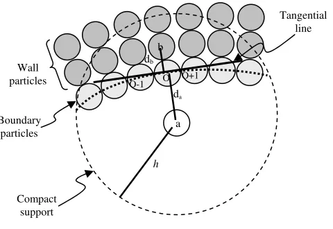
The velocity extrapolation method of Morris et al. [6] proved practical. According to this method, velocity of each fluid particle is extrapolated to neighbor wall particles (as an artificial velocity) across the tangent plane (or tangent line in 2D) of the boundary (Fig. 1). The unit vector of the tangent plane is i O i O i O i O i
x
x
x
x
t
1 1 1 1ˆ
− + − +−
−
=
. (28)In order to implement the aforementioned method for FSI problems, it can be assumed that there are ghost particles which have similar positions as wall particles. The artificial extrapolated velocity of each wall particle is attributed to the relevant ghost particle. Other properties of these ghost particles are similar to those of fluid particles.
(
)
(
i)
a i O b a i O i
b
u
d
d
u
u
u
ghost
=
+
−
, (29) [image:3.595.313.553.596.761.2]The no-slip boundary condition satisfies when velocity of ghost particles as well as boundary particles are contributed to calculate viscous forces.
Fig. 1 Boundary condition treatment to simulate no-slip boundary condition a b Compact support Wall particles Boundary particles Tangential line h
O-1 O O+1
da
T
t
=
0
.
4
T
t
=
0
.
2
T
t
=
0
.
8
T
[image:4.595.65.524.75.319.2]t
=
0
.
6
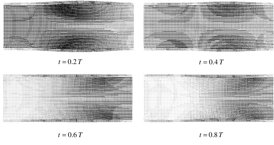
Fig. 2 Vector plot of velocity field at different stages of the flow pulse
VI. TEST CASE
The numerical test case is a two dimensional FSI simulation of a pulsatory flow moving through flexible walls. It is consisted of two flexible walls which are fixed at both ends with a length 0.09 m , a constant thickness
=
0
h
0.003m, a radiusR
0=
0.015m, and shear module ofG
=
1.5Mpa
. An incompressible viscous fluid, with densityρ
=
1000kg
m
3 and dynamic viscosity=
µ
0.004kg
m
s
; moving inside the constructed duct with a pulsatile flow volume rate of periodT
. The time dependent velocity, which is imposed at upstream, is taken to beT
t
B
A
t
U
(
)
=
+
sin
2
π
, (30)where
A
andB
are constant parameters which are selected to be 0.006 and 0.007 respectively. No-slip boundary condition is imposed on deformable walls. Square particles are selected with initial particle spacing of∆
x
f=
0.001m
and
∆
x
w=
∆
x
f2
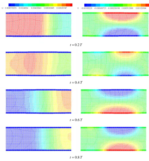
for fluids and solids respectively. Simulation needs several complete flow pulses to become stable. The vector plot of velocity field as well as its staggered plot is shown in Fig. 2 and Fig. 3 respectively at different stages of the pulse.VII. CONCLUSION
In this paper, a monolithic method for FSI problems involving no-slip boundary condition and internal fluid flows is developed using SPH. In order to improve the overall efficiency of the method, divergence of shear stress tensor for
fluids is substituted with the expression which was proposed by Morris et al. [6]. Moreover, the problem of dealing with moving boundaries to impose no-slip boundary condition is investigated using ghost particles which carry the extrapolated velocity.
VIII. REFERENCE
[1] K. Liu, H. Radhakrishnan, V. H. Barocas, “Simulation of flow around a thin, flexible obstruction by means of a deforming grid overlapping a fixed grid,” Int. J. Numer. Meth. Fluids, vol. 56, pp. 723-738, 2008. [2] R. van Loon, P. D. Anderson, J. de Hart, F. P. T. Baaijens, “A
combined fictitious domain/adaptive meshing method for fluid– structure interaction in heart valves,” Int. J. Numer. Meth. Fluids, vol. 46, pp. 533–544, 2004.
[3] C. Antoci, M. Gallati, S. Sibilla, “Numerical simulation of fluid– structure interaction by SPH,” Computers and Structures, vol. 85, pp. 879–890, 2007.
[4] S. M. Hosseini, N. Amanifard, “Presenting a modified SPH algorithm for numerical studies of fluid-structure interaction problems,” IJE Trans B: Applications, vol. 20, pp. 167-178, 2007.
[5] S. M. Hosseini, M. T. Manzari, S. K. Hannani, “A fully explicit three step SPH algorithm for simulation of non-Newtonian fluid flow, ” Int. J. of Numerical Methods for Heat and Fluid Flow, vol. 17, pp. 715– 735, 2007.
[6] J. P. Morris, P. J. Fox, Y. Zhu, “Modeling low Reynolds number incompressible flows using SPH,” J. Comp. Phys. Vol. 136, pp. 214– 226, 1997.
[7] J. Gray, J. J. Monaghan, R. P. Swift, “SPH elastic dynamics,”
Comput. Methods Appl. Mech. Eng. Vol. 190, pp. 6641–6662, 2001. [8] J. J. Monaghan, “Smoothed particle hydrodynamics,” Ann. Rev.
Astron. Astrophys. vol. 30, pp. 543–574, 1992.
[9] J. J. Monaghan, “Smoothed particle hydrodynamics,” Rep. Prog. Phys., vol. 68, pp. 1703–1759, 2005.
[10] J. L. Guermond, P. Minev, J. shen, “An overview of projection methods for incompressible flows,” Comput. Methods Appl. Mech. Engrg. vol. 195, pp. 6011-6045, 2006.
[11] D. Violeau, R. Issa, “Numerical modelling of complex turbulent free-surface flows with the SPH method: an overview,” Int. J. Numer. Meth. Fluids, vol. 53, pp. 277–304, 2007.
[13] L. D. Libersky, A. G. Petschek, T. C. Carney, J. R. Hipp, F. A. Allahdadi, “High strain Lagrangian hydrodynamics,” J. Comput. Phys. vol. 109, pp. 67-75, 1993.