Full Terms & Conditions of access and use can be found at
http://www.tandfonline.com/action/journalInformation?journalCode=rquf20
Download by: [Centrum Wiskunde & Informatica] Date: 20 April 2017, At: 04:17
Quantitative Finance
ISSN: 1469-7688 (Print) 1469-7696 (Online) Journal homepage: http://www.tandfonline.com/loi/rquf20
On an efficient multiple time step Monte Carlo
simulation of the SABR model
Álvaro Leitao, Lech A. Grzelak & Cornelis W. Oosterlee
To cite this article: Álvaro Leitao, Lech A. Grzelak & Cornelis W. Oosterlee (2017): On an efficient multiple time step Monte Carlo simulation of the SABR model, Quantitative Finance, DOI: 10.1080/14697688.2017.1301676
To link to this article: http://dx.doi.org/10.1080/14697688.2017.1301676
© 2017 The Author(s). Published by Informa UK Limited, trading as Taylor & Francis Group
Published online: 10 Apr 2017.
Submit your article to this journal
Article views: 40
View related articles
On an efficient multiple time step Monte Carlo
simulation of the SABR model
ÁLVARO LEITAO
∗†‡, LECH A. GRZELAK†§
and CORNELIS W. OOSTERLEE†‡
†TU Delft, Delft Institute of Applied Mathematics, Delft, The Netherlands
‡Centrum Wiskunde & Informatica (CWI), Amsterdam, The Netherlands
§ING, Quantitative Analytics, Amsterdam, The Netherlands
(Received 13 April 2016; accepted 24 February 2017; published online 10 April 2017)
In this paper, we will present a multiple time step Monte Carlo simulation technique for pricing options under theStochastic Alpha Beta Rhomodel. The proposed method is an extension of the one time step Monte Carlo method that we proposed in an accompanying paper Leitaoet al.[Appl. Math. Comput. 2017,293, 461–479], for pricing European options in the context of the model calibration. A highly efficient method results, with many very interesting and nontrivial components, like Fourier inversion for the sum of log-normals, stochastic collocation, Gumbel copula, correlation approximation, that are not yet seen in combination within a Monte Carlo simulation. The present multiple time step Monte Carlo method is especially useful for long-term options and for exotic options.
Keywords: SABR model; Exact simulation; Monte Carlo methods; Copulas; Stochastic collocation; Fourier techniques; Exotic options
JEL Classification: C15, C63
1. Introduction
The Stochastic Alpha Beta Rho (SABR) model (Haganet al.
2002) is an established stochastic differential equation (SDE) model which, in practice, is often used for interest rates and foreign-exchange (FX) modelling. It is based on a parametric local volatility component in terms of a model parameter,β, and reads
dS(t)=σ (t)Sβ(t)dWS(t), S(0)=S0exp(r T) ,
dσ (t)=ασ (t)dWσ(t), σ (0)=σ0.
(1) Here,S(t)= ¯S(t)exp(r(T −t))denotes the forward price of the underlying asset S¯(t), withr an interest rate, S0the spot
price andT the maturity. Further,σ (t)represents a stochastic volatility process, withσ (0)=σ0,WS(t)andWσ(t)are
corre-lated Brownian motions with constant correlation coefficient
ρ (i.e. WSWσ = ρt). The parameters of the SABR model
are α > 0 (the volatility of volatility,vol-vol), 0 ≤ β ≤ 1 (the variance elasticity) and ρ (the correlation coefficient). Because of a practically very useful closed-form expression for the implied volatility,Haganet al.(2002) andObloj(2008), the model has gained its popularity. However, since this expression is derived by perturbation theory, the formula is not always accurate for small strike values or for long time to maturity. By the one time step SABR method inLeitaoet al.(2017), we
∗Corresponding author. Email:[email protected]
can efficiently calculate accurate implied volatilities for any strike, however, only for short times to maturity (less than two years). This fits well to the context of FX markets.
Here, we extend the one time step Monte Carlo method from Leitaoet al. (2017), and propose a multiple time step Monte Carlo simulation techniquefor pricing options under the SABR dynamics. We call it themSABR method. With this new simulation approach, we can price options with longer maturities, payoffs relying on the transitional distributions and exotic options (like path-dependent options) under the SABR dynamics, overcoming the limitations of Hagan’s formula in the mentioned situations.
Because a robust and efficient SABR simulation scheme may be involved and quite expensive, we aim for using as few time steps as possible. This fact, together with the long-time horizon assumption, implies that we focus on larger long-time steps. In this context, the important research line is called
exact simulation, where, rather than Taylor-based simulation techniques, the probability density of the SDE under consider-ation is highly accurately approximated. Point-of-departure is Broadie and Kaya’s exact simulation for the Heston stochastic volatility model (Broadie and Kaya,2006). That method is, however, time-consuming because of multiple evaluations of Bessel functions and the use of Fourier inversion techniques on each Monte Carlo path. Inspired by this approach, inSmith (2007) andvan Hasstrecht and Pelsser(2010), computational
© 2017 The Author(s). Published by Informa UK Limited, trading as Taylor & Francis Group.
This is an Open Access article distributed under the terms of the Creative Commons Attribution-NonCommercial-NoDerivatives License (http://creativecommons.org/licenses/ by-nc-nd/4.0/), which permits non-commercial re-use, distribution, and reproduction in any medium, provided the original work is properly cited, and is not altered, transformed, or
improvements were proposed. Furthermore,Andersen(2008) presented two efficient alternatives to the Broadie and Kaya scheme, the so-called Truncated Gaussian and the Quadratic Exponential (QE) schemes.
For the SABR model, exact Monte Carlo simulation is non-trivial because the forward process in (1) is governed by
con-stant elasticity of variance (CEV) dynamics (Cox 1996,
Schroder 1989). InIslah(2009), the connection between the CEV and a squared Bessel processes was explained, and an analytic approximation for the SABR conditional distribution based on the non-centralχ2distribution was presented. The expression relies on the stochastic volatility dynamics, but also on theintegrated varianceprocess (which itself also depends on the volatility).
An (approximately) exact SABR simulation can then be subdivided in to the simulation of the volatility process, the simulation of the integrated variance (conditional on the volatil-ity process) and the simulation of the underlying CEV pro-cess (conditional on the volatility and the integrated variance processes). Based on this,Chenet al.(2012) proposed a low-biased Monte Carlo scheme with moment-matching (following the techniques of the QE scheme by Andersen (2008)) and a direct inversion approach. For the simulation of the inte-grated variance, they also employed moment-matching based on conditional moments that were approximated by a small disturbance expansion. InCaiet al.(forthcoming), the authors employed direct inversion for the forward distribution and used a Laplace transform inversion technique to simulate the integrated variance.Kennedy and Pham(2014) provided the moments of the integrated variance for specific SABR models (like the normal, log-normal and displaced diffusion SABR models) and derived an approximation of the SABR distribu-tion. InLord and Farebrother(2014), a summary of different approaches was presented.
In this work, we approximate the distribution of the inte-grated variance conditional on the volatility dynamics by join-ing the two involved marginal distributions, i.e. the stochastic volatility and integrated variance distributions, by means of copula techniques. With both marginal distributions available, we use the Archimedean Gumbel copula to define a multivari-ate distribution which approximmultivari-ates the conditional distribu-tion of the integrated variance given the stochastic volatility.
An approximation of the cumulative distribution function (CDF) of the integrated variance can be obtained by a recur-sive procedure, as described inZhang and Oosterlee(2013), originally employed to price arithmetic Asian options. This iterative technique is based on the derivation of the character-istic function of the integrated variance process and Fourier inversion to recover the probability density function (PDF).
The fact that we need to apply recursion and compute the corresponding characteristic function, PDF and CDF of the integrated variance for each Monte Carlo sample at each time step, makes this approach however computationally very ex-pensive (even with the improvements already made inLeitao
et al. (2017)), like the Heston exact simulation. In order to reduce the use of this procedure as much as possible, highly efficient sampling from the CDF of the integrated variance is proposed, which is based on the so-calledStochastic Colloca-tion Monte Carlo sampler(SCMC), seeGrzelaket al.(2015). The technique employs a sophisticated interpolation (based
on Lagrange polynomials and collocation points) of the CDF under consideration.
As will be seen, the resulting ‘almost exact’ Monte Carlo SABR simulation method that we present here (the mSABR method), contains several interesting (and not commonly used) components, like the Gumbel copula, a recursion plus Fourier inversion to approximate the CDF of the integrated variance and efficient interpolation by means of the SCMC sampler. The proposed mSABR scheme allows for fast and accurate option pricing under SABR dynamics, providing a better ratio of accuracy and computational cost than Taylor-based simulation schemes. Compared to the other approaches mentioned in this introduction, we provide a highly accurate SABR simulation scheme, based on only a few time steps.
The paper is organized as follows. In section2, SABR model simulation is introduced. In section3, the different parts of the multiple time step copula-based technique are described, including the derivation of the marginal distributions and the application of the copula. Some numerical experiments are pre-sented in section4. We conclude in section5. In the derivation of the CDF of the integrated variance, we need to perform sev-eral approximations, which comes with approximation errors. In appendix1, we list and discuss these errors.
2. ‘Almost exact’ SABR simulation
The SABR model with dependent Brownian motions was already given in (1). The multiple time step Monte Carlo SABR simulation is based on the corresponding SDE system with independent Brownian motions dWˆS(t)and dWˆσ(t), i.e.
dS(t)=σ (t)Sβ(t) ρdWˆσ(t)+ 1−ρ2dWˆ S(t) , S(0)=S0exp(r T) , dσ (t)=ασ (t)dWˆσ(t), σ (0)=σ0. (2)
The forward dynamics are governed by a CEV process. Based on this fact and the work bySchroder(1989) andIslah (2009), an analytic approximation for the CDF of the SABR conditional process has been obtained. For some generic time interval[s,t], 0≤s<t ≤T, assumingS(s) >0, the condi-tional cumulative distribution for forwardS(t)with an absorb-ing boundary atS(t)=0, givenσ (s),σ (t)andstσ2(z)dz, is given by Pr S(t)≤ K|S(s) >0, σ (s), σ (t), t s σ2(z) dz =1−χ2(a;b,c), (3) where a= 1 ν(t) S(s)1−β (1−β) + ρ α(σ (t)−σ (s)) 2 , c= K 2(1−β) (1−β)2ν(t), b=2−1−2β−ρ 2(1−β) (1−β)(1−ρ2) , ν(t)=(1−ρ2) t s σ2(z) dz,
This formula is exact in the case ofρ =0 and constitutes anapproximationotherwise (because the CEV process is ap-proximated by a shifted process with an apap-proximated initial condition for ρ = 0 in the derivation). Based on equation (3), an approximately exact simulation of SABR model is feasible by inverting the conditional SABR cumulative distri-bution when the conditional integrated variance is known, see section2.1.
2.1. SABR Monte Carlo simulation
In order to apply an ‘almost exact’ multiple time step Monte Carlo method for the SABR model, several steps need to be performed, that are described in the following:
• Simulation of the SABR volatility process, σ (t)given
σ (s). By equation (2), the stochastic volatility process of the SABR model exhibits a log-normal distribution. The solution is ageometric Brownian motion, i.e. the exact simulation ofσ (t)|σ (s)reads
σ (t)∼σ (s)exp αWˆσ(t)−1 2α 2t . (4) • Simulation of the SABR integrated variance process ,
t
s σ2(z)dz|σ (s), σ (t). This conditional distribution is
not available in closed form. We will therefore derive an approximation of the conditional distribution of the SABR integrated variance given σ (t) and σ (s). The integrated variance sampling can be done by simply inverting it.
• Simulation of the SABR forward price process.The for-ward priceS(t)can be simulated by inverting the CDF in equation (3). By this, we avoid negative forward prices in the simulation, as an absorbing boundary at zero is considered. There is no analytic expression for the inverse distribution and therefore this inversion has to be computed by means of some numerical approximation. The multiple time step Monte Carlo simulation for the SABR model is thus summarized in algorithm1. Input parameters are the initial conditions (S0 and σ0), the maturity time, T, the
SABR parameters α, β and ρ, the number of Monte Carlo samples (n) and the number of time steps (m).
Algorithm 1: Multiple time step SABR Monte Carlo simulation. Data:S0, σ0,T, α, β, ρ,n,m. S(0)=S0exp(r T),σ (0)=σ0 forPath p=1. . .ndo forStep k=1. . .mdo s=(k−1)Tm t=kmT Samplingσ (t)givenσ (s).
Samplingstσ2(z)dzgivenσ(s)andσ(t).
SamplingS(t)givenS(s),σ(s),σ(t)andstσ2(z)dz.
In section3.3, we propose a procedure to samplestσ2(z)dz|
σ (s), σ (t)based on the Gumbel copula. For this, the CDF of the integrated variance given the initial volatility, σ (s), (as a marginal distribution) must be derived. In section 3.1, a recursive technique to obtain an approximation of this CDF is
presented. Because we need to apply this recursion to approximate the characteristic function, the PDF and the CDF ofstσ2(z)dz|σ (s)for each sample ofσ (s)at each time step, this approach is expensive in terms of computational cost. To overcome this drawback, an efficient alternative will be employed here, based on Lagrange interpolation, as in the SCMC (Grzelaket al.,2015). In section2.2, this methodology is briefly described.
2.2. Stochastic collocation Monte Carlo sampler
In a multiple time step exact simulation Monte Carlo method we need to perform a significant number of computations each time step on each Monte Carlo path. This often hampers the applicability of the exact simulation for systems of SDEs. One of the important components of the multiple time step Monte Carlo SABR simulation is therefore an accurate and highly efficient interpolation, as proposed in the SCMC sampler in Grzelaket al.(2015).
In this section, we will introduce the SCMC technique. The details in the SABR conditional integrated variance context will be presented in section3.2.
The SCMC technique relies on the property that a CDF of a distribution (if it exists) is uniformly distributed. A well-known standard approach to sample from a given distribution,Y, with CDFFY reads
FY(Y) d
=U thus yn=FY−1(un),
where=d means equality in distributional sense,U ∼U([0,1]) andunare samples fromU([0,1]). The computational cost of
this approach highly depends on the cost of the inversionFY−1, which is assumed to be expensive.
We therefore consider another, ‘cheap’, random variableX, whose inversion, FX−1, is computationally much less expen-sive. In this framework, the following relation holds
FY(Y) d
=U =d FX(X).
The samplesynofY, andxnof X, are thus related via the
following inversion,
yn=FY−1(FX(xn)).
However, this does not yet imply any improvement since the number of expensive inversions FY−1remains the same. The goal is to compute yn using a functiong(·) = FY−1(FX(·)),
such that
FX(x)=FY(g(x)) and Y =d g(X),
where evaluations of function g(·) do not require many inversionsFY−1(·).
InGrzelaket al.(2015), functiong(·)is approximated by means of Lagrange interpolation, which is a well-known in-terpolation also used in the Uncertainty Quantification (UQ) context. The result is a polynomial, gNY(·), which approxi-mates functiong(·)=FY−1(FX(·)), and the samplesyncan be
yn≈gNY(xn)= NY i=1 yii(xn), i(xn)= NY j=1,j=i xn− ¯xj ¯ xi− ¯xj,
where xn is a vector of samples from X and x¯i andx¯j are
so-calledcollocation points.NY represents the number of
col-location points andyi the exact inversion value ofFY at the
collocation pointx¯i, i.e.yi = FY−1(FX(x¯i)). By applying this
interpolation, the number of inversions is reduced and, with onlyNY expensive inversionsFY−1(FX(x¯i)), we can generate
any number of samples by evaluating the polynomialgNY(xn). This constitutes the 1D version of SCMC sampler inGrzelak
et al.(2015).
According to the definition of the SCMC technique, a crucial aspect for the computational cost is parameter NY: the fewer
collocation points are required, the more efficient will be the sampling procedure. The collocation points must beoptimally
chosen in a way to minimize their number. For any random variableX, the optimal collocation points will be based on the moments ofX. The optimal collocation points are here chosen to be Gauss quadrature points that are defined as the zeros of the related orthogonal polynomial. This approach leads to a stable interpolation under the probability distribution of X. The complete procedure to compute the collocation points is described inGrzelaket al.(2015).
In section3.2, the application of SCMC technique to gen-erate samples from the CDF ofstσ2(z)dz|σ (s)is presented.
Since we deal with a conditional distribution, the 2D version of SCMC needs to be used.
3. Components of the mSABR method
In this section, we will discuss the different components of the mSABR method. For simplicity, hereafter, we denote the SABR’s integrated variance process byY(s,t):=stσ2(z)dz. We will explain how to efficiently sample the integrated vari-ance given the initial and the final volatility, i.e.Y(s,t)|σ (t),
σ (s), as well as its use in a complete SABR simulation. Since the distribution is not available in closed form, some approxi-mations need to be made. In section3.3, we propose an accurate sampling method based on copula theory (Sklar,1959), which is employed to approximate the required conditional distri-butions. The copula relies on the availability of themarginal
distributions to simulate thejointdistribution. As the marginal distributions,Y(s,t)|σ (s)andσ (t)|σ (s)appear as the natural choices. In section 3.1, a procedure to recover the CDF of the integrated variance process given the initial volatility is presented.
3.1. CDF ofstσ2(z)dz|σ (s)using the COS method
We present a technique to approximate the CDF of Y(s,t)|
σ (s), i.e. FY|σ(s). We will work in the log-space, so an
ap-proximated CDF of logY(s,t)|logσ (s), FlogY|logσ(s), will
be derived. We have employed this technique in the one time step SABR method (Leitaoet al.2017), but the multiple time step version is more involved. We approximateY(s,t)by its discrete equivalent, i.e.
Y(s,t):= t s σ 2(z)dz≈ M j=1 tσ2(tj)=: ˆY(s,t) (5)
whereMis the number of intermediate or discrete time points,†
t = t−Ms andtj =s+ jt, j =1, . . . ,M.Yˆ(T)is
subse-quently transformed to the logarithmic domain, with
FlogYˆ|logσ(s)(x)=
x
−∞ flogYˆ|logσ(s)(y)dy, (6)
and flogYˆ|logσ(s)the PDF of logYˆ(s,t)|logσ (s).
Density flogYˆ|logσ(s)is, in turn, found by approximating the associated characteristic function,φlogYˆ|logσ(s), and applying a Fourier inversion procedure. The characteristic function and the desired PDF of logYˆ(T)|logσ (s)form a Fourier pair. Based on the work inBenhamou(2002) andZhang and Oost-erlee(2013), we can define a recursive procedure to recover the characteristic function of flogYˆ|logσ(s).
3.1.1. Recursive procedure to recover φlogYˆ|logσ(s). We start by defining the sequence,
Rj =log σ2(t j) σ2(t j−1) , j =1, . . . ,M, (7) where Rj is the logarithmic increment of σ2(t)between tj
and tj−1, j = 1, . . . ,M. As the volatility process follows
log-normal dynamics, and increments of Brownian motion are independent and identically distributed, the Rj are also
inde-pendent and identically distributed, i.e. Rj d
= R. In addition, the characteristic function ofRjis well known and reads,∀u,j,
φRj(u)=φR(u)=exp(−i uα 2t−
2u2α2t), (8) withα as in (1) and i = √−1 the imaginary unit. By the definition ofRj in equation (7), we writeσ2(tj)as
σ2(t
j)=σ2(t0)exp(R1+R2+ · · · +Rj). (9)
At this point, a backward recursion procedure in terms ofRj
will be defined by which we can recoverφlogYˆ|logσ(s)(u). We define
Y1=RM, Yj =RM+1−j +Zj−1, j =2, . . . ,M.
(10) withZj =log(1+exp(Yj)).
By equations (9) and (10), the discrete integrated variance can be expressed as follows:
ˆ Y(s,t)= M i=1 σ2(t i)t =tσ2(s)exp(YM). (11)
From equation (11) and by applying the definition of char-acteristic function, we determineφlogYˆ|logσ(s), as follows:
†So, we have themlarge time steps, for the multiple time step Monte Carlo simulation, and we haveMintermediate dates for the integrated variance,M >>m. We suggest to prescribet, and useM= t−ts, in order to avoid over-discretization issues. This makes the value of Mdependent on the interval size,t−s.
φlogYˆ|logσ(s)(u)
=E[exp(i ulogYˆ(s,t))|logσ (s)]
=exp i ulog(tσ2(s)) E[exp(i uYM)|logσ (s)] =exp i ulog(tσ2(s)) φYM(u). (12) We have reduced the computation of φlogYˆ|logσ(s) to the computation ofφYM.AsYMis defined recursively, its character-istic function can be obtained by a recursion as well. According to the definition of the (backward) sequence Yj in equation
(10), the initial and recursive characteristic functions are given by the following expressions,
φY1(u)=φRM(u)=φR(u)=exp(−i uα 2t−
2u2α2t),
φYj(u)=φRM+1−j(u)φZj−1(u)=φR(u)φZj−1(u),
(13) where equation (8) is used in both expressions and the indepen-dence of RM+1−j andZj−1is also employed. By definition,
the characteristic function ofZj−1reads
φZj−1(u):=
∞
−∞(exp(x)+1) i uf
Yj−1(x)dx.
PDF fYj−1 is not known. To approximate it, the Fourier
cosine series expansion on fYj−1 is applied. We first truncate
the integration range to[a,b]. The calculation of integration boundaries a andb follows the cumulant-based approach as described inZhang and Oosterlee(2013) andFang and Oost-erlee(2008). After truncation of the integral and by applying a cosine series expansion to fYj−1, we have
φZj−1(u)≈ 2 b−a N−1 l=0 Bl b a (exp(x)+1)i u ×cos (x−a) lπ b−a dx=: ˆφZj−1(u), Bl = ˆ φYj−1 lπ b−a exp −i a lπ b−a , (14) withN the number of cosine expansion elements, and where
ˆ φY1(u):=φR(u), ˆ φYj(u):=φR(u)φˆZj−1(u). We wish to computeφˆYM( kπ b−a), fork=0, . . . ,N−1.
Con-sidering equation (14), we rewriteφˆYj(u)= φR(u)φˆZj−1(u)
in matrix–vector form, as follows:
j−1=MAj−1, (15) where j−1= j−1(k) N−1 k=0 , j−1(k)= ˆφZj−1(uk), M=[M(k,l)]kN=−01, M(k,l)= b a (exp(x)+1)iukcos((x−a)u l)dx, Aj = 2 b−a Aj(l) N−1 l=0 , Aj(l)= ˆ φYj−1(ul)exp(−i aul) , (16) with uz = zπ b−a. (17)
By the recursion procedure in equation (15), we obtain the approximationφˆYM of the characteristic functionφYM ofYM. 3.1.2. Numerical approximation of integral. For the approximation in equation (15), we must compute matrixM in equation (16) highly efficiently. The fast computation of the integral occurring for each element ofMis a key aspect for the performance of the mSABR method. The number of elements in matrixMcan be large, as it corresponds to the number of elements in the cosine series expansion, i.e. N2. The efficiency also depends on the required accuracy. In this work, we take advantage of the performed analysis inLeitao
et al.(2017). Among several options, the authors have shown that a numerical approximation based on a piecewise linear
approximationprovides a good balance between performance
and accuracy. Following this approximation, we rewrite the considered integral as follows:
IM:=
b
a
exp(i ukh(x))cos((x−a)ul)dx,
h(x)=log((exp(x)+1)), (18)
withukandulas in (17). Although functionh(x)is not linear,
it is smooth and monotonic (see figure1). Hence, the proposed numerical technique is to define sub-intervals of the integration range[a,b]in whichh(x)is almost constant or linear, i.e.
IM= L j=1 bj aj exp(i ukh(x))cos((x−a)ul)dx,
so that we can perform a first-order expansion in each sub-interval[aj,bj], j = 1, . . . ,L. In order to guarantee
conti-nuity of the approximation,h(x)is approximated by a linear function in each interval as follows:
h(x)≈c1,j+c2,jx, x ∈ [aj,bj].
This gives us an approximationIˆM, as follows ˆ IM= L j=1 exp(i ukc1,j) bj aj exp(i ukc2,jx)cos((x−a)ul)dx Ij . (19) In each sub-interval[aj,bj], we need to determine a simple
integral,Ij, which can be computed analytically.
The optimal integration pointsaj andbj in equation (19)
are found by differentiation ofh(x)w.r.t.x, i.e.
H(x):= ∂h(x) ∂x = exp(x) exp(x)+1 = 1 1+exp(−x),
giving a relation between the derivative ofh(x)and the logistic distribution. This representation indicates thatH(x)is the CDF of the logistic distribution, with a so-calledlocation parameter
μ=0 and ascale parameterη=1. In order to determine the optimal integration points so that their positions correspond to the logistic distribution, we need to compute the quantiles. The quantiles of the logistic distribution are analytically available and given by q(p)=log p 1−p .
The algorithm for the optimal integration points, given integration interval [a,b] and the number of intervals L, is then as follows:
• Determine an interval in the probability space: Ph = [H(a),H(b)].
• Divide the interval Ph equally into L parts: Phj = [pj,pj+1], j =0. . .L−1.
• Determineaj andbjby calculating the quantiles,aj =
q(pj)andbj =q(pj+1), j =0. . .L−1.
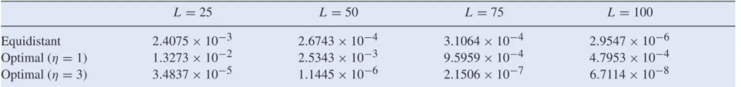
The algorithm above ensures that integration points are opti-mally distributed (see figure1(a)). However, for the particular problem, the integration interval can be rather large. As the integration points are typically concentrated near the function’s curved part, the errors in the outer sub-intervals dominate the overall error and more points at the beginning and at the end of the interval are required to reduce this error. A more evenly distribution of the integration points can be achieved by introducing a scale parameter,η = 1, which implies that the integration points correspond to a CDF with increased variance. In figure1(b), the case ofη=3 is presented. When
η=1, the expression for the quantiles reads,
q(p)=ηlog p 1−p .
Through the experiments inLeitaoet al.(2017), we concluded that the choiceη=3 provided accurate results in this context.
3.1.3. Recovering flogYˆ|logσ(s)by COS method. Once the approximation ofφYM,φˆYM, has been efficiently derived, we can recover flogYˆ|logσ(s)fromφlogYˆ|logσ(s)by employing the COS method (Fang and Oosterlee 2008), as follows:
flogYˆ|logσ(s)(x)≈ 2 ˆ b− ˆa N−1 k=0 Ckcos x− ˆa kπ ˆ b− ˆa , (20) with Ck = φlogYˆ|logσ(s) kπ ˆ b− ˆa exp −i akˆ π ˆ b− ˆa , and φlogYˆ|logσ(s) kπ ˆ b− ˆa =exp i kπ ˆ b− ˆalog tσ2(s) φYM kπ ˆ b− ˆa ≈exp i kπ ˆ b− ˆalog tσ2(s) ˆ φYM kπ ˆ b− ˆa ,
whereNis the number of COS terms,[ˆa,bˆ]is the support†of logYˆ(s,t)|logσ (s)and the primeandsymbols in equation (20) mean division of the first term in the summation by two and taking the real part of the complex-valued expressions in the brackets, respectively. CDFFlogYˆ|logσ(s) can be obtained by integration, plugging the approximated flogYˆ|logσ(s)from equation (20) into equation (6).
The characteristic function φlogYˆ|logσ(s) and PDF
flogYˆ|logσ(s) need to be derived for each sample of logσ (s)
†It can be calculated given the support ofYM,[a,b].
and this makes the computation of FlogYˆ|logσ(s) (and also its subsequent inversion) very expensive. In order to over-come this issue, the SCMC technique (see section2.2) will be employed approximating these rather expensive computations by means of an accurate interpolation.
3.2. Efficient sampling oflogYˆ|logσ (s)
By employing the SCMC technique, instead of directly com-putingFlogYˆ|logσ(s)for each sample of logσ (s), we only have to computeFlogYˆ|logσ(s)at the collocation points. In general, only a few collocation points are sufficient to obtain accu-rate approximations, which is a well-known fact from the UQ research field. This fact allows us to drastically reduce the computational cost of sampling the required distribution.
For the problem at hand, we require samples from the inte-grated variance conditional on the initial volatility, log
ˆ
Y(s,t)|logσ (s). Therefore, we need to make use of the2D
version of the SCMC technique. Two levels of collocation
points need to be chosen, one for each dimension. If we denote them by NYˆ and Nσ, respectively, the resulting number of inversions equals NYˆ ·Nσ. The formal definition of the 2D SCMC technique applied to our context reads
yn|vn ≈gNYˆ,Nσ(xn) = Nˆ Y i=1 Nσ j=1 F−1 logYˆ|logσ(s)=¯vj( FX(x¯i))i(xn)j(vn), (21)
where xnare the samples from X ∼N(0,1), which is used
as the cheap variable, andvnthe samples of logσ (s);x¯i and ¯
vjare the collocation points for approximating variables logY
and logσ (s), respectively. The Lagrange polynomialsi and
j are defined by i(xn)= NYˆ k=1,k=i xn− ¯xk ¯ xi − ¯xk, j(vn)= Nσ k=1,k=j vn− ¯vk ¯ vi− ¯vk.
The collocation pointsx¯iandv¯j are calculated based on the
moments of the random variables. The two involved variables in the application of the 2D SCMC technique are the colloca-tion variables, X ∼ N(0,1), and logσ (s) ∼ N(logσ0+
1 2α
2s, α√s). The moments of a normal variable, X ∼ N
(μX,sX)are analytically available, and are given by
EXp=
0 if pis odd,
sXp(p−1)!! if pis even,
where pis the moment order and the expression!!represents thedouble factorial. In order to compute the optimal colloca-tion points,v¯j, the precalculated collocation points by means
of the logσ (s)moments need to be shifted according to the mean, i.e. logσ0+12α2s.
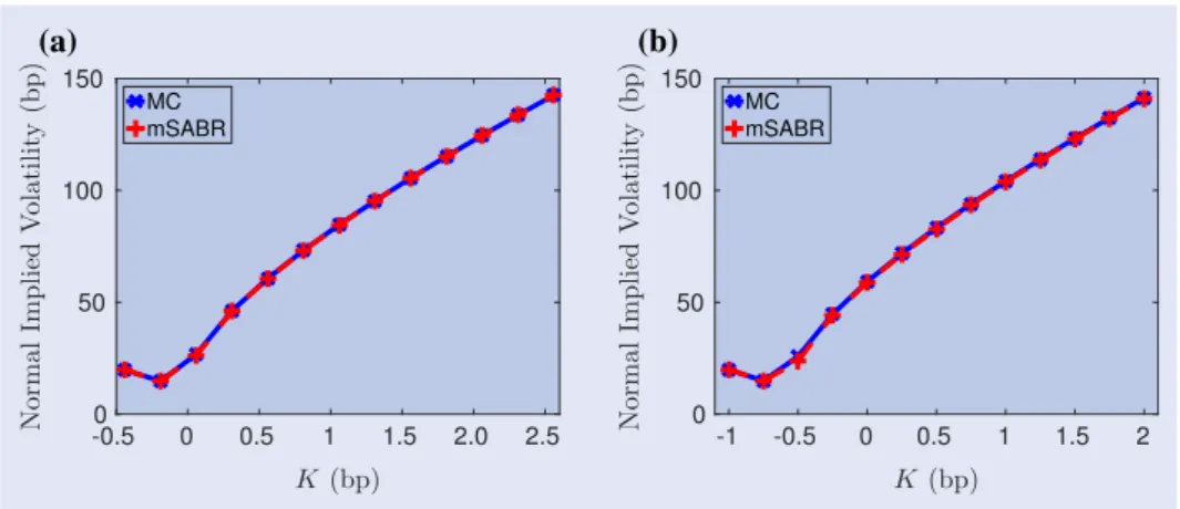
We first test numerically the accuracy of the SCMC tech-nique for our problem. In figure2, two experiments are pre-sented. In figure 2(a), we compare the samples obtained by direct inversion and by the SCMC technique. The fit is highly accurate, already with only seven collocation points. In figure 2(b), the empirical CDFs are depicted, where the excellent match is confirmed.
Figure 1. Optimal integration points.L=25.
Figure 2. (a) Points cloud logYˆ|logσ (s)by direct inversion (DI) sampling (red dots) and SCMC sampling (black circles). (b) Empirical CDFs of logY|logσ (s)with and without using SCMC.
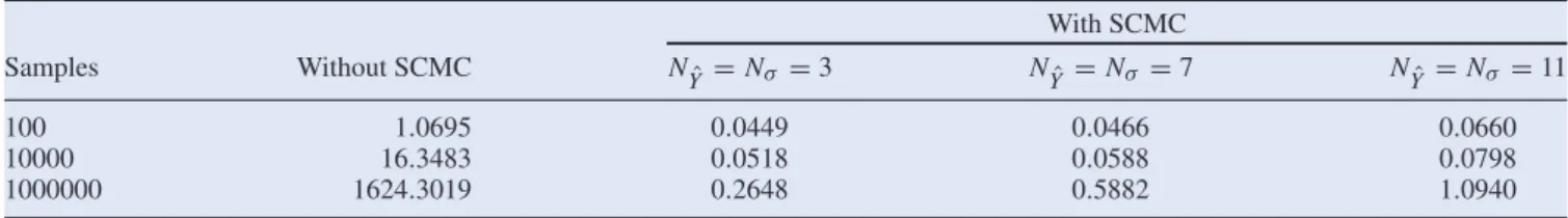
In order to show the performance of SCMC technique for the simulation of logYˆ|logσ (s), the execution times of generating different numbers of samples are presented in table1.
In appendix 1, the different sources of error due to the approximations made in the sections3.1and3.2are analysed.
3.3. Copula-based simulation ofstσ2(z)dz|σ (t), σ (s)
In this section, we present an algorithm for the simulation of the integrated variance given σ (t)and σ (s)by means of a copula. In order to obtain the joint distribution, we require the marginal distributions. In our case, the required CDFs are
FlogY|logσ(s)and Flogσ(t)|logσ(s). In section3.1, an
approxi-mated CDF of logY|logσ (s),FlogYˆ|logσ(s), has been derived. Since σ (t) follows a log-normal distribution, by definition, logσ (t)is normally distributed, and the conditional process logσ (t)given logσ (s), follows a normal distribution,
logσ (t)|logσ (s)∼N logσ (s)−1 2α 2(t−s), α√t−s . (22)
3.3.1. Pearson’s correlation coefficient. For any copula some measure of the correlation between the marginal dis-tributions is needed. We will employ the Pearson correlation coefficient for logY(s,t)and logσ (t). For this quantity, an approximated analytic formula can be derived. By definition, we have
PlogY,logσ(t) =corr log t s σ 2(z)dz,logσ (t) = cov logstσ2(z)dz,logσ (t) var
logstσ2(z)dzvar [logσ (t)]
Table 1. SCMC time in seconds. With SCMC Samples Without SCMC NYˆ =Nσ =3 NYˆ= Nσ =7 NYˆ =Nσ =11 100 1.0695 0.0449 0.0466 0.0660 10000 16.3483 0.0518 0.0588 0.0798 1000000 1624.3019 0.2648 0.5882 1.0940
We employ the following approximation
log t s σ2(z) dz≈ t s logσ2(z)dz=2 t s logσ (z)dz.
where the logarithm and the integral are interchanged. Since the log function is concave, this approximation forms a lower bound for the true value. This can be seen by applying Jensen’s inequality, i.e. log t s σ2(z)dz≥ t s logσ2(z)dz.
It has been numerically shown that, under the model settings with an interval sizet−sless than two years, the results based on this approximation are highly satisfactory (further details inLeitaoet al.(2017)). The correlation coefficient can then be approximated by
PlogY(T),logσ(t)≈
covstlogσ (z)dz,logσ (t)
varstlogσ (z)dz var [logσ (t)] .
To compute the covariance, we need E stlogσ (z)dz
logσ (t)
,Estlogσ (z)dz
andE[logσ (t)]. From equation (4), the last expectation as well as var [logσ (t)] are known. We find that logσ (t)=logσ0− 1 2α 2t+αW(t)=:η(t)+αW(t), and t s logσ (z)dz =logσ0(t−s)− 1 4α 2(t2−s2)+α t s W(z)dz =:γ (s,t)+α t W(t)−sW(s)− t s zdW(z) .
Based on these equations, using
E[logσ (T)]=η(t), E t s logσ (z)dz =γ (s,t),
we obtain the following expressions for the remaining expectation, E t s logσ (z)dz logσ (t) =E γ (s,t)+α t W(t)−sW(s)− t s zdW(z) ×(η(t)+αW(t))] =η(t)γ (s,t)+α2 t2−s2−E t s zdW2(z) =η(t)γ (s,t)+1 2α 2(t2−s2).
For the variance ofstlogσ (z)dz, we first compute E t s logσ (z)dz 2 =E γ (s,t)+α t W(t)−sW(s)− t s zdW(z) 2 =γ2(s,t)+α2E(t W(t)−sW(s))2 +α2E t s zdW(z) 2 −2α2E (t W(t)−sW(s)) t s zdW(z) , where E(t W(t)−sW(s))2 =t2E (W(t))2 +s2E (W(s))2 −2stE[W(s)W(t)] =t3+s3−2s2t, E t s zdW(z) 2 = t s z2dz=1 3(t 3−s3), E (t W(t)−sW(s)) t s zdW(z) =tE W(t) t s zdW(z) −sE W(s) t s zdW(z) =tE t s dW(z) t s zdW(z) −sE s s dW(z) t s zdW(z) =1 2t(t 2−s2),
and the variance reads var t s logσ (z)dz =E t s logσ (z)dz 2 − E t s logσ (z)dz 2 =α2 t3+s3−2s2t+1 3(t 3−s3)−t(t2−s2) =α2 1 3t 3+2 3s 3−s2t .
An approximation of the Pearson correlation coefficient is then obtained as follows:
PlogY,logσ(t)≈ η(t)γ (s,t)+12α2(t2−s2)−η(t)γ (s,t) α21 3t3+ 2 3s3−s2t α2t = t2−s2 213t4+2 3ts3−t2s2 . (23) Some copulas do not employ, in their definition, Pearson’s coefficient as the correlation measure. For example, Archimedean copulas employ the Kendall’sτrank correlation coefficient. However, a relation between both Pearson’s and Kendall’sτ coefficients is available,
P=sin π
2τ
.
3.3.2. Gumbel copula. In this work, we will use Archimedean Gumbel copula. The Gaussian copula may seem a natural choice, asσ (t)follows a log-normal distribution and
Y(T) = stσ2(z)dz can be seen as summation of squared log-normal processes. However, in Leitao et al.(2017), we have empirically shown that the Gumbel copula performs most accurately in this context for a variety of SABR parameter val-ues. The formal definition of the Archimedean Gumbel copula, consideringF1. . . ,Fd ∈ [0,1]das the marginal distributions,
reads Cθ(F1. . . ,Fd)=exp ⎛ ⎝− d i=1 (−log(Fi))θ 1/θ⎞ ⎠, (24)
where(−log(·))θ,θ >0 is the so-calledgenerator functionof the Gumbel copula. In order to calibrate parameterθ, a relation betweenθand the rank correlation coefficient Kendall’sτcan be employed, i.e.θ =1/(1−τ).
So, we have derived approximations for all the components required to apply the copula-based technique for the integrated variance simulation. The algorithm to samplestσ2(z)dzgiven
σ (t)andσ (s)then consists of the following steps: (1) Determine Flogσ(t)|logσ(s)by equation (22).
(2) Determine FlogYˆ|logσ(s)by equation (6).
(3) Determine the correlation between logY(s,t) and logσ (t)by equation (23).
(4) Generate correlated uniform samples,Ulogσ(t)|logσ(s)
andUlogYˆ|logσ(s)from the Gumbel copula by equation (24).
(5) FromUlogσ(t)|logσ(s), invert the CDFFlogσ(t)|logσ(s)
to get the samples σ˜n of logσ (t)|logσ (s). This
procedure is straightforward since the normal distri-bution inversion is analytically available.
(6) From UlogYˆ|logσ(s), invert the CDF FlogYˆ|logσ (s) to get the samplesy˜n of logYˆ|logσ (s). We propose an
inversion procedure based on linear interpolation. First, we evaluate the CDF function at some discrete points. Then, the insight is that, by rotating the CDF under consideration, we can interpolate over probabilities. This is possible when the CDF function is a smoothly increasing function. The interpolation polynomial pro-vides the quantiles of the original distribution from some given probabilities. SinceFlogYˆ|logσ(s)is indeed a smooth and increasing function, the interpolation-based inversion is definitely applicable. This procedure together with the use of 2D SCMC sampler (see section 3.2) results in a fast and accurate inversion.
(7) The samples σn of σ (t)|σ (s) and yn of Y(s,t) = t
s σ2(z)dz|σ (t), σ (s)are obtained by simply taking
exponentials as follows:
σn=exp(σ˜n), yn=exp(y˜n).
3.4. Simulation ofS(t)givenS(s),σ (s),σ (t)andstσ2(z)dz
We complete the mSABR method by the conditional sampling of S(t). The most commonly used techniques can be classi-fied in two categories: direct inversion of the SABR distri-bution function given in equation (3) and moment-matching approaches. The direct inversion procedure has a higher com-putational cost because of the evaluation of the non-central
χ2 distribution. However, some recent developments make
this computation affordable. Chen et al. (2012) proposed a forward asset simulation based on a combination of moment-matching (Quadratic Gaussian) and enhanced direct inversion procedures. We employ this technique also here. Note how-ever that, for some specific values ofβ, the simulation of the conditionalS(t)givenS(s),σ (s),σ (t)andstσ2(z)dzenables analytic expressions.
3.4.1. Caseβ=0. Forβ=0, it is easily seen from equation (2) that the asset process (in integral form) becomes
S(t)=S(s)+ρ t s σ ( z)dWˆσ(z)+ 1−ρ2 t s σ ( z)dWˆS(z). where t s σ (z)dWˆσ(z)= 1 α(σ (t)−σ (s)) , (25) and t s σ (z)dWˆS(z)|σ (t), σ (s)∼N ⎛ ⎝0, ! t s σ2(z)dz ⎞ ⎠. (26) Since this allows negative asset prices, the simulation ofS(t)
withβ =0 must be corrected. If the price at the initial time is less or equal to zero, i.e.S(s)≤0, the priceS(t)must remain zero for all time. Otherwise,
S(t)=max(S(t),0).
This correction is performed to be consistent within the whole simulation procedure, since the distribution of the ‘exact’SABR
simulation in equation (3) relies on the conditionS(s) > 0. If negative values are permitted, this must be handled in a different way (seeHaganet al.(2014) orAntonovet al.(2015), for example).
3.4.2. Caseβ=1. In the case ofβ =1, the asset dynamics in equation (1) become log-normal and the solution is given by S(t)=S(s)exp −1 2 t s σ2(z) dz+ρ t s σ (z)dWˆσ(z) +(1−ρ2) t s σ (z)dWˆS(z) .
If we take the log-transform, log S(t) S(s) = −1 2 t s σ2(z) dz+ρ t s σ (z)dWˆσ(z) +(1−ρ2) t s σ (z)dWˆS(z),
and by considering again equations (25) and (26), we obtain the distribution of log
S(t) S(s) |t s σ2(z)dz, σ (t), σ (s), which reads N −1 2 t s σ 2(z)dz+ρ α(σ (t)−σ (s)) , × ! (1−ρ2) t s σ2(z)dz ⎞ ⎠. (27)
By employing equation (27), the asset dynamicsS(t)can be sampled from S(t)∼S(s)exp −1 2 t s σ 2(z)dz+ρ α(σ (t)−σ (s)) +X ! (1−ρ2) t s σ2(z)dz ⎞ ⎠, (28)
where Xis the standard normal.
3.4.3. Case β = 0,β = 1. As mentioned before, for the generic case ofβ ∈ (0,1), we employ the enhanced inver-sion of the SABR asset price distribution in equation (3) as introduced inChenet al. (2012). We briefly summarize this approach. The asset simulation is performed either by a moment-matched quadratic Gaussian approximation or by an enhanced direct inversion. The authors inChenet al.(2012) proposed a threshold value to choose the suitable technique among these two. The moment-matching approach relies on the fact that, forS(s)0, the distribution function in equation (3) can be approximated by Pr S(t)≤K|S(s) >0, σ (s), σ (t), t s σ2(z) dz ≈χ2(c; 2−b,a).
By definition, the mean,μand the variance,κ2, of a generic
non-central chi-square distributionχ2(x;δ, λ)areμ:=δ+λ andκ2:=2(δ+2λ), respectively. A variableZ ∼χ2(x;δ, λ)
is accurately approximated by a quadratic Gaussian distribu-tion, as follows Z ≈d d(e+X)2, X∼N(0,1), with ψ:= μκ22, e2=2ψ−1−1+ 2ψ−1 2ψ−1−1≥0, d = μ 1+e2.
Applying this to the case in equation (3), we can sample the conditional asset dynamics, 0≤s<t, by
S(t)= (1−β)2(1−ρ2)d(e+X)2 t s σ2(z)dz 1 2(1−β) .
The moment-matching approximation is safely and accurately applicable when 0< ψ ≤ 2 andμ ≥ 0 (Chenet al.2012). Otherwise, a direct inversion procedure must be employed. A root-finding Newton method is then used. In order to reduce the number of Newton iterations (and the expensive evalu-ation of the non-central chi-square CDF), the first iterevalu-ations are based on an approximated formula for the non-central chi-square distribution, which is based on the normal CDF and derived bySankaran(1963). Then, the obtained value is employed as the initial guess for the Newton algorithm. The result is a significant reduction in the number of iterations and, hence, in the computational cost. Furthermore, this root-finding procedure consists of only basic operations, so that the whole procedure can be easily vectorized, leading to a further efficiency improvement.
As in the case ofβ = 0, the absorbing boundary at zero needs to be prescribed to avoid negative prices.
The resulting sampling procedure is robust and efficient.
3.4.4. Martingale correction. As already pointed by Andersen (2008) and Chen et al. (2012), the almost exact simulation of the asset price in some stochastic volatility mod-els can produce a loss of the martingale property, due to the approximation of a continuous process by its discrete equiv-alent. This is especially seen, when the size of time step is large and for certain configurations of the SABR parameters, like smallβ values, close-to-zero initial asset valuesS0, high
vol-vol parameterα or large initial volatilityσ0. In order to
overcome this issue, we incorporate to the mSABR method the use of a simple but effective numerical martingale correction, as follows: S(t)=S(t)−1 n n i=1 Si(t)+E[S(t)], =S(t)−1 n n i=1 Si(t)+S0,
where Si(t)represents thei−th Monte Carlo sample. Note,
however, that, for practical SABR parameters, the martingale error is very small and can be easily controlled by increasing the number of overall time stepsm.
4. Numerical experiments
In this section, we benchmark the mSABR method by pricing options under the SABR dynamics. We will consider several parameter configurations, extracted from the literature (see table 2), a zero-correlation set as in Grzelak et al. (2015) (set I), a set under log-normal dynamics as inChenet al.(2012) (set II), a medium long time to maturity set as in Antonov
et al.(2013) (set III) and a more extreme set as in Antonov
et al.(2015) (set IV). The strikes,Ki, are chosen following the
expression
Ki(T)=S(0)exp(0.1×T ×δi),
δ= {−1.5,−1.0,−0.5,0.0,0.5,1.0,1.5}, introduced byPiterbarg(2005).
Other parameters include:
• Step size in equation (5):t =5×10⁻⁵.
• Number of terms in equations (14) and (20):N =150. • Number of intervals for piecewise linear approximation
in equation (19):L=100.
• Number of collocation points in equation (21): NYˆ = Nσ =3.
• Number of samples:n=1.000.000.
The experiments were performed on a computer with CPU Intel Core i7-4720HQ 2.6 GHz and RAM memory of 16 Gigabytes. The employed software package was Matlab r2015b.
As usual, the European option prices are obtained by averag-ing the maximum of the forward asset values at maturity minus the strike and zero, i.e. max(S(T)−Ki(T),0)(call option).
Subsequently, the Black–Scholes formula is inverted to deter-mine theimplied volatilities. Note that, once the forward asset is simulated by the mSABR method, we can price options at multiple strikes simultaneously.
4.1. Convergence test
We perform a convergence study in terms of the number of time steps,mand, subsequently, in terms of the number of samples,
n. Set I is considered suitable for this experiment, since an analytic solution is available byAntonovet al.(2013) when
ρ=0, and it can be used as a reference. Also, as equation (3) is employed to sample the forward asset dynamics, the case
ρ=0 results in anexact simulation.
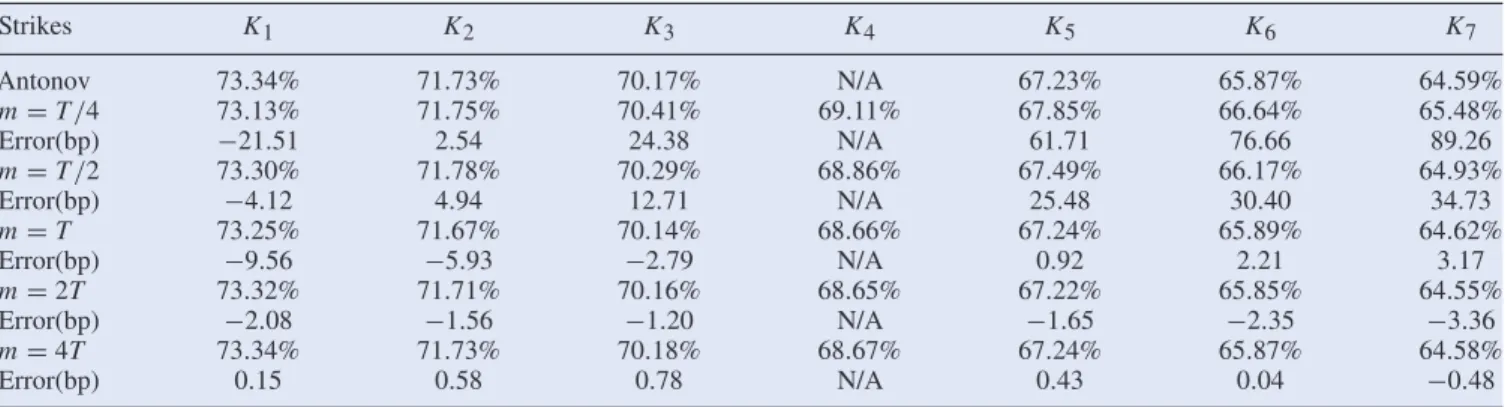
In table3, the implied volatilities obtained by the mSABR method for several choices of the number of time stepsmare presented. We observe by the errors in basis points (bp) that, by increasing the number of time steps, the technique converges very rapidly. Furthermore, only a few time steps are required to obtain accurate results: with only m = 4 time steps (one per year) the error is already less than ten basis points and withm = 4T (the time step size is a quarter of year), the error remains below one basis points. Compared to the low-bias SABR simulation schemeproposed inChenet al.(2012), the mSABR method is more accurate, since it relies on the
exact simulation of the integrated variance, whereas the low-bias scheme approximates the integrated variance by a small disturbance expansion and moment-matching techniques. That scheme performs worse when bigger time steps are considered.
We also perform a convergence test in the number of samples, n. According to the previous experiment and in order to guarantee that the errors do not increase by the time discretization, we setm=4T. In table4, the implied volatili-ties for increasingnare presented. By therelative error(RE), we can see that, as expected, the error is approximately reduced by a factor of 1/√n. Furthermore, we wish to show how the number of samples affects the variance of the mSABR method. In figure 3, the standard deviations† for several choices of
n are presented. Two strikes are evaluated, onein-the-money
strike, K2, and oneout-of-the-moneystrike,‡ K6. An
identi-cal behaviour can be observed for all other strikes as well. Again, we see a fast convergence and variance reduction in terms ofn.
4.2. Performance test
Next to the convergence of the mSABR method in terms of
mandn, another important aspect is the computational cost. Specifically, we will measure the execution times of an option pricing experiment using different alternative Monte Carlo-based methods and compare them with the mSABR method. Again, parameter Set I is employed since a reference value is available for this case. We consider a plain Monte Carlo Euler (MC Euler) discretization scheme for the forward asset,S(t). Note that the absorbing boundary at zero must be handled with care. Since our main contribution here is the exact simulation of the integrated variance, it is natural to also compare the performance with other, less involved, techniques. We there-fore also present a comparison between the mSABR method and two techniques where the integrated variance is either approximated bystσ2(z)dz≈σ2(s)(t−s)(left rectangular rule) orstσ2(z)dz ≈ 12(σ2(t)+σ2(s))(t−s)(trapezoidal rule). We denote these alternatives as the Y -Euler and Y -trpzschemes, respectively. The simulation ofS(t)is, in both cases, carried out as explained in section3.4. In table5, we present execution times (in seconds) of the MC Euler,Y -Euler,
Y -trpz and mSABR schemes, to achieve a certain level of
accuracy (measured as the error of the implied volatilities in basis points). In addition, the required number of time steps is presented in parentheses to provide an insight in the efficiency. Furthermore, the speedup obtained by our method is included in table6. We observe that the mSABR method is superior in terms of the ratio between computational cost and accuracy. The accuracy ofY-Euler orY-trpz can be improved by adding intermediate time steps, but then also the computational cost increases.
4.3. ‘Almost exact’ SABR simulation by varyingρ
As a next experiment we test the stability of the mSABR method when correlation parameter ρ varies from negative to positive values. As stated before, equation (3) is only exact forρ = 0. For that, we use Set II since the conditional for-ward asset simulation enables a closed-form solution (given by equation (28)) forβ =1. The considered values areρ = {−0.5,0.0,0.5}. Following the outcome of the previous exper-iment, we setm =4T. As a reference, a Monte Carlo (MC) †Computed by performing 100 realizations.
Table 2. Data sets.
S0 σ0 α β ρ T
Set I (Grzelaket al.2015) 0.5 0.5 0.4 0.5 0.0 4 Set II (Chenet al.2012) 0.04 0.2 0.3 1.0 −0.5 5 Set III (Antonovet al.2013) 1.0 0.25 0.3 0.6 −0.5 20 Set IV (Antonovet al.2015) 0.0056 0.011 1.080 0.167 0.999 1
Table 3. Implied volatility, increasingm: Antonov vs. mSABR. Set I.
Strikes K1 K2 K3 K4 K5 K6 K7 Antonov 73.34% 71.73% 70.17% N/A 67.23% 65.87% 64.59% m=T/4 73.13% 71.75% 70.41% 69.11% 67.85% 66.64% 65.48% Error(bp) −21.51 2.54 24.38 N/A 61.71 76.66 89.26 m=T/2 73.30% 71.78% 70.29% 68.86% 67.49% 66.17% 64.93% Error(bp) −4.12 4.94 12.71 N/A 25.48 30.40 34.73 m=T 73.25% 71.67% 70.14% 68.66% 67.24% 65.89% 64.62% Error(bp) −9.56 −5.93 −2.79 N/A 0.92 2.21 3.17 m=2T 73.32% 71.71% 70.16% 68.65% 67.22% 65.85% 64.55% Error(bp) −2.08 −1.56 −1.20 N/A −1.65 −2.35 −3.36 m=4T 73.34% 71.73% 70.18% 68.67% 67.24% 65.87% 64.58% Error(bp) 0.15 0.58 0.78 N/A 0.43 0.04 −0.48
Table 4. Implied volatility, increasingn: Antonov vs. mSABR. Set I.
Strikes K1 K2 K3 K4 K5 K6 K7 Antonov 73.34% 71.73% 70.17% N/A 67.23% 65.87% 64.59% n=102 67.29% 65.55% 63.84% 62.20% 60.63% 59.01% 57.65% RE 8.24×10⁻² 8.61×10⁻² 9.01×10⁻² N/A 9.82×10⁻² 1.04×10⁻¹ 1.07×10⁻¹ n=104 73.41% 71.87% 70.36% 68.91% 67.51% 66.19% 64.94% RE 9.65×10⁻⁴ 1.94×10⁻³ 2.75×10⁻³ N/A 4.08×10⁻³ 4.93×10⁻³ 5.48×10⁻³ n=106 73.34% 71.73% 70.18% 68.67% 67.24% 65.87% 64.58% RE 2.04×10⁻⁵ 8.08×10⁻⁵ 1.11×10⁻⁴ N/A 6.39×10⁻⁵ 6.07×10⁻⁶ 7.43×10⁻⁵
Figure 3. Convergence of the mSABR method.
simulation with a very fine Euler time discretization (1000T
time steps) in the forward asset process is employed. In table7, the resulting implied volatilities are provided. The differences between the Monte Carlo volatilities and the ones given by the mSABR method are within 10 basis points for all choices ofρ.
4.4. Pricing barrier options
We will price barrier options with the mSABR method. The
up-and-outcall option is considered here, with the barrier level,
B, B > S0,B > Ki. The price of this type of barrier option