Two spécific problems in Data Science: Demand forecasting using weather data and Non-linear causality inference

Unicentre

CH-1015 Lausanne http://serval.unil.ch

Year : 2019

Two spécific problems in Data Science: Demand forecasting

using weather data and Non-linear causality inference

Babongo Bosombo Flora

Babongo Bosombo Flora, 2019, Two spécific problems in Data Science: Demand forecasting using weather data and Non-linear causality inference

Originally published at : Thesis, University of Lausanne

Posted at the University of Lausanne Op

Document URN : urn:nbn:ch:serval-BIB_35E2A0F511042 Droits d’auteur

L'Université de Lausanne attire expressément l'attention des utilisateurs sur le fait que tous les documents publiés dans l'Archive SERVAL sont protégés par le droit d'auteur, conformément à la loi fédérale sur le droit d'auteur et les droits voisins (LDA). A ce titre, il est indispensable d'obtenir le consentement préalable de l'auteur et/ou de l’éditeur avant toute utilisation d'une oeuvre ou d'une partie d'une oeuvre ne relevant pas d'une utilisation à des fins personnelles au sens de la LDA (art. 19, al. 1 lettre a). A défaut, tout contrevenant s'expose aux sanctions prévues par cette loi. Nous déclinons toute responsabilité en la matière.

Copyright

The University of Lausanne expressly draws the attention of users to the fact that all documents published in the SERVAL Archive are protected by copyright in accordance with federal law on copyright and similar rights (LDA). Accordingly it is indispensable to obtain prior consent from the author and/or publisher before any use of a work or part of a work for purposes other than personal use within the meaning of LDA (art. 19, para. 1 letter a). Failure to do so will expose offenders to the sanctions laid down by this law. We accept no liability in this respect.

FACULTÉ DES HAUTES ÉTUDES COMMERCIALES DÉPARTEMENT DES SYSTÈMES D’INFORMATION

Two specific problems in Data Science: Demand forecasting using weather data

and

Non-linear causality inference

THÈSE DE DOCTORAT présentée à la

Faculté des Hautes Études Commerciales de l'Université de Lausanne

pour l’obtention du grade de

Docteure ès Sciences en systèmes d’information par

Flora BABONGO BOSOMBO

Directeur de thèse Prof. Ari-Pekka Hameri

Co-directrice de thèse Prof. Valérie Chavez-Demoulin

Jury

Prof. Felicitas Morhart, Présidente Prof. Olivier Gallay, expert interne Prof. Ralf Seifert, expert externe

THESIS COMMITTEE:

Ari-Pekka HAMERI

Thesis supervisor, Professor of Operations management, Faculty of Business and

Economics (HEC), University of Lausanne

Valérie CHAVEZ-DEMOULIN

Thesis co-supervisor, Professor of Statistics, Faculty of Business and Economics

(HEC), University of Lausanne

Felicitas MORHART

President of the jury, Professor of Marketing, Faculty of Business and Economics

(HEC), University of Lausanne

Olivier GALLAY

Internal expert, Professor of Statistics, Faculty of Business and Economics (HEC),

University of Lausanne

Ralf SEIFERT

External expert, Professor of Mathematical models in supply chain

management, Federal Polytechnic School of Lausanne EPFL

Dedication

I dedicate this thesis to all my family , especially

• To my elder sisterJudith BABONGOand her husbandPierrot MUNDEMBA • To my godparentsChristoph SOLANDandMarie-Françoise PIOT

their unconditional love and support have been an integral part of the comple-tion of this thesis, and I am eternally grateful for everything they have done for me.

Acknowledgement

First and foremost, I wish to thank my advisors, Ari-Pekka Hameri and Valérie Chavez-Demoulin, for their mentoring and trust. They offered me their helpful guidance and advice which helped me to grow further as an academic researcher and as a person.

A special thanks to Tapio Niemi, co-author in 3 of the papers developed in this thesis, for his comments and discussions that significantly contributed to improve my research.

I also would like to acknowledge my committee members for their time and expertise.

I am grateful to the University of Lausanne, which enabled me to work under perfect conditions. Additionally I want to thank the Swiss National Science Foundation for their financial support.

I thank all my friends and colleagues, members of the Department of Opera-tions and of the Department of Information Systems.

Finally I would like to thank my family, who has always been there to listen, support and encourage me. They were emotionally an infinite support.

Abstract

In this thesis, I investigate two specific subjects in data science, namely demand forecasting and causality inference, dividing this thesis in two main parts. The first part aims at improving demand forecasting accuracy that impacts supply chain performance. It consists of three articles aiming at studying how to enhance demand forecasting accuracy using pertinent data (e.g. operational transaction data, weather data, socio-economic data, etc.). Each article ex-plores a new statistical approach on the supply chain optimization through demand forecasting accuracy.

• In the first article we analyze transactional longitudinal data of several business units, matched with daily location-based weather conditions. We also study ways in which weather fluctuations affect supply chain performance though the delivery delay in days. Understanding this re-lationship is valuable both for improving sales forecast accuracy and for improving operational performance.

• The second article aims at explaining how weather conditions and fluc-tuations affect the accuracy of demand forecasting for seasonal products. We found that weather conditions have a significant impact on demand forecasting accuracy with reductions in percentage errors up to 45%. These results can be used to justify and motivate the integration of the impact of variability in weather in the decision making process in or-der to better anticipate demand volumes and reduce costs due to excess inventory or stock shortages.

• The goal of the third article is to improve demand forecasting accuracy by using the concept of spatial dependence and interpolation, and incor-porating the effects of socio-economic aspects and weather conditions in the spatial dependence structure. The accuracy of demand forecasting is improved, the reduction of the forecasting error is up to 48%.

The goal of the second part is to infer the causal relationship in the case of non-linearity and heteroscedasticity.

• In the fourth article, a two-steps method is proposed to infer the intrinsic causal mechanism between two variables dealing with heteroscedasticity. We provide a bivariate multiplicative noise model that we extend to the multiplicative case. The two-steps Causal Hetetoscedastic Model consists of applying a causal additive model on the BAMLSS (bayesian additive model for location, scale and shape) fitted values of the estimated pa-rameters. The simulation study provides an accuracy of 0.97 on average. In this thesis, I have explored and analyzed two specific subjects in data science, which are demand forecasting and non-linear causality inference. This thesis has provided several studies improving demand forecasting accuracy by reducing the forecasting error in several contexts dealing with seasonality, through the integration of external data such as weather or socio-economic data, using complex statistical models. The causal method provided in this

Résumé

Dans cette thèse j’investigue deux sujets particuliers de la science des données, à savoir la prévision de la demande et l’inférence de la causalité, divisant cette thèse en deux parties.

Le but de la première partie est d’améliorer la précision de la prévision de la demande car elle impacte la performance de la chaîne logistique. Cette partie comprend trois articles dans lesquels nous étudions comment améliorer la précision des prévisions de la demande grâce à l’incorporation des données pertinentes dans le modèle d’analyse. Chacun des trois articles explore une nouvelle approche statistique.

• Dans le premier article, nous analysons les données transactionnelles des opérations de plusieurs unités commerciales, jumelées avec les données sur les conditions météorologiques journalières. Nous analysons aussi comment les fluctuations de la météo affectent la performance de la chaîne logistique. La compréhension de ces relations est importante et utile pour l’amélioration de la précision des prévisions de la demande. • Le but du deuxième article est d’analyser et d’expliquer comment les

con-ditions météorologiques ainsi que ses fluctuations impactent la précision des prévisions de la demande saisonnière. Les résultats montrent que le temps qu’il fait a un impact significatif sur cette précision, réduisant le pourcentage d’erreur de 45%. Ces résultats peuvent être utilisés pour justifier et motiver l’intégration de l’impact de la météo dans le processus décisionnel.

• Le troisième article utilise la dépendance spatiale pour améliorer la pré-cision des prévisions de la demande, ainsi que l’incorporation des effets des facteurs socio-économiques et des conditions météorologiques dans la structure de cette dépendance spatiale. Les résultats révèlent une amélioration de la précision et une réduction de l’erreur de prédiction allant jusqu’à 48%.

La deuxième partie de cette thèse explore l’inférence de la causalité dans le cas de la non-linéarité et de l’hétéroscédasticité.

• Dans le quatrième article, nous proposons une méthode à deux étapes pour inférer le mécanisme causal intrinsèque entre deux variables en présence d’hétéroscédasticité. Nous proposons un modèle bivarié et tiplicatif par rapport au terme d’erreur que nous étendons au cas mul-tivarié ensuite. Le modèle à deux étapes appelé Causal Heteroscedastic Model (CHM) consiste à appliquer un CAM (causal additive model) aux valeurs ajustées des paramètres estimés par un modèle BAMLSS (bayesian additive model for location, scale and shape). Les simulations effectuées montrent que le CHM trouve la bonne causalité dans 97% des

Dans cette thèse, j’ai exploré et analysé deux sujets spécifiques de la science des données, qui sont la prévision de la demande et l’inférence de la causalité non-linéaire. Cette thèse comprend plusieurs études améliorant la précision des prévisions de la demande, dans différents contextes comme la saisonnalité, en réduisant l’erreur de prédiction grâce aux données pertinentes et aux outils statistiques complexes. Quant au model à deux étapes proposé, il permet l’inférence du mécanisme inhérent de la causalité.

Contents

Part I: Demand forecasting using weather

6

2 Weather and supply chain performance in sport goods

distri-bution 9

2.1 Introduction . . . 11

2.2 Literature review on weather affecting operations and supply chain management . . . 13

2.3 Research hypothesis; data and methodology . . . 15

2.3.1 Building up detailed research hypotheses . . . 16

2.3.2 The case company and data . . . 17

2.3.3 Explaining weather effect for demand . . . 20

2.3.4 Modelling delays by using weather information . . . 23

2.4 Further results and hypothesis validity . . . 24

2.5 Discussion and future research . . . 29

2.6 References . . . 31

2.7 Appendix . . . 34

3 Using weather data to improve demand forecasting for

sea-sonal products 37

3.1 Introduction . . . 40

3.2 Literature review . . . 42

3.3 Motivation; research questions; data and methodology. . . 46

3.3.1 Motivation and research questions . . . 46

3.3.2 Data . . . 46 3.3.3 Methodology . . . 48 3.4 Results . . . 52 3.4.1 Model results . . . 52 3.4.2 Prediction results . . . 55 3.5 Discussion . . . 56

3.7 References . . . 58

3.8 Notes. . . 62

4 Forecasting (un-)seasonal demand using geostastistics,

socio-economic and weather data 63

4.1 Introduction . . . 66

4.2 Literature review . . . 68

4.2.1 Socio-economic environment and weather conditions in demand forecasting . . . 68

4.2.2 Geostatistics applications in various filds . . . 68

4.2.3 Geostatistics applied to demand forecasting . . . 69

4.3 Research questions; data and methodology . . . 70

4.3.1 Research questions . . . 70

4.3.2 Data . . . 70

4.3.3 Methodology . . . 74

4.4 Results . . . 76

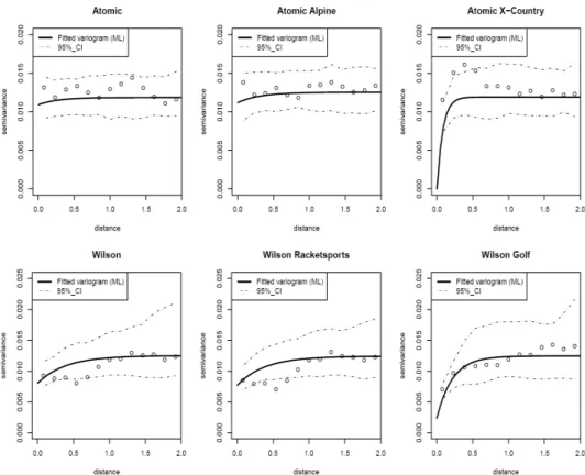
4.4.1 Semivariograms . . . 76

4.4.2 Model fitting results . . . 77

4.4.3 Prediction results . . . 80

4.5 Conclusions . . . 83

4.6 References . . . 84

4.7 Notes. . . 86

Part II: Non-linear causal inference

87

5 Causal discovery for heteroscedastic financial series 89

5.1 Introduction . . . 89

5.2 Causal discovery for heteroscedastic model . . . 91

5.2.1 First step: BAMLSS . . . 91

5.2.2 Second step: Bivariate CAM . . . 93

5.3 Simulation study . . . 94

5.4 Stock market indices . . . 101

5.4.1 Pairwise exploration . . . 101

5.4.2 Extension to multivariate case . . . 101

5.5 Conclusion . . . 104

5.6 Appendix . . . 105

Chapter 1

Introduction

In this thesis, I investigate two specific issues in data science, namely demand forecasting and causality inference. Let’s start by defining data science as an interdisciplinary field combining statistics and computer science, aiming to un-derstand and analyze actual phenomena through large databases. According to

Van der Aalst[2016], data science includes data extraction, preparation, explo-ration, transformation, data storage and retrieval, computing infrastructures, various types of mining and learning, presentation of explanations and predic-tions. Data science aims at providing meaningful information based on large amounts of complex data for decision-making purposes. Nowadays, data sci-ence is omnipresent in everyone’s everyday life. Applications of data scisci-ence are numerous. For example, receiving personalized advertisements related to our past online researches, the fact that YouTube shows all our favorite videos on our home screen, or healthcare parameters control through connected watches etc.

Moreover, in recent years, data science has become an essential component of many industries and fields.

• In biomedicine the application of data science on biomedical informa-tion such as human genome, provides an opportunity for personalized medicine programs in order to improve patient care through modern se-quencing technology allowing high-resolution genetic sese-quencing at tremen-dous scale [Costa,2014].

• In social science, professionals have now access to terabytes of data de-scribing almost instantly human behavior and interactions between in-dividuals, this allows them to study and try to understand contours of society through data science methodologies. For instance, Moussaïd et al. [2011] study pedestrian flows and crowd disasters. They suggest that, guided by visual information such as the distance of obstructions in individual lines of sight, pedestrians adapt their walking speeds and directions. Their model aims to predict individual trajectories and col-lective patterns of motion.

• To enter a market with specific characteristics, marketers have to segment the potential customers and understand their needs. For this purpose, data science is used to develop predictive and descriptive methods such

customer relationship management, for example customer behavior anal-yses in order to maximize expected customer value [Provost and Fawcett,

2013].

• Financial institutions were among the early users of data science. Data science is applied in numerous domains such as portfolio management, investment risk analysis, prediction of bankruptcy, etc. The use of data science helps the banks better understand customer needs and anticipate their response to new products and services [Dick, 2008].

Numerous other fields are impacted by data science. Our interest in data sci-ence is motivated by a desire to improve demand forecasting accuracy impact-ing supply chain performance on one hand, and to infer the causal relationship in the case of non-linearity and heteroscedasticity on the other hand, dividing this thesis in two parts.

Part 1: Demand forecasting

Supply chain management (SCM) plays an essential role in corporate efficiency. It consists of designing, planning, monitoring and optimizing supply chain activities, from supplying raw materials to delivering final products, in order to create net value and synchronize supply with demand. One way of achieving the goal of SCM is to minimize total costs with respect to frictions of different chain partners, for example considering the inventory level, the sale department will tend to opt for higher inventory levels in order to fulfill demands whereas the warehouse division will prefer lower inventories so as to reduce storage costs [Ayers, 2006; Sadeghi et al., 2016]. For the purpose of matching supply with demand, demand forecasting is a fundamental component of supply chain process. Historical operational and sales data are utilized to estimate the expected forecast of customer demand that are used for almost all supply chain related decisions such as:

• Optimization of inventory levels: the most accurate demand forecast allows an optimized management through right decisions concerning the whole process going from desired raw material to finished goods and their inventory level [Singh and Kumar,2011].

• Customer service/satisfaction level: proper forecast of customer demand helps to adapt the offering to a wide variety of customers. Indeed, un-derstanding the customer’s situation and need contributes to superior demand chain efficiency and high customer satisfaction [Heikkilä,2002]. Demand forecasting has been widely studied in both qualitative and quanti-tative reasoning approaches. Hofmann and Rutschmann [2018] showed that demand forecasting is a complicated task that could benefit from additional relevant data and processes and they examine how big data analytics improve the accuracy of demand forecasts. They found that the integration of different data sources in demand forecasting process is feasible but requires data scien-tists and appropriate technology investments. Hence the first part of this thesis consists studying how to enhance demand forecasting accuracy using pertinent data (e. g. operational transaction data, weather data, socio-economic data, etc.). Each article explores a new statistical approach on the supply chain optimization through demand forecasting accuracy.

Article 1:

Uncertainty has been proved to negatively affect supply chain performance [Dahistrom et al., 1996; Morris and Carter, 2005]. The starting point of the improvement of supply chain performance is to understand the customer’s demands in order to optimize the asset utilization, to eliminate the excess inventories costs and to reduce lead time. For this purpose, several studies focus on the impacts of extreme weather [Tierney, 1997; Blackhurst et al.,

2011]. The effects of weather on productivity has been more investigated than its effects on supply chain performance, especially in agricultural and construction industries [Thomas et al., 1999]. Since weather plays a role in the operational activities, the first article consists of studying how everyday weather fluctuations impact supply chain performance in different business of sport goods.

We analyze several business units with different operational strategies through real transctional business longitudinal data matched with daily location-based weather conditions (temperature, quantity of snow/rain, length of sunshine per day). We found that when the temperature increases the mean order volume significantly decreases for small customers in resorts ordering seasonal products in winter. In other words, weather at customer locations has a significant effect on order volumes and this effect differs according to the type of product, the location and the size of the customer; and non-urban locations or resorts seem more vulnerable than urban areas to weather variability. We also study ways in which weather fluctuations affect supply chain performance, that is, the delivery delay in days. We found that when the temperature increases, the delay in days also significantly decreases.

We were also interested in analyzing how weather fluctuations affect the de-pendence between order volume and delays. We found that order volume and delay are more dependent during winter than during summer.

The results of this article can be used to estimate and explain the weather effect in supply chain performance. Understanding this relationship is valu-able both for improving sales forecast accuracy and for improving operational performance.

Article 2:

Demand forecasts play a crucial role for supply chain management especially in case of seasonal products because of the conflict opposing retailers to manu-facturers concerning the order time. Indeed, due to the demand uncertainty of seasonal products, retailers tend to place their orders as late as possible in or-der to gather more information and reduce demand forecasting error, whereas manufacturers having limited productions capacity wish to have orders as soon as possible [Chen and Xu,2001]. According toChen and Yano[2010], weather is an important determinant of demand for the seasonal products. In the sec-ond article we aim to explain how weather csec-onditions and fluctuations affect the accuracy of demand forecasting for seasonal products, namely winter sport goods which are ordered and manufactured over 8 months before to be sold to customers, meaning a long lag between ordering and delivery. We analyze real transaction business data of alpine ski products of different brands matched

We found that weather conditions have a significant impact on demand fore-casting accuracy. The incremental improvement gained is the reduction in percentage errors up to 45%. The contribution of this article is the opera-tionalization of a ‘great winter’ and the demonstration of the fact that weather in one winter affects sales in the next winter. These results can be used to jus-tify and motivate the integration of the impact of variability in weather in the decision making process in order to better anticipate demand volumes and reduce costs due to excess inventory or stock shortages.

Article 3:

Seasonal products are common in many industries and can involve a large number of factors such as the influence of seasonal weather changes or socio-economic features. Since the weather characteristics such as temperature or precipitation, and socio-economics features are spatially dependent [Ashraf et al., 1997; Anselin, 1999], we assume that close customers are more likely to similar demand according to weather and socio-economic features and cus-tomers far apart from each other are more likely to have less similar demand. Numerous studies of seasonal products are based on time series statistical tech-nics [Adhikari and Agrawal, 2012; Gan et al., 2014] and less on geostatistics. Geostatistics have been applied to model the spatial dependence in various fields such as mining industry, soil science, agriculture etc.

Assuming that customers in a neighborhood may imitate each other leading to spatial dependence, we aim in the third article to improve demand forecasting accuracy by using the concept of spatial dependence and interpolation, and incorporating the effects of socio-economic aspects and weather conditions in the spatial dependence structure. We focus on studying the demand fluctu-ation of seasonal (winter sport goods) and unseasonal leisure goods (indoor sports and golf equipment). We analyse real demand data to find first how it varies geographically according to socio-economic aspects and weather condi-tions; and second how the additional information, i.e external to the supply chain, affects demand forecasting accuracy.

As main results we show that weather conditions impact the spatial correlation of the demand of seasonal products, but they do not have a significant impact for unseasonal products. We found that socio-economic features impact spatial correlation of both seasonal and unseasonal demand. The accuracy of demand forecasting is improved by the incorporation of weather conditions and socio-economic features in the forecasting process, the reduction of the forecasting error is up to 48%.

These results can be used in the decision making process, for example for plan-ning future demand in order optimize inventories and orders, or for deciding the location of a new retail shop.

Part 2: Causality inference

It is well known to anyone who has basic notions of statistics that "correla-tion does not mean causa"correla-tion". The most famous example is the link between country’s chocolate consumption and Nobel Prize victories [Messerli, 2012]. This article provides a graph showing a strong correlation between chocolate

capita as well. Since this correlation does not imply causation, we have three possibilities: Either chocolate influences Nobel price or the opposite, or both chocolate consumption and Nobel price are influenced by a common under-lying mechanism such as the country’s economic features and the investment capacity in research. Therefore, the best way to go from correlation to causal-ity is, identifying causal relationships from controlled randomized experiments [Rubin,1974], but these experiments are in many cases too costly or unethical and even infeasible.

Inferring causality from observational data is one of the fundamental subjects in empirical science. The alternative developed tools to controlled randomized experiments, are based on inferring causal relationships from observational data using conditional independence [Rubin, 1974; Pearl, 2009; Spirtes and Zhang, 2016]. In the bivariate case when observing only two variables (X

and Y), causality inference consists of identifying the direct causation "X → Y" or "X ← Y" with the assumption that there is no latent confounding variable causing both X and Y. In the additive context, this problem has been studied by imposing certain model specifications or restrictions. For linear causal models (Y = bX +ε), if at most one of X and ε is gaussian, the causal direction is identifiable, due to the independent component analysis (ICA) theory [Hyvärinen et al.,2004]. The linear non-Gaussian causal model, known as LinGAM [Shimizu et al.,2006] also relies on ICA with the additional assumption that disturbance variables have gaussian distributions of non-zero variances. Even though linear causal models with additive noise are often used because they are well understood and there are well-known methods, nevertheless in reality many causal relationships are more or less nonlinear. Nonlinearities in the data-generating process provide more information on the underlying causal system since these models allow more aspects of the true data generating mechanisms to be identified (Y = f(X) +ε) [Hoyer et al.,

2009]. The post-nonlinear causal model (Y =g(f(X) +ε)) provided by [Zhang and Hyvärinen, 2009] aims to distinguish the cause from effect by analyzing the nonlinear effect of the cause, the inner noise effect, and the measurement distortion effect in the observed variables. According to the literature review, most of the papers analyze additive models with either linearity, nonlinearity or gaussian noise, the case of a nonlinear and non-gaussian causal multiplicative noise model (Y =f(X) +g(X)ε) has been less explored.

In finance, causality is mostly studied conditioned on time. For example, the linear and nonlinear intertemporal cross correlation [Atchison et al.,1987] aims to infer causality according to time. This method relies on the fact that asset prices change in a time-lag manner and not simultaneously. In other words, price-adjustment delay factors along with nonsynchronous trading cause the autocorrelations present in daily asset returns.

The most explored is the widely used Granger causality [Granger and Morgen-stern,1963]. Under Granger causality, the cause happens prior to its effect. It aims to determine whether one time series is useful in forecasting another. A time series X is said to Granger-cause Y if it can be tested that lagged val-ues of X provide statistically signicant information about future values of Y.

Granger[1981] provides a cointegrated form causality based on the fact that, in finance, assets can move in an integrated manner, meaning that they evolve

nonlinear integrated dependencies function. More precisely two time series are considered as cointegrated when their combination is stationary. For the linear case if asset X is negatively cointegrated with asset Y, this means that if the price of assetX increases at timet−1, then the price of asset Y shall decrease at time t. Besides the up cited methods, numerous time series models aim to infer causal dependencies nevertheless they are all conditioned on time, hence one cannot observe assets and infer the causality simultaneously.

Article 4:

Inferring causality between financial assets is a common and fundamental sub-ject in nance. We have seen that most of the existing methods are conditioned on time. In this paper, we aim to infer the intrinsic causal mechanism between two financial heteroscedastic time series. Unlike the Granger causality which infers only at the mean level, we investigate causal relations not only in mean but from the perspective of location, scale and shape parameters of the under-lying distribution. We propose a new two-steps method Causal Heteroscedastic Model (CHM) that is not conditioned on time and can handle any response distribution since it infers the inherent causality through all the parameters of the underlying distribution. We focus on the bivariate multiplicative noise model Y =f(X) +g(X)ε. The two-steps CHM consists of applying a causal additive model (CAM) on the BAMLSS (bayesian additive model for location, scale and shape) fitted values of the estimated parameters. We have tested our method on both simulated and real financial indices log-returns data. We found that CHM reaches the accuracy of 0.97 on average. On financial data we fitted both bivariate and the multivariate CHM, we find an intrinsic causal effect of the shares on the index they compose. The multivariate analysis pro-vides directed acyclic graphs (DAG) revealing the causal structure between shares in normal and extreme case. This new method is a real contribution to causality research since it can deal with any response distribution and it is applicable to many other domains in future research, such as genomics etc.

Conclusion

In this thesis, I have explored and analyzed two specific subjects in data science, which are Demand forecasting and Causality inference. With proper demand forecasting, supply chain and business performance can be consid-erably improved, resulting in numerous benefits, such lead time reduction, storage costs reduction and more important customer satisfaction. This thesis has provided several studies improving demand forecasting accuracy by reduc-ing the forecastreduc-ing error in several contexts dealreduc-ing with seasonality, through the integration of external data such as weather or socio-economic data, using complex statistical models.

The causal method provided in this thesis allows the inference of inherent causal mechanism between assets unconditioned on time. The developed Causal Heteroscedastic Model is applied to financial index data highlighting ground-truth causal evidence and opens wide the door to numerous other applications in finance or any other domain dealing with heteroscedasticity.

Part I: Demand forecasting using

weather

Chapter 2

Weather and supply chain

performance in sport goods

distribution

Weather and supply

chain performance in sport

goods distribution

Patrik Appelqvist

Amer Sports Corporation, Helsinki, Finland, and

Flora Babongo, Valérie Chavez-Demoulin,

Ari-Pekka Hameri and Tapio Niemi

Faculty of Business and Economics, University of Lausanne,

Lausanne, Switzerland

Abstract

Purpose–The purpose of this paper is to study how variations in weather affect demand and supply chain performance in sport goods. The study includes several brands differing in supply chain structure, product variety and seasonality.

Design/methodology/approach –Longitudinal data on supply chain transactions and customer

weather conditions are analysed. The underlying hypothesis is that changes in weather affect demand, which in turn impacts supply chain performance.

Findings–In general, an increase in temperature in winter and spring decreases order volumes in resorts, while for larger customers in urban locations order volumes increase. Further, an increase in volumes of non-seasonal products reduces delays in deliveries, but for seasonal products the effect is opposite. In all, weather affects demand, lower volumes do not generally improve supply chain performance, but larger volumes can make it worse. The analysis shows that the dependence structure between demand and delay is time varying and is affected by weather conditions.

Research limitations/implications–The study concerns one country and leisure goods, which can limit its generalizability.

Practical/implications – Well-managed supply chains should prepare for demand fluctuations

caused by weather changes. Weekly weather forecasts could be used when planning operations for product families to improve supply chain performance.

Originality/value–The study focuses on supply chain vulnerability in normal weather conditions while most of the existing research studies major events or catastrophes. The results open new opportunities for supply chain managers to reduce weather dependence and improve profitability.

KeywordsWeather, Demand variation, Seasonal products,

Supply chain management and performance

Paper typeResearch paper

1. Introduction

Due to their multi-level structures, many events can disturb supply chain performance in several ways. Unplanned events may affect value and product processes, assets and infrastructures, inter-organizational networks through man-made and environmental causes (Peck, 2005). The more complex the supply chain is the more vulnerable it is to risks emerging from the supply and demand side, as well as catastrophic risks like natural hazards (Wagner and Bode, 2006). Major events or catastrophes make the news headlines and have significant consequences on societies, businesses and individuals. Along with the most memorable events, there have been severe but less extent incidents, such as European heat waves in 2003 and 2006, which were devastating and destroyed crops and affected businesses and their value chains. These and

International Journal of Retail & Distribution Management Vol. 44 No. 2, 2016 pp. 178-202

© Emerald Group Publishing Limited 0959-0552 DOI 10.1108/IJRDM-08-2015-0113 Received 12 August 2015 Revised 19 August 2015 21 October 2015 Accepted 7 December 2015

The current issue and full text archive of this journal is available on Emerald Insight at: www.emeraldinsight.com/0959-0552.htm

178

IJRDM

44,2

similar events surely had a negative impact on supply chains, yet for some reason they seem to be within normality in their occurrence, and companies and people are expected to cope with them.

However, everyday weather-related fluctuations also affect supply chain performance in different business and supply chain contexts. Although these weather fluctuations, and even severe local weather conditions, occur frequently, most existing research focuses on rare major weather events or catastrophes and the vulnerability of supply chain operations. To fill this gap in the existing research, we focus in this paper on normal daily fluctuations in weather conditions by studying the following research question:

RQ1. Do everyday changes in weather conditions have an effect on demand, and in turn on supply chain performance measured by delivery punctuality?

Our research is based on analysing real transactional business data that covers over a decade of operations and supply chain-related transactions for seven different business units. These individual units are owned by a publicly listed brand holding company delivering well-known sporting equipment and goods to customers worldwide. The business units differ in operational strategy, product variety, country of origin, demand variability (seasonality) and predictability. The business data will be matched with daily location-based weather conditions (temperature, quantity of snow/rain, length of sunshine per day).

Our research methods include using a generalized linear model (GLM) to explain changes in demand and the delay in delivery based on local weather conditions, and then analysing the dependence between these using a generalized additive model and a copula approach. Our results show that, in addition to the order volume, customer locations and weather conditions affect supply chain performance. Further, this relationship is not constant but it depends on the season and weather conditions when resort locations are considered. The results can be used in many ways for improving supply chain performance. An example of this would be to remove bias caused by weather variables to measure the true supply chain performance of the company, to prepare the supply chain for higher volumes or variations in demand based on weather forecasts, or even to re-engineer supply chains which are less weather dependent.

Our study deals with weather events that are considered as normal in variation and which do not make the major headlines. We do not study floods, earthquakes and tsunamis, but the variation in performance and non-resilience in supply chains faced with normal fluctuations in weather conditions. We study orders made by business customers during business days, for example, retailers or ski rental companies, and delivery efficiency to them. Thus, end customer behaviour is beyond our scope. Since these normal changes in weather conditions do not have a direct effect on movement of goods, efficiency in factories, or logistics, we focus on weather at the customer’s geographical locations.

We start by reviewing the literature on supply chain performance and vulnerability with a special focus on weather and its influence on performance. We seek to find gaps in the body-of-knowledge to form our detailed research hypotheses. The applied statistical methodology is then explained along with the description of the data used for the analysis. This is followed by a detailed analysis section after which the results are discussed from theoretical and practical points of view. We will also assess the internal and external validity of the work done. Finally, conclusions are drawn and avenues for future research are presented.

179

Weather and

supply chain

performance

2. Literature review on weather affecting operations and supply chain management

Disruptions and process variance lead to poor supply chain performance. There is ample literature including case studies, models and surveys on the costly consequences of dysfunctional supply chains. In their seminal study, Hendricks and Singhal (2003) show that companies reporting problems in sourcing and delivery, product quality, etc., are associated with an abnormal decrease in shareholder value by 10.28 per cent. These problems refer to a vast multitude of incidents embedded in modern supply chains and researchers have classified and modelled these causes for poor supply chain performance in many ways.

For more than a decade research on supply chain risk, vulnerability and security has flourished and become a discipline of its own. Motivation for this research has increased ever since the 9/11 terrorist attacks (Sheffi, 2001), various epidemics (Giunipero and Eltantawy, 2004) and natural hazards and other drastic disruptions in the business environment (Kleindorfer and Saad, 2005; Sheffi, 2005; Sheffi and Rice, 2005). In their thorough analysis on supply chain disruptions, vulnerability and mitigation, Stecke and Kumar (2009) show that incidents negatively affecting supply chain performance have increased over time. These incidents include natural catastrophes, terrorist attacks, social unrest, major accidents and other mishaps that affect the increasingly complex and physically longer supply chains with increased numbers of exposure points. With regards to weather they hint that advanced companies do take forecasts into account when planning material flows. In their thorough study on supply resiliency, which results in a comprehensive framework, Blackhurst et al. (2011) treat weather as an extreme disturbance. Similarly, most of the literature on supply chain vulnerability concerns mainly major events and weather is only referred to in an extreme context.

Christopher and Lee (2004) emphasize the role of information sharing when mitigating supply chain risk while at the same time building confidence among the partners in the chain. In a similar vein, in their survey of supply chain professionals, Craigheadet al.(2007) find that early warning systems and rapid distribution of information to various players in the supply chain are vital to prevent and prepare for potentially hazardous events. These warning systems should also include information on changes in weather, that is, should a ship be a day late or a truck a few hours off schedule. Delays in sharing information also imply delays in corrective measures, as demonstrated in the famous mobile phone industry case in which a storm triggered a fire at a critical component supplier’s warehouse paralyzing the industry for several weeks (Norrman and Jansson, 2004; Latour, 2001). Although with no direct reference to weather, Manuj et al. (2014) indicate that postponement and reasonable speculation in supply chains may fall short of mitigating operational supply chain risk. They emphasize that it is vital to understand the total cost and system implications related to the importance of a stable and reliable supply base, the nature of demand variability, and the cost of finished goods inventory are reviewed first. The impact of weather on productivity has been studied more widely than its impact on supply chain performance, especially in construction and agricultural industries. Thomaset al. (1999) quantified the effect of weather on a construction site and found significant losses in productivity because of snow (41 per cent) and cold temperatures (32 per cent). Seasonal industries have also examined the impact of weather. In their study on the construction industry, Rojas and Aramvareekul (2003) conclude surprisingly that external factors, notably weather and temperature, which are often cited as a major cause for reduced productivity, are considered to be one of the least relevant productivity drivers.

180

IJRDM

44,2

As Van der Vorstet al.(1998) show, even if average consumer demand is known there are always variations due to weather changes and changing consumer preference. The traditional way to respond to weather-induced fluctuations is by keeping inventory. From perishable goods to services, keeping inventory and reactive capacity are important as they are the main means to maintaining service level (Chopra and Lariviere, 2005). Further, Van der Vorst and Beulens (2002) study supply chain uncertainties through three case studies that were also vulnerable to weather. They indicate that weather plays a variation generating role both in up- and-downstream supply chains, especially when agricultural and perishable products are concerned. In general, in food chains weather causes variation both in demand and supply and this should be taken into account There are some indications that seasonal production, products and services tend to be more vulnerable to changes in weather (Costantinoet al., 2013), which partially explains the use of production smoothing and reactive capacity.

Clark and Hammond (1997) study the retail industry and the impact of electronic commerce to speed up reordering processes. They point out that efficient service also requires taking into account regional weather conditions (e.g. higher inventories are needed in Maine than in California due to snow and hurricanes) and that this is possible due to shorter replenishment cycles and information sharing. Following similar reasoning, Sheffi and Rice (2005) mention a company-specific weather service at a global parcel carrier incorporating weather fluctuations in their daily operational planning, which enables them to rapidly reroute to maintain the service level.

Aviv (2001) presents and formalizes the concept of collaborative forecasting as a means of improving supply chain performance. Even though the model is abstract, in a well concerted situation with continuously updated situational information, it could also take into account changes in weather. Chaharsooghi and Heydari (2010) study ways in which mean and variance in lead time affect supply chain performance. As lead time at each echelon of the supply chain plays a major role in the overall performance of the whole chain, they analyse whether the focus should be on the reduction of the mean or the variance. They show that focus on variance has a greater impact on supply chain and inventory performance, yet to tame the bullwhip effect focusing on reducing the lead time mean is more important. Ways to manage weather-induced variation are limited. However, as indicated earlier, being prepared via inventory and reactive capacity is one way to handle it. One could also prepare for fluctuations caused by weather through planning that extends beyond organizational boundaries.

Various financial instruments like rebates and derivatives also provide companies with a means of protecting themselves against disruptions and problems caused by weather. The development of weather derivatives represents one of the recent trends towards the convergence of insurance and finance (Brockett et al., 2005). Chen and Yano (2010) show that the use of price fluctuations and hedging against bad weather, by using weather derivatives, could improve supply chain performance in weather intensive seasonal products. These tools aim to share supply chain risk along the downstream players of the supply chain. These and other statistical methods related to risk management have been applied to the supply chain context. These instruments are relatively new and mainly concern certain industries and markets. They are beyond the scope of our research, although there could be further uses for them in highly seasonal and weather dependent businesses.

There are many studies on the effect of the weather on consumer behaviour and demand. Bahng and Kincade (2012) study women’s business wear and show strong evidence that fluctuations in temperature can impact sales of seasonal garments.

181

Weather and

supply chain

performance

During sales periods when drastic temperature changes occur, more seasonal garments are sold. However, the temperature changes from day to day or week to week do not affect the number of garments sold for the whole season. They also show that fluctuations depend on the fabric and design.

Murray et al. (2010) study how weather affects consumer spending and the underlying psychological phenomenon. They especially focus on the sunlight effect. The authors recognize, based on the literature, three general categories: first, bad weather reduces people’s willingness to go shopping; second, the weather has a direct effect on some products, such as ice-cream; and finally, the weather can affects the consumers’ “internal states”. The study contained sales and weather data for a period of six years. They find that an increase in sunlight tends to increase consumer spending but this effect also depends on temperature: at lower temperatures the effect is positive but negative when temperatures are high.

In agriculture, Behe et al. (2012) study the influence of weather on the sale of different plants (vegetables, flowers, etc.). Their conclusion is that the weather has an impact but it is weaker than that of the weekday, region, or month. Other examples of the weather effect on consumer decision making is a study by Busse et al. (2015) on how the weather conditions affect car sales. They find that the weather on the purchase day has a significant impact on the sales of convertibles and 4×4 vehicles. Bertrand et al. (2015) study how unseasonal weather affects apparel sales and how companies can deal with this risk. They use a linear regression model to estimate the impact of temperature differences on sales volumes in the apparel retail business.

There are also several studies on effects of external events such as weather on stock market behaviour. Levy and Galili (2008) study how cloudiness affects people’s mood and their stock market transactions. They find differences among investor groups relative to how the weather affects their decision making. They conclude that, in cloudy weather, men, lower income and young people buy more stocks than other groups. In the same spirit, Lu and Chou (2012) study weather effects and stock index returns. Their conclusion is that weather can affect trading activities but not returns. Finally, an example of the influence of weather on the electricity market can be found in Huurman et al.(2012) who study the weather premium in the electricity market. They show that using the next day weather forecast clearly improves electricity price predictions.

As the literature review above illustrates, research into the effects of weather on supply chain performance is limited to overall classification of issues making supply chains vulnerable and ways in which major disruptions impact global supply chains. Weather plays a role in the operational planning of transportation, retail and seasonal businesses. However, the impact of fluctuations in temperature and sunshine duration on supply chain performance has not been systematically studied. Few case studies show that advanced companies can adjust and react to changes in weather, and can actually gain a competitive advantage from it (Ishikawa and Nejo, 1998). Common knowledge and some of the research shows that weather is blamed for poor performance, although this has not really been proven and the evidence is based on limited case-based surveys and anecdotal evidence.

3. Research hypotheses, data and methodology

Based on the existing literature, academics have paid limited research interest to weather and its impact on supply chain performance. On the one hand strong evidence supports the fact that weather affects demand and consumer shopping behaviour (Murray et al., 2010; Parsons, 2001), and on the other hand, fluctuations in demand

182

IJRDM

44,2

affect supply chain performance (e.g. Beamon, 1999). But the overall chain of reasoning from fluctuations in weather affecting demand variation leading to variance in supply chain performance has been less studied. Although this effect is observed in some cases, it is not possible to establish such a general straight hypothesis. Therefore, this research aims to fill the gap in the current supply chain body-of-knowledge by studying ways in which weather affects demand in different market locations and different customer and product segments.

3.1 Building up detailed research hypotheses

By using longitudinal data covering about a decade of operations in several business units totalling over 300,000 deliveries of different sporting goods and matching these deliveries with daily weather data in different locations in Switzerland, we study the link between changes in weather, demand and supply chain punctuality. Depending on the product type, for example, summer or winter items, the change in temperature may have a different impact on demand, thus we analyse the direction of change in temperature. On the other hand, we assume that the greater the increase in order volumes measured in monetary value, the more the demand fluctuates, which in turn increases supply chain load and therefore a decrease in supply chain performance and punctuality.

The weather data holds daily information on the temperature differences to the long-term average, precipitation and sunshine duration relative to daily maximums. This data are location specific enabling us to divide our customers according to their geographical location into urban vs resort areas. We assume that resorts are more prone to demand fluctuations induced by changes in temperature, sunshine and snow fall. In urban areas meteorological changes may have less impact on demand than in resorts where people are more exposed to practicing activities related to the products studied. Our first hypothesis reads:

H1. Non-urban places, that is, resorts are significantly exposed to demand fluctuations induced by weather.

We then study seasonality. Some of the business units are seasonal (e.g. skiing equipment for winter sports), while others are by nature non-seasonal (e.g. sports instruments, certain apparel with relatively constant demand patterns). Seasonal here means that manufacturing, sales and actual deliveries take indistinct phases and overlap very little. These business units face the planning problematic depicted by the newsvendor model according to which one has to order goods in stock before facing actual and uncertain demand. For non-seasonal businesses the fluctuations in demand are smaller, and demand variations easier to anticipate, thus seasonal businesses are more prone to weather-induced disruptions in demand. Therefore we assume that seasonal businesses are more vulnerable to fluctuations in weather, and that they face more supply chain delays. Therefore the second hypothesis is:

H2. Supply chain performance (punctuality in terms of delay) for seasonal business is more vulnerable to supply chain load (order volume in local currency) than it is for non-seasonal business. Furthermore seasonal businesses and their supply chains react differently to fluctuations of weather than non-seasonal businesses. The customers, meaning the retailers, speciality and sport shops, etc., vary hugely in sales volume and the amount of stock keeping units they hold. By sales rank we differentiate between small and large customers. We assume larger customers order more frequently and have more choice to offer and thus they hold larger buffers to

183

Weather and

supply chain

performance

mitigate demand fluctuations. Therefore they also face better supply chain performance than smaller customers. On the other hand, as larger customers order larger volumes, changes in weather may increase their ordering volumes relatively more than the same weather changes for smaller customers. Thus larger customers may face more supply chain delays. On the other hand, smaller customers may be more reactive to changes in weather thus doing more rush orders and therefore they may be faced with more frequent supply chain delays. As the literature and our reasoning leads to differing views on how weather affects supply chain performance large and small customers, we write the third hypothesis in the following general form:

H3. Weather has a different impact on large and small customers’ ordering behaviour, which in turn, affects their supply chain delay.

The three previous hypotheses state separately the effects of different variables on supply chain performance and on order volume. We then study the effects of these independent variables on the dependence between delay and order volume. If there is a relationship between high demand and delay, this association should be less significant in summer but it increases in resorts when the weather conditions deteriorate. This leads to our last hypothesis:

H4. The dependence between demand volume and supply chain performance is seasonal and is affected by weather in resort areas.

The statistical analysis shows that these hypotheses are not independent and therefore may not be studied separately. In Section 4, we precisely formulate our findings, looking at the significant interactions between the different variables and for different seasons of the year. Altogether the hypotheses make it possible to devise statistically justified sentences on the multidimensional relationships related to customer size, geographical location, seasonality, and weather fluctuations. The original motivation for the study stems from the supply chain management of the underlying case company, and their willingness to drill in to the very impact of weather on their supply chain performance. They have hands on knowledge and experience spanning over several years indicating that weather has an impact on their performance, yet they do not have a unanimous view on it and opinions tend to vary over the years along with financial results.

3.2 The case company and data

The case company, established in 1950, has a long history of commodity products. In the end of the 1980s a decision was made to transform the company entirely into a sporting goods company. The first sporting goods brand was acquired in 1989 followed by another four acquisitions over the next 15 years. At the time of the study, the company owned seven global business units providing customers with sports equipment for a range of summer and winter sports, indoor and outdoor sports, sports instruments as well as fitness equipment. We chose five brands for this study:

(1) Salomon (seasonal): alpine skiing, cross-country skiing, snowboarding and trail running;

(2) Atomic (seasonal): alpine skiing;

(3) Wilson (non-seasonal): tennis, baseball, American football, golf, basketball, softball, badminton and squash;

184

IJRDM

44,2

(4) Suunto (non-seasonal): sports precision instruments; and (5) Precor (non-seasonal): premium-quality fitness equipment.

At the centre of our study are three constructs, namely, weather, supply chain load and operational performance. Weather is a construct formed by temperature and daily sunshine. Supply chain load is measured by order volumes in local currency and the operational performance of the supply chain is measured as a delay in days between actual and planned delivery date. The business contexts are urban vs resort customer residence areas and the delivery is destined for seasonal vs non-seasonal product families and small vs large customers. The data consist of 307,300 in-season orders in Switzerland and the corresponding delivery delays observed from March 2003 to December 2012. The in-season orders as opposed to pre-seasonal orders are driven by the situational constraints related to weather, overall demand and business expectations, and they are supposed to be delivered right away.

Products are manufactured or sourced based on sales plans for the following six to 12 months. Sales plans are based on historical sales, commercial insight and on open orders. Especially for seasonal products open pre-season orders provide a valuable source of information for making accurate sales forecasts. Products are distributed via regional distribution centres located in Austria, France and Germany. These distribution centres serve customers in all European countries, and are in some cases also replenished by regional distribution centres in Asia and the Americas. Manufacturing and sourcing volumes are defined using multi-level MRP, considering manufacturing capacity in its own and in supplier factories. The target of this production planning is to maintain a balance between high delivery precision and low inventory levels.

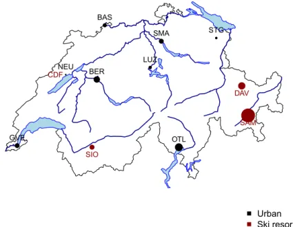
Switzerland is a mid-size country in terms of company sales. Products are typically delivered directly to shops. At the time of the data sample, own retail and e-commerce were still very small scale. There were no country-specific distribution facilities in Switzerland. The country was divided into twelve different areas classified as urban and holiday resorts. The urban areas were located around the cities of Basel, Bern, Geneva, Locarno, Lucern, Neuchâtel, Zurich, St-Gallen, while the studied holiday resorts are La Chaux-de-Fonds, Davos, Samedan (St. Moritz) and Sion. The data were collected from the enterprise resource management system that is used to manage each brand (for the data structure, see Table I). The data harmonization and integration process took place in phases as new brands were acquired.

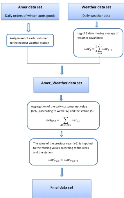
The weather data were retrieved from the national weather database containing weather statistics on all weather stations in Switzerland. The data were matched with the chosen urban and resort areas mentioned above. The weather data holds continuous daily values on the key variables and a relevant geographical location related to main sales areas. Three of the resorts are in the mountain area, two of them being well-known ski resorts. The rest of the resorts are in main cities in Switzerland. We retrieved the temperature difference from the long-term average, as explained in the next section, and daily sunshine duration relative to possible daily maximum. The database for the analysis was built by merging the supply chain data and weather data based on the date and location. Each data item has the following form: customer, order ID, order time, order line value, delivery time, delay, weather station, customer size, postal code, product group, product ID, weather variables. For the weather variables we use moving average over the past five days.

185

Weather and

supply chain

performance

Figure 1 shows the histogram for the logarithm of order line values. We use a GLM to explain the logarithm of the mean order line value, which we use to indicate the order volume. We use the following explanatory variables (covariates):

• _{Place: customer location either an urban city or a ski resort; and}

• _{Period/season of the year: we define three main periods of a year that we call}

winter (from November to February), spring (from March to June) and summer (from July to October).

There are statistical reasons for having split the year in three main seasons: first the four formal seasons lead to too few data per season in the analysis and second, the decomposition which actually integrates formal“autumn”in Summer and Winter shows most significant effects among all possible yearly break downs by blocks of three months. We also checked seasonality in demand by adding the “day-of-year”covariate using a non-parametric form allowed by

Order line Sales document Product hierarchy

Sales document number Sales document number Product hierarchy

Item Sales doc type Description

Material number Sales organization Brand

Quantity Created by Material group

Value Sold-to party Material group

Plant Ship-to party Description

Shipping point Material Customer

Created on Material number Customer number

Requested delivery date Material description Zip code

Realistic GI date Product hierarchy Country

Actual GI date Material group

Confirmed delivery date Material type Customer pick-up date Retail intro date Ready pack date

Table I.

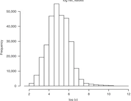
The structure of the supply chain transaction data 50,000 F requency 40,000 30,000 20,000 10,000 0 2 4 6 log (y) log net_values 8 10 12 Figure 1. Histogram of the logarithm of order volumes measured in monetary value

186

IJRDM

44,2

generalized additive models. The effect exists but it is negligible under this non-parametric form. Thus, we decided to use a factor “season”instead.

• _{Product type: we differentiate between seasonal (Atomic, Salomon) and non-seasonal}

(Suunto, Precor, Wilson) products.

• _{Customer type: small or large (determined by individual size in sales volume from}

the case company to customer): small customers are those below the median of the empirical individual size and large customers are above it. The orders among these groups are distributed as follows: small customers in urban areas 39 and 11 per cent in ski resorts; large customers in urban areas 37 per cent and in ski resorts 13 per cent.

• _{Weather variables: we use moving average over the past five days of}

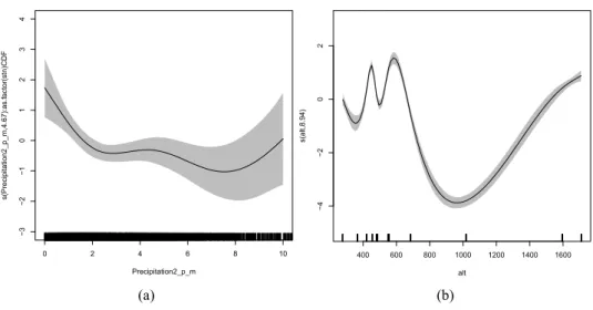
“temperature”(T). This is the temperature at 2 meters above ground which is a deviation from the daily maximum in relation to the “norm 6190” (norm 1961-1990). This variable is continuous and its histograms for the three periods are shown in Figure 2. The distributions are skewed, especially in spring, highlighting a warmer deviation from the norm (1961-1990). For the sake of interpretation, and in order to make it a factor, for each period of the year, we differentiate two levels of temperature: the low level called LowTemp for which the temperatures are below the median of all the temperatures observed for the related period of time, and HighTemp which represents the temperatures below the median. Similarly, we also use sunshine duration (high and low) and precipitation (high and low) as covariates but it turns out that these two are not significant to explain the demand.

3.3 Explaining weather effect for demand

We use a GLM to explain the mean value of an order lineµby the set of covariates listed above. The model readsµ¼ e(Xβ), whereXis the vector of covariates andβthe vector of coefficients. The general purpose of the GLM model is to quantify the relationship between several predictor variables, their possible interactions and a dependent variable. The model explains the significance of predictor variables and it can also be used for forecasting values of the dependent variable. In our current case, the covariates areplace, period,product type,customer type and weather variablesand the dependent variable is the mean value of an order line which we use to indicate theorder volume.

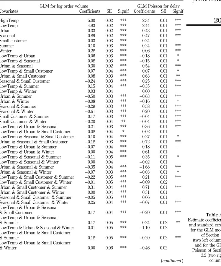
To find the most suitable model, several models including different covariates (X) are fitted and compared using the likelihood ratio statistic which is a standard test for nested models. We use the 5 per cent confidence level to retain significant covariates. Based on this procedure, the significant covariates are: place(urban vs resort), period (winter, spring or summer), product type (seasonal vs non-seasonal), customer type (small vs large) andtemperature variable (LowTemp vs HighTemp). The interactions between the covariates are also significant. The goodness of fit of the model is assessed by standard diagnostics on residuals. The residuals are the error terms, that is, the differences between the fitted values (obtained from the model) and the observed values (the data).The resulting estimate coefficients are listed in Table AI in the three left columns. The table provides the coefficient estimates (β), their standard errors for all significant covariates and their interactions and the level of significance given by the stars. TheR2of the model is about 21 per cent. The coefficients with the largest values correspond to the most significant factors in the model. The covariates, or their

187

Weather and

supply chain

performance

Winter Spr ing Summer 12,000 8,000 6,000 Frequency Frequency Frequency 4,000 2,000 0 8,000 4,000 2,000 0 10,000 8,000 6,000 6,000 4,000 2,000 0 –10 –5 0 5 10 –10 –5 0 5 10 –5 0 5 10 Figure 2. Histograms of the temperature variable for winter (left), spring (middle) and summer (right)

188

IJRDM

44,2

interactions that do not appear, are set to 0. An example of using the table to calculate the mean value of order lines is the following: for a small customer in a resort ordering a seasonal product in winter during a low temperature period (Tomedian), the estimate mean of order lines is (in CHF):

eð4:93þ0:890:03þ0:28þ0:08þ0:070:24þ0:030:610:200:10:01þ0:25þ0:07Þ ¼223:63: Whereas the same characteristics (covariate levels) but for high temperature (TWmedian) gives an estimate mean order line value of CHF 208.51. The decrease in mean order line value when the temperature increases from LowTemp to HighTemp corresponds to one of the global trends discovered in our detailed analysis. If needed, one can provide confidence intervals for the estimators using the standard errors. One way to check these fitted values from the model is to compare them with the actual mean values observed in the data set. For the low temperature period, the actual mean was 222.19 and for the high temperature period 207.89. The predicted values from the model are therefore very close to the actual values.

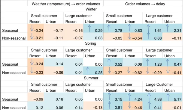
The resulting GLM model can be used to predict the effect of weather variables on order volumes (with an uncertainty level) but it does not directly show the actual effects. Therefore, based on the significant coefficients of the model, we constructed tables (Table II, Section 4) using the actual data with rows and columns representing the levels of the different covariates. These tables clearly show the observed impact of the weather (temperature) on order volume.

Small customer Large customer Small customer Large customer

Resort Urban Resort Urban Resort Urban Resort Urban

Seasonal –0.24 –0.17 –0.16 0.29 0.78 0.83 1.61 2.31

Non-seasonal –0.21 –0.11 –0.07 0.03 –0.05 –0.54 0.88 –0.11

Small customer Large customer Small customer Large customer

Resort Urban Resort Urban Resort Urban Resort Urban

Seasonal –0.24 0.14 0.04 0.00 0.52 0.06 1.28 0.47

Non-seasonal –0.23 –0.06 0.04 0.25 –0.27 –0.62 –0.29 –0.41

Small customer Large customer Small customer Large Customer

Resort Urban Resort Urban Resort Urban Resort Urban

Seasonal –0.09 0.18 0.05 0.00 3.15 4.24 4.38 5.17

Non-seasonal 0.12 0.06 0.14 –0.13 0.81 –0.46 0.41 –0.01

Spring

Summer Winter

Weather (temperature) → order volumes Order volumes → delay

Notes: The numbers show the relative proportional difference for the given season. For instance, –24 per cent is the relative decrease in percent of order volumes for a small customer in a resort for a seasonal product in winter due to an increase of temperature. Only significant changes are shown by an arrow at the level of 5 per cent significance. Red means a decrease and blue an increase: the more intense the colour, the more significant the effect. It is possible to provide confidence intervals for the true proportions but they are not provided here to keep the paper focused

Table II. Increase in temperature effect on order volume (left blocks) and increase in order volume on delay (right blocks) during winter (top blocks), spring (middle blocks) and summer (lower blocks) seasons at different combinations of customer size, location and product type

189

Weather and

supply chain

performance