c
EXPLOITING SPARSITY FOR MACHINE LEARNING IN BIG DATA
BY
RONGDA ZHU
DISSERTATION
Submitted in partial fulfillment of the requirements
for the degree of Doctor of Philosophy in Computer Science
in the Graduate College of the
University of Illinois at Urbana-Champaign, 2017
Urbana, Illinois
Doctoral Committee:
Professor Chengxiang Zhai, Chair
Professor Jiawei Han
Assistant Professor Jian Peng
Doctor Yu Deng, IBM Research
Abstract
The rapid development of modern information technology has significantly facilitated the generation, collec-tion, transmission and storage of all kinds of data. With the so-called “big data” generated in an unprece-dented rate, we are facing significant challenges in learning knowledge from it. Traditional machine learning algorithms often suffer from the unmatched volume and complexity of such big data, however, sparsity has been recently studied to tackle this challenge. With reasonable assumptions and effective utilization of sparsity, we can learn models that are simpler, more efficient and robust to noise.
The goal of this dissertation is studying and exploiting sparsity to design learning algorithms to effectively and efficiently solve various challenging and significant real-world machine learning tasks. I will integrate and introduce my work from three different perspectives: sample complexity, computational complexity, and noise reduction. Intuitively, these three aspects correspond to models that require less data to learn, are more computationally efficient, and still perform well when the data is noisy. Specifically, this thesis is integrated from the three aspects as follows:
First, I focus on the sample complexity of machine learning algorithms for an important machine learning task, compressed sensing. I propose a novel algorithm based on nonconvex sparsity-inducing penalty, which is the first work that utilizes such penalty. I also prove that our algorithm improves the best previous sample complexity significantly by extensive theoretical derivation and numerical experiments.
Second, from the perspective of computational complexity, I study the expectation-maximization (EM) algorithms in high dimensional scenarios. In contrast to the conventional regime, the maximization step (M-step) in high dimensional scenario can be very computationally expensive or even not well defined. To address this challenge, I propose an efficient algorithm based on novel semi-stochastic gradient descent with variance reduction, which naturally incorporates the sparsity in model parameters, greatly economizes the computational cost at each iteration and enjoys faster convergence rates simultaneously. We believe the proposed unique semi-stochastic variance-reduced gradient is of general interest of nonconvex optimization of bivariate structure.
To overcome the noise in the text data which hampers the detection of real events, I design an efficient algorithm based on sparsity-inducing fused lasso framework. Experiment results on various datasets show that our algorithm effectively smooths out noises and captures the real event, outperforming several state-of-the-art methods consistently in noisy setting.
To sum up, this thesis focuses on the critical issues of machine learning in big data from the perspective of sparsity in the data and model. Our proposed methods clearly show that utilizing sparsity is of great importance for various significant machine learning tasks.
Acknowledgements
First of all, I would like to express my most sincere gratitude to my advisor Professor Chengxiang Zhai for his support and care during my PhD study. Professor Zhai is both a great researcher and a helpful advisor. He provides me with effective and insightful guidance when I run into difficulties, and also grants me great independence and freedom on my research at the same time. His passion for research always moves me deeply and encourages me to explore the unknown. I am very blessed to have him as my advisor. Without his help and guidance, this thesis would not have been possible.
I want to thank Professor Jian Peng, for his help and guidance in my PhD research work on sparsity in event detection. His knowledge, acumen and dedication inspire me and I have really learned a great deal from him. I am also grateful to the other two great researchers in my PhD committee, Professor Jiawei Han and Doctor Yu Deng, for their constructive comments and advices for this thesis. Doctor Deng was my intern manager at IBM research. She gave me great support and contributed a lot to my PhD research.
I would also like to thank Professor Quanquan Gu from University of Virginia. He led me into machine learning research systematically and sparked my genuine interest in sparsity. He also helped me a lot with the technical details of my research work.
I owe special thanks to my all friends and labmates in the group including Aston Zhang, Yinan Zhang, Hongwei Wang, Hongning Wang, Mingjie Qian, Yanen Li, Jingjing Wang, Xiaolong Wang, Jialu Liu, Sheng Wang, Shan Jiang, Xueqing Liu, Sean Massung, Chase Geigle, Jason Cho, Ismini Lourentzou, Yang Liu, Yiren Wang and every DAIS group member. Thanks for your help and encouragement!
Finally, I would like to thank my families for their wholehearted love and care, which support me to overcome all the difficulties. This thesis is dedicated to them.
Table of Contents
Chapter 1 Introduction and Motivation . . . 1
1.1 Lower Sample Complexity for Robust One-bit Compressed Sensing . . . 2
1.2 Accelerated Stochastic Gradient Expectation-Maximization Algorithm . . . 3
1.3 Noise Reduction in Event Detection . . . 4
Chapter 2 Related Work . . . 5
2.1 One-bit Compressed Sensing . . . 5
2.2 High Dimensional EM Algorithm . . . 6
2.3 Event Detection with Noise Reduction . . . 7
2.4 Sparsity . . . 9
Chapter 3 Lower Sample Complexity for Robust One-bit Compressed Sensing . . . 10
3.1 Background . . . 10
3.2 Nonconvex Penalty Functions . . . 11
3.3 One-bit Compressed Sensing with Nonconvex Penalty . . . 12
3.4 Theoretical Results . . . 15
3.4.1 Oracle Property of Our Estimator . . . 16
3.4.2 Sample Complexity of Our Estimator for Strong Signals . . . 22
3.4.3 Sample Complexity for General Signals . . . 25
3.5 Experiments . . . 30
3.5.1 Approximate Vector Recovery for General Signals . . . 30
3.5.2 Approximate Vector Recovery for Strong Signals . . . 31
3.5.3 Support Recovery . . . 32
3.5.4 Oracle Property . . . 33
3.6 Summary . . . 34
3.7 Proofs and Technical Details . . . 35
3.7.1 Proof of Lemma 3.3.1 . . . 35
3.7.2 Proof of Lemma 3.3.2 . . . 37
3.7.3 Derivation of Algorithm 1 . . . 37
3.7.4 Derivation of Algorithm 2 . . . 38
3.7.5 Auxiliary Technical Lemmas . . . 41
Chapter 4 A Stochastic Gradient EM Algorithm with Improved Computational Com-plexity . . . 42
4.1 Introduction and Background . . . 42
4.2 Stochastic Variance Reduced Gradient . . . 44
4.3 Semi-stochastic Gradient EM with Variance Reduction . . . 45
4.3.1 Latent Variable Models . . . 45
4.3.2 Semi-stochastic Variance Reduced Gradient EM . . . 46
4.4 Main Theory . . . 47
4.4.1 Technical Conditions . . . 48
4.4.3 Implications on Specific Models . . . 57
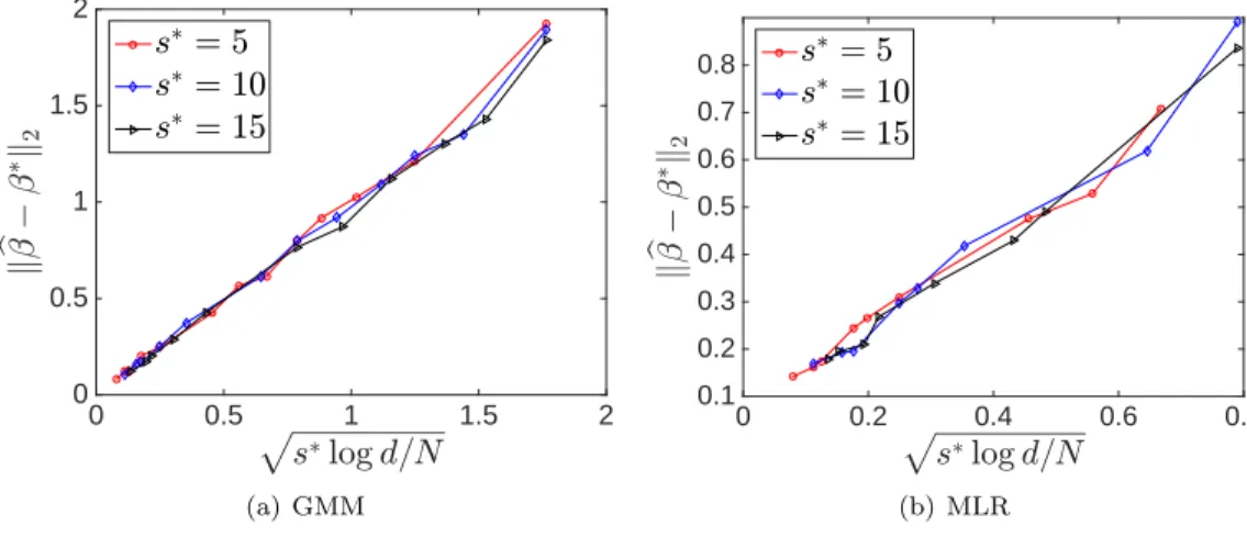
4.5 Experiment Results . . . 63
4.5.1 Experimental Setup . . . 64
4.5.2 Gaussian Mixture Model . . . 64
4.5.3 Mixture of Linear Regression . . . 64
4.5.4 Statistical Rate of Convergence . . . 65
4.6 Summary . . . 66
4.7 Proofs and Technical Details . . . 68
4.7.1 First-order Stability . . . 69
4.7.2 Statistical Error . . . 78
Chapter 5 Event Detection with Noise Reduction . . . 84
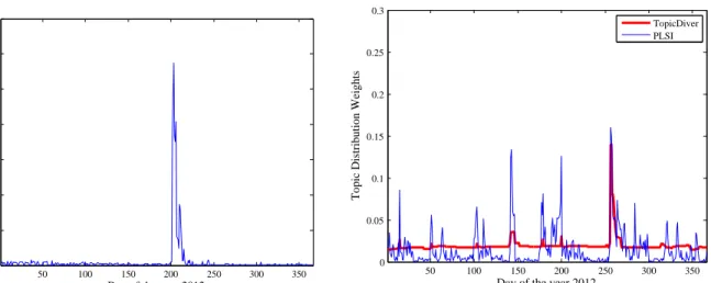
5.1 Topic Distribution . . . 84
5.2 Problem Formulation . . . 86
5.3 Proposed Method . . . 87
5.3.1 Probabilistic Latent Semantic Indexing (PLSI) . . . 87
5.3.2 TopicDiver: A Longitudinal Regularized Mixture Model . . . 88
5.4 Optimization Algorithm . . . 89 5.5 Experiments . . . 91 5.5.1 Datasets . . . 92 5.5.2 Evaluation Metrics . . . 92 5.5.3 Experiment Design . . . 94 5.5.4 Experimental Results . . . 95 5.5.5 Parameter Setting . . . 96 5.6 Summary . . . 97
Chapter 6 Conclusion and Future Work . . . 98
Chapter 1
Introduction and Motivation
Datasets in this era grow at a rapid pace across various fields of engineering and science. For example, the prosperity of online social media has led to overwhelming amount of text data; wireless sensor networks are gathering physical and environmental data such as temperature, sound and voltage; biomedical data are accumulating on computers and servers and facilitating the research of genomics and proteomics. Due to the enormous scales and complexity of these datasets, how we can efficiently learn simple and useful knowledge from them emerges as a critical challenge in this so-called “big data” era.
While such unprecedented massive amounts of data provide us with huge opportunities, conventional machine learning algorithms also show their limitations. Generally speaking, the framework of a learning algorithm is that it takes a certain training dataset as input and learns a desired objective through a designed computation process. Correspondingly, there are three important aspects for evaluation of a learning algorithm, in terms of the quantity and quality of the training dataset, and the complexity of the computation process:
• Sample Complexity. Sample complexity measures the number of samples a machine learning al-gorithm needs, so that the function returned by the alal-gorithm is within an arbitrary small error of the best possible function, with probability arbitrary close to 1. In other words, a better learning algorithm in terms of sample complexity should need fewer examples to achieve a certain error bound with high probabilities.
• Noise Reduction. The input data can always be disturbed by irregular fluctuations and perturbances which is often referred to as noises. Noise reduction steps such as Gaussian smoothing and wavelet smoothing are often adopted to overcome such undesirable noises and facilitate the learning process. A robust learning algorithm should be able to address the noise challenge and still achieve desirable performance in the noisy settings.
• Computational Complexity. Computational complexity concerns the computational resources a learning algorithm needs to learn the desired target from the input dataset. In big data scenario, the
computational complexity has particularly been a rising challenge due to the scale and complexity of the data. Traditional methods may face prohibitive cost.
In order to better meet our needs in high dimensional and big data scenario, it’s crucial that we pro-pose learning algorithms improved from all three aspects above, i.e., algorithms requiring less examples for training, more robust to noise and more computationally efficient for learning.
To tackle such significant challenges in big data scenario, sparsity has been widely studied and used as a workhorse. Despite the ubiquitous high dimensional and complex data, many real-world signals and processes are concurrently sparse. For example, in speech recognition and image processing, the signals are often sparse in frequency domain or under some other appropriate basis; in biomedical research, only a few genes out of a huge number are of interest to a certain hereditary feature; in online social media, there are vast amount of short text snippets with sparsity in vocabulary. In some scenarios, we also want our learned models to be sparse, for lower computational cost and better interpretability. By exploring intrinsic sparsity of the data or applying reasonable sparsity assumptions, this thesis aims at learning compact, efficient and robust models that best fit the scale and dimensionality of this big data era.
This thesis attempts to exploit the sparsity in the data and model, and address the aforementioned three challenges. Specifically, we target at three important tasks in machine learning and text mining, i.e., one-bit compressed sensing, high dimensional expectation-maximization (EM) and event detection, and improve previous best results in the aspects of sample complexity, computational complexity and noise reduction by developing novel algorithms incorporating sparsity.
1.1
Lower Sample Complexity for Robust One-bit Compressed
Sensing
The first component of this thesis is an efficient and robust algorithm for one-bit compressed sensing which improves the sample complexity significantly. Compressed sensing is the technique to recover a sparse signal using a few linear measurements. As we know, Nyquist rate is usually required for measurements to exactly recover the unknown signal [1]. However, when the signal is sparse, i.e., only a few entries are nonzero, we can restore the unknown signal with much fewer measurements by sophisticated measurement matrices and recovery algorithms. While conventional compressed sensing uses real-valued measurements, one-bit
compressed sensing utilizes only one-bit, i.e., the sign of the measurements. Therefore, one-bit compressed sensing is often more robust to noise and non-linearity.
sensing, which is used to denote the number of measurements needed for an algorithm to obtain an estimator of the signal with error bounded by constant. For example, the sample complexity of [2], a convex estimator by linear programming, is O(slog2d/5). Such sample complexity means that when the signal dimension isdand at most sentries are nonzero, the algorithm needs O(slog2d/5) one-bit measurements to find an estimator with the estimation error bounded by. For the one-bit compressed sensing problem, it is crucial that we improve the sample complexity of algorithms to accommodate the scale and complexity of the data in high dimensional and big data scenarios. My proposed algorithm based on nonconvex penalty functions improves the sample complexity of the recovery of strong signals significantly from previous best results O(slogd/2) toO(s/2), which is especially important for the high dimensional regime.
1.2
Accelerated Stochastic Gradient Expectation-Maximization
Algorithm
The second contribution of this thesis focuses on the computational complexity. We propose an accelerated EM algorithm based on stochastic gradient. EM algorithm is widely used as a popular algorithm for the estimation of latent variable models. However, in high dimensional cases, the maximization step (M-step) can be time consuming or even not well defined. Therefore, the more general gradient EM algorithms, where the M-step is based on gradient ascent, have been attracting increasing research attention. However, these algorithms can still be computationally prohibitive in big data scenarios, since they need to compute the full gradient in each iteration.
To address this great challenge of computational complexity, we propose a novel algorithm based on a unique semi-stochastic gradient, where we only need to compute the gradient over a mini-batch each time. Our work is also the first method that brings variance reduction into the EM algorithm to overcome the intrinsic variance of stochastic gradient. The specially designed semi-stochastic structure and variance re-duction distinguish our work from all existing methods. Our algorithm is proved to reduce the computational and concurrently outperform the state-of-the-art methods in terms of estimation error. Specifically, we show that with an appropriate initialization, our estimator achieves a linear convergence with the statistical rate of convergence matching the best previous result up to a logarithmic factor.
1.3
Noise Reduction in Event Detection
The third part of this thesis is noise reduction in event detection from text data. With the overwhelming text information, event detection has emerged as an important task that can significantly helps us understand the large-scale text data, such as scientific literature and social media. However, this detection process is often hampered by the heavy noise in the data. Therefore, noise reduction is always of great necessity for more accurate event detection in both retrospective and online settings.
I propose a novel event detection based on the undiscovered temporal divergence of topic distributions to tackle this challenge. I find that enforcing sparsity in this divergence greatly helps with the noise issue. Sparsity-inducing longitudinal regularization is applied to such divergence to effectively combat the noise and capture the real events. Our proposed algorithm can be smoothly adapted to both retrospective and online settings, and is also scalable to work on social media like Twitter.
Organization: The rest of this thesis is organized as follows. In Chapter 2, I discuss the representative related work. I present my work on one-bit compressed sensing in Chapter 3, high dimensional EM in Chapter 4 and event detection from text data in Chapter 5 . Finally, Chapter 6 concludes the thesis and discusses potential future work.
Notation: Let A = [Aij] ∈ Rd×d be a matrix and v = (v1, . . . , vd)> ∈ Rd be a vector. We define the
`q-norm (q≥1) of v as kvkq= P d j=1|vj|q
1/q
. Specifically, kvk0 denotes the number of nonzero entries of v, kvk2 =
q Pd
j=1v 2
j and kvk∞ = maxj|vj|. For q ≥ 1, we define kAkq as the operator norm of A.
Specifically, kAk2 is the spectral norm. We let kAk∞,∞ = maxi,j|Aij|. For an integer d > 1, we define
[d] ={1, . . . , d}. For an index setI ∈ [d] and vector v ∈Rd, we use v
I ∈ Rd to denote the vector where
[vI]j=vj ifj∈ I, and [vI]j = 0 otherwise. We use supp(v) to denote the index set of its nonzero entries,
and supp(v, s) to denote the index set of top s largest |vj|’s. C, C0, C1, C2, . . . are used to denote some
absolute constants. The values of these constants may be different from case to case. LetkXkψq (q≥1) be
the Orlicz norm of random variable X. λmax(A) and λmin(A) are used to denote the largest and smallest eigenvalues of matrixA. We useB(r;β) to denote the ball centered atβ with radiusr.
Chapter 2
Related Work
In this chapter, we discuss the related work in details. Specifically, we will review the existing literature by the machine learning tasks we focus on separately: one-bit compressed sensing, high dimensional EM algorithm and event detection.
2.1
One-bit Compressed Sensing
One-bit compressed sensing was first introduced in [3] where the authors minimized the `1 norm of a unit vector which is consistent with the measurements, and further shown effective recovering sparse signals from nonlinearly distorted measurements [4]. Suppose x∗ is the unknown signal vector, and {ui}ni=1 is a set of measurement vectors. The sign of real-valued measurement is observed as follows:
yi= sign(hui,x∗i), i= 1,2, . . . , n
whereyiis the binary one-bit measurement we use.
In general, there are two major tasks in one-bit compressed sensing: (1) approximate signal vector recov-ery [5, 6, 7], which aims at finding an estimatorxbwith an estimation errorkbx−x∗k2 small enough; and (2) support recovery, which finds the support, i.e., positions of the nonzero entries [5, 8, 9].
For the first task, approximate signal vector recovery, it is worth noting that since only the sign of the real-valued measurements are used, we cannot recover the magnitude of the signal, i.e., we always assume that the signalx∗ is a unit vector with kx∗k2 = 1, which further makes this problem nonconvex. A convex formulation is proposed in [2], where`1 norm is put on the measurement vectors instead of signal vectors. The sample complexity of this work isO(slog2d/5), whereis the guaranteed estimation error bound. [10] also proposed a popular convex approach by maximizing the dot product of the one-bit measurements and the real-valued measurements. Their sample complexity isO(slogd/4).
The best previous results in terms of sample complexity for approximate vector recovery is achieved in [7]. The authors proposed an efficient algorithm with close-form solution based on `1 regularization. Their
sample complexity isO(slogd/2).
For the second task, support recovery, we have the current best sample complexity of O(slogd) in [9]. However, their result depends on specially designed measurement matrices based on the signals, thus not universal. A universal method for support recovery is proposed in [5], which is based on two combinatorial structures: union free families of sets and expanders. For their method, all signals can be recovered using a single measurement matrix. The sample complexity isO(s2logd).
Gaussian measurements are used in the majority of the cases for its generality, and recently one-bit compressed sensing is also extended to non-Gaussian measurements [11]. The authors use sub-Gaussian measurements to recover both exactly and approximately sparse signals that are not extremely sparse. Other extensions have also been studied. For example, in [12] the sparse signals to be recovered can be with unknown and time-variant sparsity levels and the measurements are noisy. [13] studied one-bit compressed sensing on piece-wise smoothing signals.
Most of the previous studies only focus on one of the two major tasks. In contrast, my proposed algo-rithm [14] is proved to improve the best previous sample complexity significantly and achieve exact support recovery at the same time. At the core of my algorithm is nonconvex sparsity-inducing penalty function, which has been studied and utilized in various fields of statistics [15, 16, 17, 18]. My work is the first ever study to introduce such penalty functions into the problem of one-bit compressed sensing.
2.2
High Dimensional EM Algorithm
EM algorithm and its variants [19, 20] are widely used for the estimation of latent variable models and studied for a long time [21, 22, 23, 24]. There has been a long history of convergence analysis for EM algorithms [20, 25], however, only until recent research efforts [26, 27, 28] do we have rigorous understanding on the statistical convergence guarantees of EM algorithms.
The first study of definite statistical rate of convergence was introduced in [26], where the authors showed that with a suitable initialization, their algorithm can always converge to a reasonable local optima at a linear rate. Nonetheless, their work is only for low dimensional regime. The conventional EM algorithm as well as its gradient variants were extended to the high dimensional setting in [27], where the number of parameters of the latent variable is comparable to or even larger than the number of data points. According to their study, EM algorithms in the high dimensional regime must be carefully regularized by sparsity-type assumptions. Specifically, they applied a truncation step (T-step) after the M-step at each iteration. Another relevant study was introduced in [28], where the authors used a regularized estimator in M-step. It
is worth noting that all of the methods mentioned above are deterministic requiring the computation of full gradient at each iteration.
In order to avoid the prohibitive computational complexity in large-scale optimization [29, 30], stochastic gradient methods are always a popular workaround. For such methods, we only need to compute a partial gradient based on a stochastic mini-batch of data. However, the inherent variance is another challenge which hampers the convergence rate of stochastic methods [31, 32]. Accordingly, variance reduction techniques are studied to overcome this challenge. One of the most popular methods is the stochastic variance-reduced gradient (SVRG) [33], which has been widely utilized for a lot of optimization problems [34, 35, 36], and even for nonconvex problems [37, 38] for variance reduction.
Nonetheless, all the previous studies only tackle the univariate scenario, i.e, the optimization depends on only one variable. In EM algorithm, the structure is bivariate, and whether variance reduction can be applied to such structure is still remained to be seen. To the best of our knowledge, our work [39] is the first algorithm that incorporates variance reduction into EM algorithms in the high dimensional regime.
It is worth noting that reasonable initialization is a necessary condition for the convergence and statistical guarantees of high dimensional EM algorithms. Without a proper initialization, the estimator can be far away from the true model parameter and statistical properties of the objective function may not apply. Therefore, it is possible the estimation error accumulates instead of converges along the iterations. For different latent variable models such as Gaussian mixture model and mixture or linear regression, there are various spectral methods [40, 41] that helps with the initialization.
2.3
Event Detection with Noise Reduction
In a collection of documents, events are significant and novel stories. The discovery of such significant stories that have not been aforementioned, known as event detection, is often of great importance in understanding the data. For example, event detection on scientific literature can greatly help new researchers understand how the research interests evolve over time [42]; event detection on Twitter has been a popular approach to discover the bursty or trending topics and public interests [43], and even faster earthquake detection has been proposed using such methods [44].
Existing studies on event detection can be generally classified into two categories: • document-pivot methods.
Document-pivot methods focus on clustering the documents and analyze these clusters of documents to find features for events. A representative method is used in the UMASS system [45] exploitingterm frequency– inverse document frequency (TF-IDF) weight vectors to represent the document features, and identifies a new document as an event if it is different enough from all existing clusters. Otherwise, it is assigned to the closest cluster and the cluster center is updated. This method has achieved best performances in several topic detection and tracking (TDT) competitions. To make the UMASS system efficient enough for working on social media scale like Twitter, [46] improved the scalability by locality-sensitive hashing (LSH).
Feature-pivot methods aims at detecting the statistical patterns of the corpus and get event features from these patterns, which can be term frequency, term cooccurrences and distributions.
For example, in [47], the frequency of each term is modeled by a binomial distribution. The bursty features are detected as a set of words when the parameters of these distributions change. They use a set of cooccuring bursty features to feature a detected events. This idea is further extended to an event hierarchy construction in [48], where the documents are clustered based on their bursty features into a hierarchical event structure. In [49], Discrete Fourier Transform (DFT) is applied to extract the bursty features from term frequency. Since frequency-domain techniques are involved, this method naturally distinguishes periodic and aperiodic events well.
With the increasing popularity of user-generated data such as citizen journalism and social media, the “noise” in data is also emerging as a significant challenge. For example, meaningless “babbles” [46] are generated at a very high rate on Twitter. A straightfoward solution was proposed in [50], where the authors simply used the hash tag #breakingnews to pick the valuable news posts out of the noises. The wavelet signals generated from term frequency was first used in [51] to filter out the noises. Specifically, the authors determine all the signals with the auto-correlation lower than a threshold as trivial. They then cluster the terms based on cross-correlation of different wavelet signals. To group the similar Tweets which might be of short length, the weight of proper nouns is boosted in TF-IDF weighting. The temporal and geographical features of social media such as Twitter are also important for event detection. For example, [52] proposed an event detection framework based on time and location-based topics.
As we have introduced, feature-pivot methods [43, 47, 48, 51] study the distribution of terms and detect events by clustering these terms. By nature, these methods are closely related to topic models which aim to extract hidden topics from text data and also characterize these topics by word clusters. Static topic models such as probabilistic latent semantic analysis (PLSI) [53] and latent Dirichlet allocation (LDA) [54] have gained great success, and time is also incorporated [55, 56, 57] to discover evolving topics in text corpus. Specifically, an online variant of LDA with applications to event detection was proposed in [57]. The authors
learn the model in an incremental fashion, where the model from last iteration passes its parameters to the next iteration as priors. Then word distributions of models from two consecutive iterations are compared to see if there is enough difference indicating an event. This model is further extended to a dynamic vocabulary in [58].
Despite the increasing research attention on topic model-based methods on event detection, most of them detect the events by exploiting the divergence of word distributions of topics. The topic distributions of documents featuring the coverage of topics in the corpus, have not received research attention. Our work is the first study that looks into topic distributions for the problem of event detection.
2.4
Sparsity
Sparsity is utilized in a wide variety of machine learning problems [18, 59, 60], which helps us learn more compact and interpretable models with lower sample and computational complexity. As we have mentioned, sparsity is ubiquitous especially in high dimensional scenarios. Therefore, it is often reasonable to apply sparsity-inducing regularizers to enforce sparse structure in high-dimensional data or models. The most commonly used techniques include`-0 regularization [61, 62, 63] and`-1 regularization [64, 65, 66].
In this thesis, we incorporate sparsity to our machine learning algorithms from different perspectives. We look into different sparse-inducing regularization functions, and apply them to the output of our models. In our work, we focus sparsity in both the original data and resulting model.
More specifically, in our work on one-bit compressed sensing, sparsity is in the signal we want to recover; in our work on stochastic gradient EM algorithm, we want to enhance sparsity in the model parameters we learn; in the event detection problem, we also enforce sparsity in the parameter we learn to better encode the nature of real events. We can see that sparsity can really be exploited flexibly to match our needs in different machine learning tasks.
Chapter 3
Lower Sample Complexity for Robust
One-bit Compressed Sensing
In this chapter, I will present my work on one-bit compressed sensing [14]. I propose an efficient algorithm with close-form solution, achieving a significantly improved sample complexity for vector recovery and exact support recovery simultaneously.
3.1
Background
We first briefly describe the general framework of one-bit compressed sensing. We let x∗ is the unknown signal vector, andkx∗k0≤s. {ui}ni=1is a set of measurement vectors and the one-bit measurements are the signs of real-valued measurements observed as follows:
yi= sign(hui,x∗i), i= 1,2, . . . , n.
Our goal is to recoverx∗ from{(yi,ui)}ni=1. Note that in one-bit compressed sensing the norm of the signal does not affect the measurements, thus we let kx∗k2 = 1. We focus on the more realistic noisy setting,
whereyi can be influenced by irrational perturbances. As described in [10], we assumeyican be treated as
independently drawn from a distribution with the following expectation
E(yi|ui) =θ hui,x∗i, i= 1,2, . . . , n
whereθ(z) is the function modeling the expectation with value domain [−1,1]. We define
E[θ(g)g] =:γ >0, (3.1.1)
whereg∼N(0,1) is a standard Gaussian random variable, andγmeasures the correlation betweenyi and
hui,x∗i. When the noise is not significant, these two are well correlated, which means that γ will get a
higher value. Whenyi is equal to sign(hui,x∗i), there is no noise and γwill get the maximal value
p 2/π.
3.2
Nonconvex Penalty Functions
At the core of my framework is the nonconvex penalty functions. In this work, we also have these functions as decomposable Gλ,b(x) = d X i=1 gλ,b(xi),
whereGλ,b(x) is the decomposable function on the signal vector andgλ,b(xi) is the component function on
the entries. λandb are regularization parameters shaping the function.
There are a variety of nonconvex penalties that are decomposable. Representatives include the smoothly clipped absolute deviation (SCAD) penalty [15] and minimax concave penalty (MCP) [16]. Specifically, MCP is given by gλ,b(t) = λ|t| − t 2 2b, if|t| ≤bλ, bλ2 2 , if|t|> bλ, (3.2.1)
where b >0, λ > 0 are fixed regularization parameters. An important property ofgλ,b(t) is that it can be
written as the sum of a`1penalty part and a concave part hλ,b(t) :gλ,b(t) =λ|t|+hλ,b(t).
Our work does not depend on specific form of gλ,b(t), such as MCP or SCAD. Generally, our work only
depends on the following conditions ongλ,b(t) andhλ,b(t):
C1. g0
λ,b(t) = 0,for|t| ≥ν ≥0.
C2. h0λ,b(t) is monotone, and fort0> t, there is a constantζ−≥0 such that
−ζ−(t0−t)≤h0λ,b(t 0)−h0 λ,b(t). C3. hλ,b(0) =h0λ,b(0) = 0. C4. |h0 λ,b(t)| ≤λfor anyt.
The above conditions hold for a wide variety of nonconvex penalty functions. For example, it can be proved that MCP and SCAD are valid choices. Specifically,ν =bλ andζ− = 1/bfor MCP. I use MCP as
the nonconvex penalty function in my algorithm, andg,G andh,Hwill be used to denote the component and sum functions of MCP in (3.2.1) and its concave part for the rest of this thesis.
3.3
One-bit Compressed Sensing with Nonconvex Penalty
We start with the framework of passive algorithm for one-bit compressed sensing [7], which is given by
argmin
kxk2≤1
−1 nx
>Uy+τkxk1 (3.3.1)
whereU is the measurement matrix. Since the estimator should be reasonably consistent with the one-bit measurements, we need to maximize the dot product ofU>xandy, which is the first part in (3.3.1). The second part is a`1 regularizer to enforce sparsity of the estimator.
Accordingly, our estimatorbxis any local optimal solution to the following optimization problem
argmin kxk2≤1 − 1 n n X i=1 yihui,xi+Gλ,b(x) + τ 2kxk 2 2, (3.3.2)
where u1,u2, . . . ,un ∈ Rd are the rows of the known measurement matrixU ∈ Rn×d, and Gλ,b(·) is the
nonconvex penalty function. I use `2 regularizer here. I will later show why the penalty function and regularizer are necessary.
I also propose a novel algorithm to efficiently compute the estimator as the local minima in (3.3.2). The basic idea here is divide and conquer. We denotev=U>y/n∈Rd for simplicity.
To go over the details of the proposed algorithm, we start with the following lemma tackling the subproblem of the optimization in (3.3.2).
Lemma 3.3.1. The solution to the following optimization problem
b x= argmin x 1 2(x−y) 2+g λ,b(|x|) is given by • if b >1 b x= S(y, λ) 1−1/b, if|y| ≤bλ, y, if|y|> bλ, (3.3.3) • if b≤1 b x= 0, if|y| ≤√bλ, y, if|y|> √ bλ, (3.3.4)
whereS(y, λ) is the soft-thresholding operator [67] defined forλ≥0 by S(y, λ) = y−λ, ify > λ, 0, if|y| ≤λ, y+λ, ify <−λ. Proof. Forb >1, please see [68]. Forb≤1, please refer to Section 3.7.
A similar version of Lemma 3.3.1 withτ >0 can be derived easily.
Lemma 3.3.2. The solution to the following optimization problem
b x= argmin x 1 2(x−y) 2+g λ,b(|x|) + τ 2x 2 is given by • if b(1 +τ)>1 b x= S(y, λ) 1 +τ−1/b, if|y| ≤bλ(1 +τ), y 1 +τ, if|y|> bλ(1 +τ). (3.3.5) • if b(1 +τ)≤1 b x= 0, if|y| ≤pb(1 +τ)λ, y 1 +τ, if|y|> p b(1 +τ)λ. (3.3.6)
Proof. Please see Section 3.7.
From Lemma 3.3.3 and 3.3.4, we can see that the decomposed subproblems in (3.3.2) have close-form solutions.
Now we are in position to solve (3.3.2). For the sake of simplicity, we first consider the case whereτ= 0 to illustrate our method. Theτ >0 case can be solved similarly, as we will show later.
We consider the Lagrange functionf(µ) of (3.3.2) given by f(µ) = min x −x >v+G λ,b(x) +µ(kxk22−1) = min x 2µ 1 2kx− v 2µk 2 2+ Gλ,b(x) 2µ ! −kvk 2 2 4µ −µ = 2µ X i min xi 1 2 xi− vi 2µ 2 +gλ/(2µ),2µb(|xi|) ! −kvk 2 2 4µ −µ, (3.3.7)
where the last equation comes from the property of MCP. We useµ∗to denote the optimal solution to the dual problem.
According to Lemma 3.3.1, we divide the problem into two cases: (1) 2µb≤1 and (2) 2µb >1. For each subproblem in (3.3.7), we can just determine the value ofµby dividing the feasible region ofviinto intervals
where the optimal value of µ can be determined. The outlines of our algorithms for these two cases are outlined in Algorithm 1 and 2 respectively.
I will only briefly introduce the algorithms in two cases, and the derivation and technical details of Algorithm 1 and 2 can be found in Section 3.7.
• 2µb ≤ 1: In this case, the solution to (3.3.7) comes from (3.3.4). Therefore, we need to compare the value of |vi/2µ| and λ
p
b/2µaccording to Lemma 3.3.1, which is equivalent to comparingµ and v2
i/2bλ2, to decide the value of each term in the summation in (3.3.7). After sorting|vi|and dividing
the feasible region into intervals, we will compute f(µ) and find µ∗ within each interval, which has a close form solution as in Line 5 to 11 of Algorithm 1 to getf(µ). Finally, among the optimal solutions in each interval, we findµ∗1 that maximizesf(µ).
• 2µb >1: In this case, the solution to (3.3.7) comes from (3.3.3). We do similar sorting and dividing operation, yet within each interval, we need to solve a simple optimization as in Line 8, Algorithm 2. Then we will find the finalµ∗2 by comparing the values from each interval.
After finding the optimal values ofµfrom the above two cases, we compare the objective function values of outputs of Algorithm 1 and 2 to get the finalµ∗:
µ∗= argmax µ∈{µ∗ 1,µ ∗ 2} f(µ). (3.3.8)
The optimal primal solution is further given by
b x= argmin x 1 2kx− v 2µ∗k 2 2+ Gλ,b(x) 2µ∗ .
By Lemma 3.3.1, we would finally get our estimator as follows: • if 2µ∗b >1 b xi= S(vi, λ) 2µ∗−1/b, if|vi| ≤2µ ∗λb, vi 2µ∗, if|vi|>2µ ∗λb. • if 2µ∗b≤1 b xi= 0, if|vi| ≤ p 2µ∗bλ, vi 2µ∗, if|vi|> p 2µ∗bλ.
For the caseτ >0, we have a similar Lagrange functionf(µ0) withµ0=µ+τ /2. The optimization off(µ0) is in a similar manner.
Algorithm 1Find maximizer of f(µ) whenµ≤1/2b
1: Input: λ, b,v 2: Output: µ∗1 3: Initializef=f(1/2b), µ∗1 = 1/2b 4: v(1), v(2), ..., v(d) =Sort(|v1|,|v2|, ...,|vd|) 5: v(0)= 0, v(d+1)=∞ 6: l=Find(v(l)≤1/2b < v(l+1)) 7: fori:=0 ... ldo 8: if q Pn j=iv 2 (j)/2∈(v 2 (i)/2bλ 2, v2 (i+1)/2bλ 2]then 9: µ= q Pd j=iv 2 (j)/2 10: else 11: µ=v2(i+1)/2bλ2 12: end if 13: if f(µ)> f andµ <1/2bthen 14: f=f(µ), µ∗1=µ 15: end if 16: end for
3.4
Theoretical Results
We will prove that under a reasonable assumption on the elements of the true signal x∗, our estimator will have oracle property, i.e., identical to the oracle estimator, with high probability. This indicates exact support recovery. We will also show the advantage of our method in terms of sample complexity.
Algorithm 2Find maximizer of f(µ) whenµ >1/2b 1: Input: λ, b,v 2: Output: µ∗2 3: Initializef=f(1/2b), µ∗2 = 1/2b 4: v(1), v(2), ..., v(d) =Sort(|v1|,|v2|, ...,|vd|) 5: v(0)= 0, v(d+1)=∞ 6: l=Find(v(l)≤1/2b < v(l+1)) 7: fori:=l...ndo 8: S1=Pnj=i+1v(2j) 9: S2=Pij=l(|v(j)| −λ)2 10: J(µ) = S4µ1 +2(2µS−21/b) +µ 11: if µi= argminµJ(µ)∈(|v(i)|/2bλ,|v(i+1)|/2bλ]then 12: µ=µi 13: else 14: µ=|v(i+1)|/2bλ 15: end if 16: if f(µ)> fandµ >1/2bthen 17: f=f(µ), µ∗2=µ 18: end if 19: end for
3.4.1
Oracle Property of Our Estimator
We will start with presenting the oracle property of the proposed estimator in (3.3.2). The definition of the oracle estimatorbxO is given by
b xO= argmin supp(x)⊂S,kxk2≤1 LO(x), (3.4.1) where LO(x) =−1/nP n
i=1yihui,xi. We can see that for the oracle estimator, the support information is
known as prior knowledge. The oracle property for an estimator is indicating this estimator is identical to the oracle estimator.
It is worth noting that support information is critical to the problem of one-bit compressed sensing. With the support information, the recovery problem will be much easier. Therefore, oracle property is often a strong criteria for estimators.
For the rest of this chapter, we use the following notations
Hλ,b(x) = d X i=1 hλ,b(xi) =Gλ,b(x)−λkxk1, L(x) =LO(x) + τ 2kxk 2 2=− 1 ny >Ux+τ 2kxk 2 2, e Lλ(x) =L(x) +Hλ,b(x) =− 1 ny >Ux+τ 2kxk 2 2+Hλ,b(x). (3.4.2)
Lemma 3.4.1. If τ ≤ kvSk2 where v = −1/nP n
i=1yiui and S is the support of x∗. The following
optimization problem b x= argmin supp(x)⊂S,kxk2≤1 −1 n n X i=1 yihui,xi+ τ 2kxk 2 2, (3.4.3)
has the same solution as the oracle estimator in (3.4.1).
Proof of Lemma 3.4.1. We will first give the following lemma which features the close-form solution for the oracle estimator.
Lemma 3.4.2. The following optimization problem
b x= argmin supp(x)⊂S,kxk2≤1 −1 n n X i=1 yihui,xi, (3.4.4)
has closed form solution, i.e.,
b xj= vj/kvSk2, ifj ∈S, 0, otherwise. wherev= 1/nPn i=1yiui= 1/n·U>y.
Proof. To solve the optimization problem in (3.4.4), it is sufficient to
argmin
kzk2≤1
−hvS,zi. (3.4.5)
The Lagrange function of (3.4.5) is
L(z, α) =−vS>z+α(kzk22−1).
Taking the gradient ofL(z, α) with respect tozand setting it to zero, we obtain
−vS+ 2αz= 0. (3.4.6)
Therefore, we havez= 1/(2α)vS. Substituting it back into (3.4.5), we obtain the dual problem as follows
argmin α − 1 4αkvSk 2 2−α. (3.4.7)
The optimal solution to the dual problem (3.4.7) is α∗ =kvSk2/2. Substitutingα∗ back into (3.4.6), and
solving forz, we obtain thatbz=vS/kvSk2. This completes the proof.
Now we are ready to prove Lemma 3.4.1. The optimization problem in (3.4.3) is equivalent to
argmin supp(x)⊂S,kxk2≤1 τ 2 x−1 τv 2 2 + 1 2τkvk 2 2. (3.4.8)
It is sufficient to solve the following reduced problem restricted onS
argmin kzk2≤1 τ 2 z−1 τvS 2 2 .
If 1/τkvSk2<1, the optimal solution isbz= 1/τvs. If 1/τkvSk2≥1, according to the proof of Lemma 3.4.2, the optimal solution isbz=vS/kvSk2, and the corresponding optimal solution to (3.4.3) is
b xj= vj/kvSk2, ifj ∈S, 0, otherwise.
It is identical to the solution of the oracle estimator. Therefore, when τ ≤ kvSk2, the oracle estimator is
identical to the solution of (3.4.3). This completes the proof.
We will now investigate the oracle property of our estimator in the following theorem:
Theorem 3.4.3 (Oracle Property for Strong Signals). Assume that we have the nonconvex penalty Gλ(x) = P
d
i=1gλ,b(xi) that satisfies conditions C1 and C2. If the true signal x∗ satisfies the magnitude
condition minj∈S|x∗j| ≥ν+kbxO−x
∗k
2, for our estimatorxbwith regularization parameterλ=C p
logd/n+ |γ−τ|andζ−< τ ≤ kvSk2as in Lemma 3.4.1, there will bexb=xbO.
Proof of Theorem 3.4.3. We start with the following two lemmas:
Lemma 3.4.4. For loss functionL(x0) defined in (3.4.2), we have
e Lλ(x0)≥Leλ(x) +h∇Leλ(x),x0−xi+ τ−ζ− 2 kx 0−xk2 2. Proof of Lemma 3.4.4. From condition C2, we have
which yields ∇(−Hλ,b(x0))− ∇(−Hλ,b(x)),x0−x ≤ζ−kx0−xk22, which is equivalent to −Hλ,b(x0)≤ −Hλ,b(x)−∇(−Hλ,b(x)),x0−x+ ζ− 2 kx 0−xk2 2. (3.4.9)
ForL(x), it is strongly convex with modulusτ, we have
L(x0)≥ L(x) +h∇(L(x)),x0−x+τkx0−xk2
2. (3.4.10)
Subtracting (3.4.9) from (3.4.10), we obtain
e Lλ(x0)≥Leλ(x) +h∇Leλ(x),x0−xi+ τ−ζ− 2 kx 0−xk2 2. (3.4.11)
Lemma 3.4.5. With a probability at least 1−e/d, we have 1 nU >y−γx∗ ∞ ≤C r logd n .
Proof of Lemma 3.4.5. Please refer to [7].
We now prove Theorem 3.4.3. We letZb∈∂kbxk1, andxbsatisfies the optimality condition
max
kx0k
2≤1
hbx−x0,∇Leλ(xb) +λZi ≤b 0.
Now we want to show that there exists someZbO ∈∂kbxOk1 such thatbxO also satisfies the same optimality
condition, i.e.,
max
kx0k
2≤1
Since we haveLeλ(x) =L(x) +Hλ,b(x), therefore, hxbO−x0,∇Leλ(bxO) +λZbOi= X i∈S (bxO−x0)i·(∇Leλ(bxO) +λZbO)i | {z } (1) +X i∈Sc (bxO−x0)i·(∇Leλ(bxO) +λZbO)i | {z } (2) , (3.4.13) whereSis the support of true signalx∗. For the term (1) in (3.4.13), we first knowkxbO−x∗k∞≤ kxbO−x
∗k2
and by the assumption that mini∈S|x∗| ≥ν+kbxO−x
∗k2, there is min i∈S |(bxO)i|= mini∈S |(xbO−x ∗+x∗) i| ≥ −max i∈S |(xbO−x ∗) i|+ min i∈S|x ∗ i| ≥ −kbxO−x∗k2+ν+kbxO−x ∗k 2=ν.
Since Gλ,b(x) = Hλ,b(x) +λkxk1, according to condition C1, (∇Hλ,b(xbO) +λZbO)i = (∇Gλ,b(bxO))i =
gλ,b0 (bxO)i= 0 fori∈S, therefore, X i∈S (xbO−x0)i·(∇Leλ(bxO) +λZbO)i= X i∈S (bxO−x0)i·(∇L(bxO))i.
Note that by Lemma 3.4.1,xbO satisfies the optimality condition
max kx0k 2≤1 X i∈S (bxO−x0)i·(∇L(bxO))i ≤0, so we can get X i∈S (bxO−x0)i·(∇Leλ(xbO) +λZbO)i ≤0. (3.4.14)
For the term (2) in (3.4.13), we have fori∈Sc, by condition C3, (∇Hλ,b(xbO))i=h
0 λ,b((bxO)i) = 0, then we have X i∈Sc (bxO−x0)i·(∇Leλ(xbO) +λZbO)i= X i∈Sc (xbO−x0)i·(∇L(bxO) +λZbO)i.
SinceL(x) =−1/n·y>Ux+τ /2kxk2
2,we know that ∇L(x) =−1/nU>y+τx.We further have k∇L(x∗)k∞= 1 nU >y−τx∗ ∞ = 1 nU >y−τx∗+γx∗−γx∗ ∞ = 1 nU >y−γx∗ + (γx∗−τx∗) ∞ (3.4.15)
For the last term in (3.4.15), we have 1 nU >y−γx∗ + (γx∗−τx∗) ∞ ≤ 1 nU >y−γx∗ ∞ +kγx∗−τx∗k∞ ≤ 1 nU >y−γx∗ ∞ +|γ−τ|kx∗k2 ≤C r logd n +|γ−τ|, (3.4.16)
where the last inequality holds with probability of at least 1−e/daccording to Lemma 3.4.5. Therefore, fori∈Sc, we have that
|(∇L(bxO))i|=|(∇L(x∗))i| ≤ |∇L(x∗)|∞ ≤C r logd n +|γ−τ|=λ. (3.4.17)
Fori ∈S, we have (bxO)i = 0, so |ZbO| ≤1. We can just set (ZbO)i =−(∇L(bxO))i/λfor i∈S
c, we will
have (∇L(bxO) +λZbO)i= 0 and hence
X
i∈Sc
(bxO−x0)i·(∇Leλ(xbO) +λZbO)i= 0. (3.4.18)
Adding (3.4.18) and (3.4.19), and taking maximum over kx0k2 ≤ 1, we obtain (3.4.12). We thus have proved that the same optimality condition holds forxbO. Now we are going to provebxO =bx. In fact, by Lemma 3.4.4 we have e Lλ(bx)≥Leλ(xbO) +h∇Leλ(bxO),bx−bxOi+ τ−ζ− 2 kxb−bxOk 2 2, (3.4.19)
e Lλ(bxO)≥Leλ(bx) +h∇Leλ(bx),xbO−bxi+ τ−ζ− 2 kxbO−bxk 2 2. (3.4.20)
By the convexity of`1norm, we have
λkbxk1≥λkxbOk1+λhbx−bxO,ZbOi, (3.4.21)
λkbxOk1≥λkbxk1+λhbxO−bx,Zbi. (3.4.22)
We add (3.4.19) to (3.4.22) and obtain
0≥ h∇Leλ(bx) +λZ,b xbO−bxi+h∇Leλ(xbO) +λZbO,xb−bxOi+ (τ−ζ−)kbx−xbOk 2 2.
The first two terms are non-negative by optimality conditions ofbxandbxO, and we haveτ−ζ− ≥0, hence
we havekbx−xbOk22= 0, which meansbx=bxO.
Remark 3.4.6. Theorem 3.4.3 indicates that our estimator is identical to oracle estimator under a mag-nitude assumption, while requiring no oracle information a priori. This will lead to exact support recovery directly. As we have mentioned, the oracle property is often a very strong criterion for estimators. For example, even [7] has achieved the best previous results on sample complexity in the noisy setting, there is still no guarantee of oracle property for their estimator.
Now we are in a position to analyze the error bound of oracle estimator, which is also the error bound of our estimator for strong signals. We will also show that the magnitude assumption is actually a weak assumption.
3.4.2
Sample Complexity of Our Estimator for Strong Signals
We now analyze the error bound of out method. Note that the error boundcan be easily transformed into sample complexity with fixedsandd. Therefore, the error bound analysis is equivalent to sample complexity analysis.
We start with the following lemma characterizing the distance between true signal and the measurements.
Lemma 3.4.7. With a probability at least 1−1/d, we have U>Sy n −γx ∗ S 2 ≤C r s n, (3.4.23)
whereC is a universal constant andS is the support ofx∗.
Proof of Lemma 3.4.7. We haveE[uiyi] =γx∗fori= 1, . . . , n. Consider thej-th element of 1/nU>Sy−γx∗S,
i.e., 1 nUy−γx ∗ j = 1 n n X i=1 uijyi−γx∗j,
whereU= [uij]. Sinceuijyi is a sub-Gaussian random variable, according to Lemma 3.7.2, we have
kuijyi−γxjkψ2 ≤2kuijyikψ2.
Sinceuij is sub-Gaussian random variable, we assume thatkuijkψ2 ≤CwhereC >0 is an absolute constant.
Sinceyi={−1,1}, we havekuijyikψ2 ≤C. Thus, we have
kuijyi−γxjkψ2≤C.
Leta=U>Sy/n−γx∗S. According to Lemma 3.7.4, for anyt >0, we have
P sup u∈Ss hu,ai > t ≤P sup u∈Ns 1 1− hu,ai > t ≤ 1 + 2 s P 1 1− hu,ai > t . (3.4.24)
Setting = 1/2 in the right hand side of (3.4.24), and invoking the Hoeffding’s inequality in Lemma 3.7.3, we have P sup u∈Ss hu,ai > t ≤5sP(hu,ai >2t) (3.4.25) ≤5se·exp −Cnt2 =e·exp slog 5−Cnt2 . (3.4.26)
Settingt=Cps/nin the right hand side of (3.4.25), we have with a probability at least 1−exp(1−s) that U> Sy n −γx ∗ S 2 ≤C r s n.
Now we are ready to present the main theorem on the sample complexity for strong signals of our proposed algorithm.
Theorem 3.4.8(Sample Complexity for Strong Signals). Under the same conditions of Theorem 3.4.3, we have with probability at least 1−1/d that
kbx−x∗k2≤C γ
r s n,
whereC is a universal constant.
Proof. According to Lemma 3.4.1 and Theorem 3.4.3, our estimator and the oracle estimator have the same solution as (3.4.3). So it is sufficient to analyze (3.4.1). SincexbO is the optimal solution to (3.4.1), we have
0≥ U> Sy n ,(xbO−x ∗) S . (3.4.27)
The right hand side of (3.4.27) can be further lower bounded by
0≥ U> Sy n ,(bxO−x ∗) S ≥ U> Sy n −γx ∗ S,(bxO−x ∗) S +hγx∗S,(xbO−x∗)Si ≥ − U>Sy n −γx ∗ S 2 kxbO−x∗k2+γ 1−xb > Ox ∗ . (3.4.28)
Note that here we have used the fact that fori ∈ Sc,(bxO)i = x∗i = 0. Since kbxO−x
∗k2 2 = 2 1−bx > Ox∗ , invoking (3.4.28), we can obtain that
kbxO−x∗k22≤ 2 γ U>Sy n −γx ∗ S 2 kbxO−x∗k2, which yields kbxO−x∗k2≤ 2 γ U>Sy n −γx ∗ S 2 ≤C γ r s n,
where the last inequality follows from Lemma 3.4.7 for some universal constant C. This completes the proof.
Remark 3.4.9. From Theorem 3.4.8, we can see that the recovery error of our method for strong signals is justO(ps/n). We let=ps/n to get a sample complexity ofO(s/2). This is a significant improvement
from previous best resultO(slogd/2). Further more, we havekbxO−x∗k2≤C/γ
p
s/nwith high probability. Therefore, we will only need
min j∈S|x ∗ j| ≥ν+C/γ p s/n (3.4.29)
to get bx =bxO with probability at least 1−1/d. This is a weak assumption, since one-bit measurements
can be acquired at very high rates. When nis very large, the right-hand side of (3.4.29) will converge to a constant ν. Note that for the oracle estimator, the error bound is always of the order ofO(ps/n), which does not depend on the magnitude assumption. We only need the magnitude assumption to makexb=xbO,
and thus enjoy the improved sample complexity.
3.4.3
Sample Complexity for General Signals
We now focus on the case of general signals, where the magnitude assumption does not hold necessarily. For the sake of simplicity, we focus on our estimator in (3.3.2) withτ = 0, and for τ >0 it works in a similar way.
We start with the following lemma, which characterizes the curvature of the loss function in the ball kxk2≤1.
Lemma 3.4.10. For anyxwherekxk2≤1, we have hE[U>y],x∗−xi γ ≥ 1 2kx ∗−xk2 2. Proof. We have hE[U>y],x∗−xi=hγx∗,x∗−xi =hγx∗−γx+γx,x∗−xi =γkx∗−xk2 2+γhx,x∗−xi. (3.4.30) On the other hand, we have
hx,x∗−xi=x>x∗− kxk2 2≥x>x∗− 1 2− 1 2kxk 2 2 =x>x∗−1 2kx ∗k2 2− 1 2kxk 2 2 =−1 2kx−x ∗k2 2. (3.4.31)
Substituting (3.4.31) into (3.4.30), we obtain hE[U>y],x∗−xi ≥ γ 2kx−x ∗k2 2, which completes the proof.
Theorem 3.4.11(Sample Complexity for General Signals). Suppose the nonconvex penaltyGλ,b(x) =
Pd
i=1gλ,b(xi) satisfies conditions C2, C3 and C4. For any local optimal solution xb to (3.3.2) with τ = 0, λ=C
r logd
n and ζ−< γ
2, we have with probability at least 1−1/dthat
kx∗−bxk2≤ 2C γ−2ζ− r s1 n | {z } S1:|x∗i|≥ν + 6C √ s2 γ−2ζ− r logd n | {z } S2:0<|x∗i|<ν , (3.4.32)
whereC is a universal constant.
Proof. We denote the subgradient byZ∈∂kxk1,Z∗∈∂kx∗k1 andZb∈∂kbxk1. We know by the optimality condition ofbxthat max kx0k≤1hbx−x 0,∇ e Lλ(xb+λZb)i ≤0. According to Lemma 3.4.4 withτ = 0, we know that
e Lλ(xb)≥Leλ(x ∗) +h∇ e Lλ(x∗),bx−x ∗i −ζ− 2 kbx−x ∗k2 2, (3.4.33) e Lλ(x∗)≥Leλ(bx) +h∇Leλ(xb),x ∗− b xi −ζ− 2 kx ∗− b xk2 2. (3.4.34)
By the convexity of`1 norm, we have
λkxbk1≥λkx∗k1+λhbx−x ∗, Z∗i, (3.4.35) λkx∗k1≥λkxbk1+λhx∗−bx,Zbi. (3.4.36) Adding up (3.4.33) to (3.4.36) yields 0≥ h∇Leλ(xb) +λZ,b x ∗− b xi+h∇Leλ(x∗) +λZ∗,xb−x ∗i −ζ −kbx−x ∗k2 2. By the optimality condition ofbx, we know that
h∇Leλ(xb) +λZ,b x
∗−
b
Therefore,
−ζ−kxb−x
∗k2
2≤ h∇Leλ(x∗) +λZ∗,x∗−xbi. (3.4.37) According to Lemma 3.4.10, we have
γ 2kx ∗− b xk2 2≤ hE[U >y],x∗− b xi=hγx∗,x∗−xbi. (3.4.38)
Adding (3.4.37) and (3.4.38), we get γ 2 −ζ− kx∗−bxk2 2≤ γx∗+∇Leλ(x∗) +λZ∗,x∗−bx =hγx∗+∇L(x∗) +∇Hλ,b(x∗) +λZ∗,x∗−xbi ≤ d X i=1 |(γx∗+∇L(x∗) +∇Hλ,b(x∗) +λZ∗)i| · |(x∗−xb)i|. (3.4.39)
In the following, we will decompose the summation in (3.4.39) into three parts: i∈Sc,i∈S1 andi∈S2,
whereS1={i∈S:|x∗i| ≥ν}andS2={i∈S:|x∗i|< ν}.
Fori∈Sc, by condition C3, we will have
(∇Hλ,b(x∗))i=hλ,b0 (x∗i) =h0λ,b(0) = 0, and (Hλ,b(x∗))i=hλ,b(x∗i) =hλ,b(0) = 0. We also have max i∈Sc|(γx ∗+∇L(x∗)) i|= max i∈Sc γx∗− 1 nU >y i ≤ γx∗− 1 nU >y ∞ ≤C r logd n =λ, (3.4.40)
where the second inequality comes from Lemma 3.4.5. Hence, we have
max
i∈Sc|(γx
∗+∇L(x∗) +∇H
SinceZ∗∈∂kx∗k1, we will haveλZi∈[−λ, λ]. That is, we can always find aZ∗∈∂kx∗k1such that for any
i∈Sc,
|(γx∗+∇L(x∗) +∇Hλ,b(x∗) +λZ∗)i|= 0.
Therefore, we will have
X
i∈Sc
|(γx∗+∇L(x∗) +∇Hλ,b(x∗) +λZ∗)i| · |(x∗−bx)i|= 0. (3.4.41)
For the second part in (3.4.39), we have|x∗i| ≥ν fori∈S1⊂S. By condition C1, we have
(∇Hλ,bλ(x∗) +λZ∗)i =g0λ,b(x∗i) = 0,
which means that
X i∈S1 |(γx∗+∇L(x∗) +∇Hλ,b(x∗) +λZ∗)i| · |(x∗−bx)i|= X i∈S1 |(γx∗+∇L(x∗))i| · |(x∗−bx)i| = X i∈S1 γx∗−1 nU >y i · |(x∗−bx)i| ≤ γx∗− 1 nU >y S1 2 · k(x∗−xb)S1k2, (3.4.42)
where the first inequality follows from Cauchy-Schwartz inequality. According to Lemma 3.4.7, we know that γx∗S1− 1 nU > S1y 2 ≤C r s1 n. (3.4.43)
Therefore, substituting (3.4.43) into (3.4.42), we obtain X i∈S1 |(γx∗+∇L(x∗) +∇Hλ,b(x∗) +λZ∗)i| · |(x∗−bx)i| ≤C r s1 nkx ∗− b xk2. (3.4.44)
For the third part in (3.4.39), we have|x∗i|< ν fori∈S2⊂S. By Lemma 3.4.5, we have
max i∈S2 γx∗− 1 nU >y i ≤ γx∗− 1 nU >y ∞ ≤C r logd n =λ.
By regularity condition C4, we have max i∈S2 |(∇Hλ,b(x∗))i|= max i∈S2 |h0λ,b(x∗i)| ≤λ We also have|Z∗
i| ≤1 sinceZ∗∈∂kx∗k1, therefore, for any i∈S2,
|(γx∗+∇L(x∗) +∇Hλ,b(x∗) +λZ∗)i| ≤ |(γx∗+∇L(x∗))i|+|(Hλ,b(x∗))i|+|(λZ∗)i| ≤ γx∗− 1 nU >y ∞ +|(Hλ,b(x∗))i|+λ|Zi∗| ≤3λ. (3.4.45)
This yields that X i∈S2 |(γx∗+∇L(x∗) +∇Hλ,b(x∗) +λZ∗)i| · |(x∗−bx)i| ≤3λ X i∈S2 |(x∗−bx)i| ≤3λ√s2kx∗−bxk2. (3.4.46)
We sum (3.4.41), (3.4.44) and (3.4.46), substitute it into (3.4.39) and get γ 2 −ζ− kx∗−xbk2 2≤C r s1 nkx ∗− b xk2+ 3λ√s2kx∗−bxk2, (3.4.47) which is equivalent to kx∗−bxk2≤ 2C γ−2ζ− r s1 n + 6√s2λ γ−2ζ− . That is kx∗−bxk2≤ 2C γ−2ζ− r s1 n + 6C√s2 γ−2ζ− r logd n .
Remark 3.4.12. Theorem 3.4.11 characterizes the sample complexity of the proposed estimator for general signals where the magnitude assumption does not hold necessarily. We can see that for strong signals, we have |x∗i| ≥ν for alli∈S, thus s2= 0. Then our recovery error is justO(ps/n), which is equivalent to a sample complexity ofO(s/2). This is also consistent to the results in Theorem 3.4.8.
In the worst case,|x∗i|< ν for alli∈S, thuss2=s, and our recovery error isO(pslogd/n). This yields the worst sample complexity of O(slogd/2). For more general case, the sample complexity is between O(slogd/2) andO(s/2), which is also a significant improvement.
3.5
Experiments
In this section, I will present the numerical experiments to backup my theory. I apply the proposed algorithm to the recovery of both general and strong signals.
For each recovery task, we will tuneC by cross validation and select λ according to Theorem 3.4.3 for strong signals and Theorem 3.4.11 for general signals. For each parameter setting, we present the average results of 100 trials of our method and four other methods:
• Passive: the passive algorithm proposed in [7], the best previous result on sample complexity. • Convex: the convex programming approach proposed in [10].
• BIHT and BIHT-`2proposed in [6]
3.5.1
Approximate Vector Recovery for General Signals
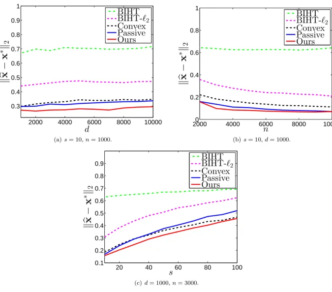
In this subsection, we will show our experimental results on general signals, i.e., no magnitude assumption guaranteed. The support of the signal vector is uniformly randomly selected from the entries, and the entry values are drawn from a standard normal distribution. The elements in the matrixUare also drawn from standard normal distribution and are independent from the signal x∗. We choose the noisy setting in [10] by flipping the signs of measurements with a probability of 0.1.
Figure 3.1(a) shows the recovery error against the dimensionality of signalsd. We can see that our proposed method outperforms all the other algorithms with a remarkable margin. As the dimensionality of signald goes up, the recovery error grows slowly, because the dependency ondis logarithmic by Theorem 3.4.11. We can also see that in this noisy setting, the more vulnerable BIHT and BIHT-`2 consistently perform worse than the other methods.
Figure 3.1(b) shows the recovery error against the number of measurementsn. Our method consistent-ly achieves the best performance. The passive algorithm also performs reasonabconsistent-ly well, but our method outperforms it in a wide range ofn.
Figure 3.1(c) shows the recovery error against the sparsity of signals s. We can see that for all the algorithms except BIHT, the error goes up quickly whensbecomes larger. Our algorithm is still consistently the best among all. Note that the dependency onsis not logarithmic, therefore, the error grows much faster than the case of varying d. We choose number of measurements n = 3000 here, which is larger than the signal dimensiond. This is practical in one-bit compressed sensing, because the one-bit measurements can be generated at very high rates. To sum up, our method can improve recovery accuracy in different parameter settings even with noise.
2000 4000 6000 8000 10000 0.3 0.4 0.5 0.6 0.7 0.8 0.9 1
d
k
b
x
−
x
∗k
2BIHT
BIHT-
`
2Convex
Passive
Ours
(a) s= 10,n= 1000. 20000 4000 6000 8000 10000 0.2 0.4 0.6 0.8 1n
k
b
x
−
x
∗k
2BIHT
BIHT-
`
2Convex
Passive
Ours
(b)s= 10,d= 1000. 20 40 60 80 100 0.1 0.2 0.3 0.4 0.5 0.6 0.7 0.8 0.9s
k
b
x
−
x
∗k
2BIHT
BIHT-
`
2Convex
Passive
Ours
(c)d= 1000,n= 3000.Figure 3.1: Recovery error for general signals
3.5.2
Approximate Vector Recovery for Strong Signals
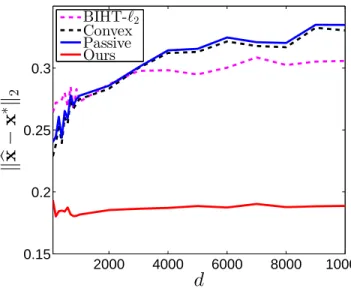
Now we present results of our recovery algorithm for strong signals. We will first generate unit sparse signals with random support, and set all nonzero entries to 1/√s. Noise is added in the same way with section 3.5.1. Figure 3.2 shows the recovery error of strong signals. According to Theorem 3.4.8, our error rate does not depend on dimensionalityd, which is verified by the results. Our recovery error stays on the same level, while the errors of all the other algorithms go up with increasing d. Note that the error of BIHT is much higher than the other algorithms. For better illustration and scaling the behavior of the other methods, we omit it in the figure here.
2000 4000 6000 8000 10000 0.15 0.2 0.25 0.3
d
k
b
x
−
x
∗k
2 BIHT-`2 Convex Passive OursFigure 3.2: Recovery error of strong signals againstdwhens= 10,n= 1000.
3.5.3
Support Recovery
We are now going to investigate the problem of support recovery. According to Theorem 3.4.3, our estimator enjoys oracle property for strong signals. We generate the signals in the same way as section 3.5.2 and present theF1score of support recovery in different dandn settings. F1 score is defined as the harmonic mean of precision and recall,
Precision = TP TP + FP, Recall = TP TP + FN, F1= 2·Precision·Recall Precision + Recall . where TP = d X i=1 1(xbi 6= 0,x∗i 6= 0), FP = d X i=1 1(xbi6= 0,x∗i = 0), TN = d X i=1 1(xbi = 0,x∗i = 0), FN = d X i=1 1(bxi= 0,x∗i 6= 0).
Note that our method is different from best previous work on support recovery. We do not need to construct specific measurement matrix as [5, 9], nor do we depend on dynamic range or adaption of the measurement process as [8]. Therefore, their methods are not directly comparable with ours.
Figure 3.3(a) shows the F1 score against signal dimension d. We can see that as the assumption in Theorem 3.4.3 is satisfied, our algorithm can achieve exact support recovery with very high probability. Our method and BIHT-`2 outperform the other algorithms with notable margins. In addition, Theorem 3.4.3
2000 4000 6000 8000 10000 0 0.2 0.4 0.6 0.8 1
d
F
1S
c
o
r
e
BIHT
BIHT-
`
2Convex
Passive
Ours
(a)s= 10,n= 1000. 2000 4000 6000 8000 10000 0 0.2 0.4 0.6 0.8 1n
F
1S
c
o
r
e
BIHT
BIHT-
`
2Convex
Passive
Ours
(b)s= 10,d= 1000.Figure 3.3: F1 score for support recovery
indicates that the support recovery of our method does not depend on d, which is also validated by the experiments. While for the other algorithms, the performance of the passive algorithm drops significantly asdgoes up; BIHT is not effective either, nor can it achieve a stable performance. Note that for the convex optimization method, there is no`0constraints on the signal. Therefore, most of the entries in the estimator are nonzero, resulting in very low precision. This explains the observation that convex optimization method always have a F1-score close to zero.
In Figure 3.3(b), we can find the F1 score against number of measurements n. For the same reason, the convex optimization method still suffers very low F1 score close to 0. For the other four methods, when there are not enough measurements, they perform poorly on support recovery. As the number of measurements goes up, the passive algorithm is the fatest to boost the performance. However, theF1score will stop increasing around 0.7 in spite of the increase of measurements. For BIHT, the performance is less stable, butF1score will still converge around 0.7 with increasing measurements. Compared with the passive algorithm, our algorithm needs a bit more measurements to converge in terms ofF1 score. Moreover, when n is larger than 500, our algorithm can achieve very good performance, almost recover the support with probability 1. BIHT-`2has a similar behavior as our algorithm with enough measurements, but our method requires fewer measurements.
3.5.4
Oracle Property
We will further study the oracle property of our estimator. We plot the difference between proposed estimator and the oracle estimator in (3.4.1). By Theorem 3.4.3, the two should be the same with high probability. In
2000 4000 6000 8000 10000 0 0.2 0.4 0.6 0.8 1
n
k
b
x
−
b
x
O
k
2
BIHT
BIHT-
`
2Convex
Passive
Ours
Figure 3.4: Difference between estimators and oracle estimators againstnwhens= 10,d= 1000.
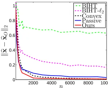
Figure 3.4, we can see that when the number of measurements goes up, the difference between our estimator and oracle estimator converges to zero very quickly. For BIHT and BIHT-`2, the differences are large; for the passive algorithm, the difference is still discernable, and the support recovery is not satisfying; for the convex optimization algorithm, although the norm of the difference is converging, it cannot recover the support. Therefore, our estimator is the only one that enjoys oracle property.
3.6
Summary
We proposed a novel algorithm [14] for the problem of one-bit compressed sensing, which is able to achieve both vector recovery and support recovery with strong theoretical guarantees. We introduce the nonconvex sparsity-inducing penalty functions to this problem for the first time.
More specifically, our main contributions are summarized as follows:
• We propose to incorporate sparsity-inducing penalty functions into one-bit compressed sensing, and derive an algorithm to efficiently solve the resulting problem. To the best of our knowledge, this is the first work on one-bit compressed sensing that utilizes nonconvex penalty functions.
• We prove that our proposed method improves sample complexity from previous best resultsO(slogd/2) to O(s/2) for strong signals. And for general signals, our algorithm attains a sample complexity be-tween O(slogd/2) andO(s/2).