ALGORITHM-LEVEL OPTIMIZATIONS FOR SCALABLE PARALLEL GRAPH PROCESSING
A Dissertation by
HARSHVARDHAN
Submitted to the Office of Graduate and Professional Studies of Texas A&M University
in partial fulfillment of the requirements for the degree of DOCTOR OF PHILOSOPHY
Chair of Committee, Nancy M. Amato Co-Chair of Committee, Lawrence Rauchwerger Committee Members, Anxiao (Andrew) Jiang
Marvin L. Adams Head of Department, Dilma Da Silva
May 2018
Major Subject: Computer Science
ABSTRACT
Efficiently processing large graphs is challenging, since parallel graph algorithms suffer from poor scalability and performance due to many factors, including heavy communication and load-imbalance. Furthermore, it is difficult to express graph algorithms, as users need to understand and effectively utilize the underlying execution of the algorithm on the distributed system. The performance of graph algorithms depends not only on the characteristics of the system (such as latency, available RAM, etc.), but also on the characteristics of the input graph (small-world scale-free, mesh, long-diameter, etc.), and characteristics of the algorithm (sparse computation vs. dense communication). The best execution strategy, therefore, often heavily depends on the combination of input graph, system and algorithm.
Fine-grained expression exposes maximum parallelism in the algorithm and allows the user to concentrate on a single vertex, making it easier to express parallel graph algorithms. However, this often loses information about the machine, making it difficult to extract performance and scalability from fine-grained algorithms.
To address these issues, we present a model for expressing parallel graph algorithms using a fine-grained expression. Our model decouples the algorithm-writer from the underlying details of the system, graph, and execution and tuning of the algorithm. We also present various graph paradigms that optimize the execution of graph algorithms for various types of input graphs and systems. We show our model is general enough to allow graph algorithms to use the various graph paradigms for the best/fastest execution, and demonstrate good performance and scalability for various different graphs, algorithms, and systems to 100,000+ cores.
DEDICATION
To my Mother and Father, who inspired by example, encouraged and supported me, and inculcated in me dedication, strong ethics and morals.
ACKNOWLEDGMENTS
I would like to thank my advisers, Prof. Nancy Amato and Prof. Lawrence Rauchwerger for their continued mentoring, support and guidance throughout my undergraduate and graduate career. I would like to thank my committee members Prof. Andrew Jiang and Prof. Marvin Adams for their mentorship and guidance.
Special thanks to Adam Fidel, Dr. Gabriel Tanase, Antal Buss, Dr. Ioannis Papadopoulos, Glen Hordemann, Brandon West and Mani Zandifar for not only being excellent colleagues and lab-mates, but also close friends throughout my time in graduate school. Finally, I would like to thank Dr. Timmie Smith and Dr. Nathan Thomas, and the members of the Parasol Lab for all their help and collaboration.
CONTRIBUTORS AND FUNDING SOURCES
Contributors
This work was supported by a dissertation committee consisting of Professors Nancy M. Am-ato [advisor], Lawrence Rauchwerger [advisor] and Anxiao Jiang of the Department of Computer Science and Engineering, and Professor Marvin L. Adams of the Department of Nuclear Engineer-ing.
Portions of this research were previously published. The basic framework was presented as The STAPL Parallel Graph Library in the proceedings of the 25th International Workshop on Languages and Compilers for Parallel Computing (LCPC) [1]. The k-level-async paradigm was published in the proceedings of the 23rd International Conference on Parallel Architectures and Compilation Techniques (PACT) [2], where it won the Best Paper Award. The techniques for com-munication reduction in graph algorithms were published as An Algorithmic Approach to Com-munication Reduction in Parallel Graph Algorithms in the proceedings of the 24th International Conference on Parallel Architectures and Compilation Techniques (PACT) [3], where it was a Best Paper Award Finalist. The techniques for processing big data graphs were published as A Hybrid Approach to Processing Big Data Graphs on Memory-Restricted Systems in the proceedings of the 29th IEEE International Parallel and Distributed Processing Symposium (IPDPS) [4]. All work for the dissertation was completed in collaboration with the co-authors of the aforementioned works.
Funding Sources
This research is supported in part by NSF awards CCF 0702765, CNS-0551685, CCF-0833199, CCF-1439145, CCF1423111, CCF-0830753, IIS-0917266, by DOE awards DEAC02-06CH11357, DE-NA0002376, B575363, by Samsung, IBM, Intel, and by Award KUS-C1-016-04, made by King Abdullah University of Science and Technology (KAUST). This research used resources of the National Energy Research Scientific Computing Center, which is supported by the Office of Science of the U.S. Dept. of Energy under Contract No. DE-AC02-05CH11231.
TABLE OF CONTENTS
Page
ABSTRACT . . . ii
DEDICATION . . . iii
ACKNOWLEDGMENTS . . . iv
CONTRIBUTORS AND FUNDING SOURCES . . . v
TABLE OF CONTENTS . . . vi
LIST OF FIGURES . . . ix
LIST OF TABLES. . . xiii
1. INTRODUCTION . . . 1
1.1 Contributions . . . 2
1.2 Overview of Our Approach . . . 4
1.3 Outline . . . 5
2. THE STAPL GL MODEL . . . 7
2.1 Related Work . . . 8
2.1.1 Existing Models . . . 8
2.1.2 Other Graph-Processing Systems . . . 9
2.2 The Fine-Grained Graph Processing Paradigm . . . 10
2.2.1 PageRank and Other Algorithms . . . 12
2.3 The Hierarchical Graph Processing Paradigm . . . 13
2.3.1 Graph Hierarchies . . . 15
2.3.2 Hierarchical Operators . . . 16
2.3.3 Creating The Hierarchy . . . 17
2.3.4 Analysis of Cost of Hierarchy Creation . . . 17
2.3.5 Algorithms Using the Hierarchical Paradigm . . . 19
3. THE KLA GRAPH PARADIGM – PROCESSING GRAPHS WITH BOUNDED ASYN-CHRONY . . . 22
3.1 Existing BSP and Asynchronous paradigms . . . 22
3.1.1 Tradeoffs: Asynchronous vs. BSP . . . 23
3.3 Requirements, Guarantees and Proof of Correctness . . . 24
3.4 Finding optimal-k . . . 25
3.4.1 Adaptive KLA . . . 26
3.4.2 A Model for Approximating
k
opt. . . 274. COMMUNICATION REDUCTION OPTIMIZATION – FOR SMALL-WORLD SCALE-FREE GRAPHS . . . 32
4.1 Out-degree and in-degree optimizations . . . 33
4.2 Hierarchical model . . . 34
4.2.1 Locality-Based Communication Optimization . . . 34
4.2.2 Creating in-degree hierarchy . . . 35
4.2.3 Distributed Hubs Optimization . . . 36
4.2.4 Using the hierarchy . . . 39
4.3 Analysis. . . 39
4.3.1 Communication Volume . . . 40
4.3.2 Space Overhead . . . 41
4.4 Implementation . . . 42
4.5 Related Work . . . 42
5. OUT-OF-CORE GRAPH PROCESSING . . . 46
5.1 Introduction. . . 47
5.2 Graph Storage . . . 48
5.3 Processing Out-of-Core Graphs . . . 49
5.4 Optimizations To Reduce Disk I/O . . . 52
5.5 Analysis of I/O Costs . . . 54
5.6 Implementation . . . 55
5.7 Related Work . . . 56
5.8 Conclusion. . . 57
6. APPLICATIONS OF GRAPH PROCESSING . . . 58
6.1 Motion Planning. . . 58
6.2 Nuclear Particle Transport . . . 59
6.3 Seismic Ray-Tracing . . . 64
6.4 Conclusion. . . 64
7. IMPLEMENTATION . . . 65
7.1 ThePGRAPH PCONTAINER. . . 65
7.2 Graph Traversal Strategies . . . 68
8. RESULTS . . . 71
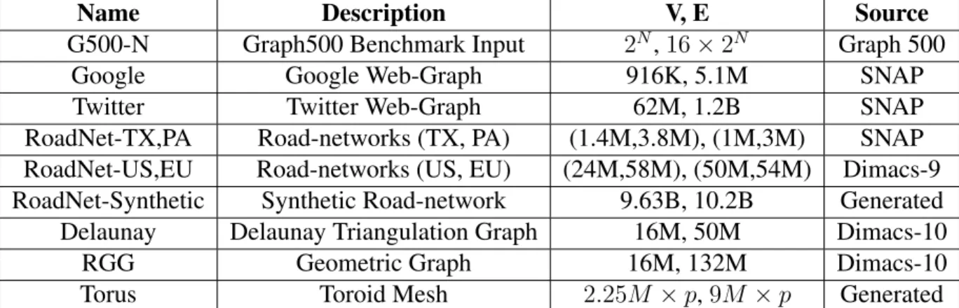
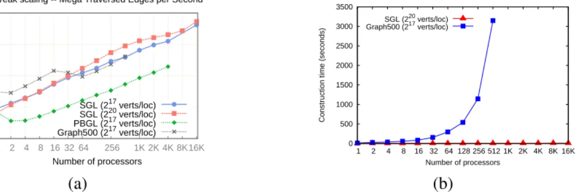
8.1 Experimental Setup and Input Graphs . . . 71
8.3 Comparison with in-memory libraries . . . 73
8.4 KLA Experiments . . . 75
8.4.1 Level-Synchronous vs. Asynchronous BFS . . . 76
8.5 Evaluation of KLA BFS . . . 76
8.6 Evaluation of Adaptive KLA BFS. . . 79
8.7 Evaluation of Other Types of Algorithms . . . 80
8.8 KLA with Other Graph Frameworks . . . 81
8.9 Hierarchical Communication Reduction . . . 83
8.9.1 Improving Work Imbalance . . . 83
8.9.2 Applications . . . 83
8.9.3 Fundamental Algorithms . . . 86
8.9.4 Graph Mining Algorithms . . . 87
8.9.5 Application of Traversals . . . 88
8.9.6 Other Graphs. . . 90
8.9.7 Overhead of Hierarchy Creation . . . 92
8.10 Out-of-Core Performance . . . 94
9. SUMMARY . . . 101
LIST OF FIGURES
FIGURE Page
2.1 The fine-grained BFS algorithm. . . 12
2.2 Pseudocode for the graph paradigm (level-sync execution). . . 13
2.3 The PageRank algorithm. . . 13
2.4 Thek-core algorithm. . . 14
2.5 Specification of a hierarchical algorithm. . . 16
2.6 Pseudocode for the hierarchical graph paradigm. . . 18
3.1 Visitation logic for async, KLA and level-sync behavior of BFS. . . 24
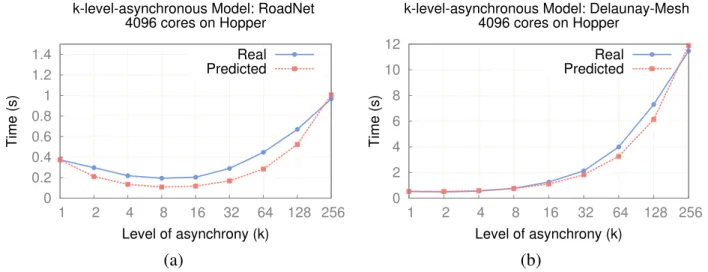
3.2 KLA Model: predicted vs. actual execution times on HOPPERfor a BFS. . . 31
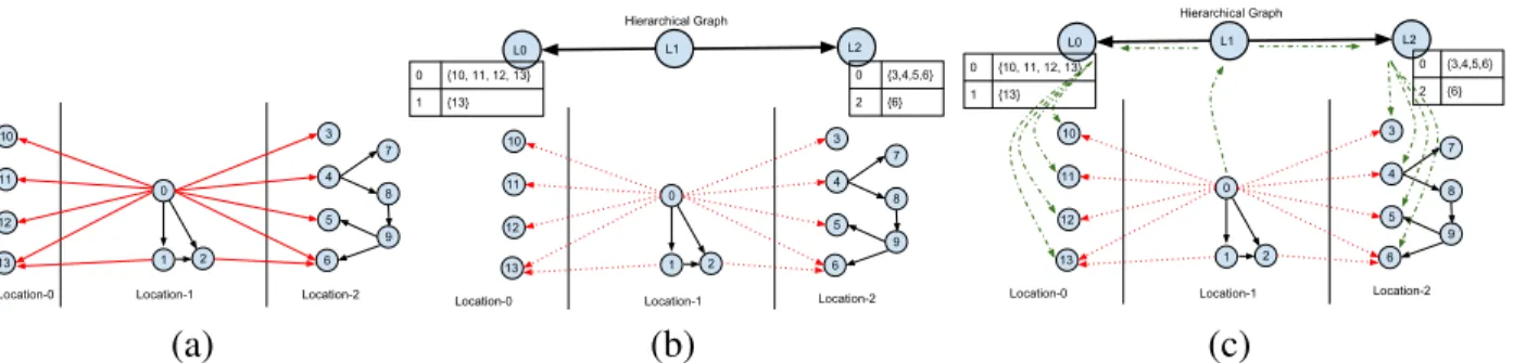
4.1 Creating a hierarchy: (a) A flat graph, with remote, inter-partition edges (red lines) and (b) its hierarchical representation with metadata. Using the hierarchy: (c) Remote communication during algorithm execution (shown in green). Hierarchical graph replaces inter-partition edges in original graph (red dashed-lines represent deleted edges) with a single super-edge between each partition (solid black lines on top-level graph). Generalizable to multiple levels of machine hierarchy. . . 35
5.1 Diagram of the storage paradigm with two subgraphs in memory and two sub-graphs on disk. An update on a loaded vertex is being applied in memory while an update to an un-loaded vertex is being stored in the pending updates shard. . . 49
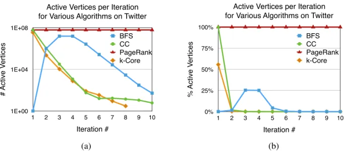
5.2 Variation in active vertices in the first ten iterations of various algorithms on the Twitter graph, shown as (a) count on log-scale, and (b) percentage of total vertices. . 51
5.3 Pseudocode for the off-core graph paradigm.. . . 52
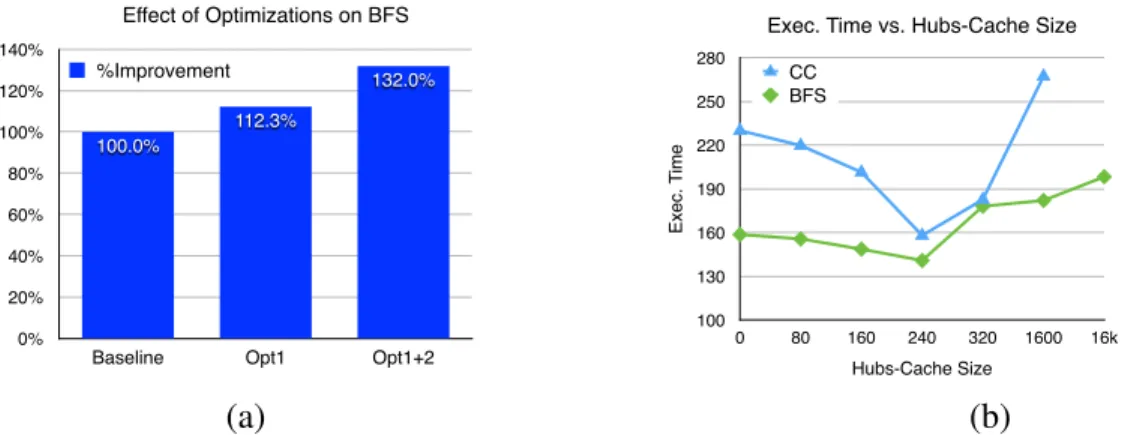
5.4 Effects of optimizations on performance: (a) Skipping inactive subgraphs (Opt1) and inactive vertices (Opt2), (b) Effect of varying size of hubs-cache for BFS and connected components (CC). Both plots run on Graph 500 input graph with 16 million vertices and 256 million edges, on a PC with 4GB RAM. . . 54
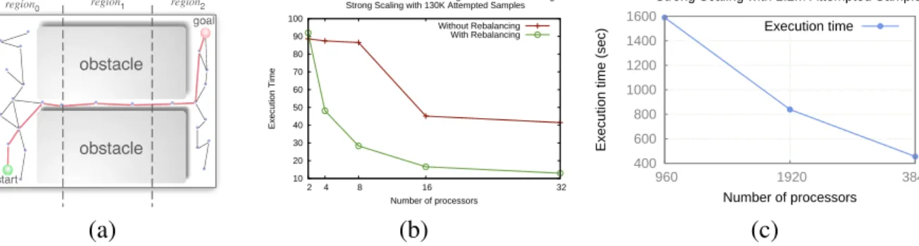
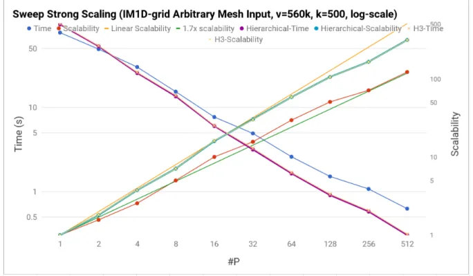
6.1 Strong scaling for a parallel motion planning application on a poorly balanced envi-ronment (a) with and without rebalancing techniques (b), at scale with rebalancing (c). . . 59 6.2 Strong scaling of parallel multi-sweep (hierarchical and non-hierarchical) on an
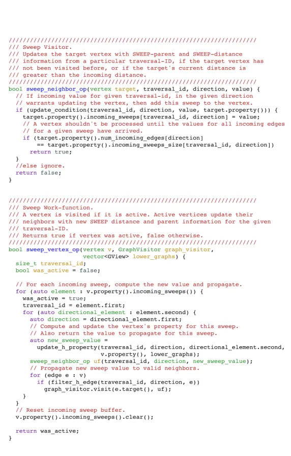
IM1D-Grid Arbitrary Mesh Input, with 560k vertices on a Cray XK6 machine. . . 60 6.3 Pseudocode for internal methods of the hierarchical parallel multi-sweep. . . 61 6.4 Pseudocode for vertex- and neighbor- operators for the hierarchical parallel
multi-sweep.. . . 62 6.5 Pseudocode for the hierarchical parallel multi-sweep, along with the driver for the
sweep.. . . 63 7.1 Internal base-class implementation ofapply_asyncmethod illustrating address
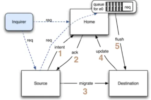
resolution. . . 67 7.2 Asynchronous migration protocol forPGRAPH.. . . 67 7.3 (a) The fine-grained BFS algorithm, with (b) BFS vertex operator and (c) BFS
visitor operator. Also shows how changing the visit-functions between level-sync (d), async (f) and k-level-async (e) visit functions changes the behavior of the algorithm from async to KLA to level-sync, using BFS as an example algorithm. . . 70 8.1 Comparison of MTEPS (a) and construction times (b) for PGRAPH, PBGL and
Graph 500 ref. implementation. Note log-scale y-axis for (a) . . . 73 8.2 Execution times of Graph500 on various graph libraries normalized to STAPL GL
on CRAY XE6m. Shared-memory graph libraries (Galois, GreenMarl) are shown to 16 cores. . . 74 8.3 Weak scaling ofSTAPL GL on the Graph500 benchmark input on CRAY XE6 with
220vertices per core. Y-axis shows throughput in Mega-Traversed Edges per Sec-ond (MTEPS) in log-scale. . . 75 8.4 Scalability (Throughput) of BFS on (a) Graph500 benchmark (max.|V|=16B,|E|=256B)
and (b) torus (max.|V|=9.2B,|E|=37B). . . 75 8.5 Modeling KLA: Study of effects of graph diameter on the optimalkparameter. . . 77 8.6 Performance of KLA BFS on road networks for (a) TX, PA and (b) USA on HOPPER. 78
8.7 Performance of KLA vs. Level-Sync BFS on synthetic road network, 98,304 cores on HOPPER. . . 78
8.8 KLA BFS speedup withkopt and Adaptive KLA on various graphs on HOPPER. . . 79
8.9 Evaluation ofk-core PageRank and SSSP on 16,384 cores on HOPPER. . . 81
8.10 Nested KLA with Green-Marl for (a) PageRank and (b) conductance, up to 24,000 cores. . . 82 8.11 Speedup of KLA BFS in Galois on various graphs relative to the fastest version of
Galois (bulk synchronous or asynchronous) on HOPPER. . . 82
8.12 Comparison of work-imbalance (number of edges) for flat and hierarchical graphs for Graph500 inputs (weak-scaling) on a CRAY XE6m, along with trendlines showing growth rates. . . 84 8.13 Throughput of (a) BFS, (b) connected components and (c) PageRank on
Watts-Strogatz input on BGQ,131,072 cores. At scale, the hierarchical approach has an improvement of 1.59x, 1.78x and 1.64x over the flat approach, respectively. . . 84 8.14 Scalability (Throughput, log-scale) of various algorithms using hierarchical
ap-proach. Graph500 input graph with 4 billion vertices and 64 billion edges at12,288 cores. . . 85 8.15 Communication reduction using hierarchical approach and (b) Scalability
(Through-put) of BFS on Graph500 benchmark. . . 86 8.16 Communication reduction using hierarchical approach and (b) Scalability
(Through-put) of Connected Components on Graph500 input. . . 87 8.17 Communication reduction using hierarchical approach and (b) Scalability
(Through-put) of PageRank on the Graph500 input graph. . . 89 8.18 Communication reduction using hierarchical approach and (b) Scalability
(Through-put) of k-core on Graph500 input. . . 89 8.19 Throughput of Betweenness Centrality (BC), Pseudo-Diameter (PD), and
Commu-nity Detection (CD) on Graph500. . . 90 8.20 Running times of BFS on various input graphs using flat and hierarchical
ap-proaches. . . 92 8.21 Improvement of the hierarchical approach on BFS for varying rewiring-probability
of a Watts-Strogatz graph. . . 92 8.22 Comparison of total construction times of flat and hierarchical graphs for various
inputs. . . 93 8.23 Comparison of graph construction and algorithm execution times of flat and
8.24 STAPL GLrunning time (various algorithms) vs. GraphChi on the Graph500 bench-mark input with16million vertices,256million edges, running on PC with (a) 4GB RAM and (b) 16GB RAM. . . 97 8.25 Breakdown of times for different phases (loading, storing and processing) for (a)
BFS and (b) PageRank with respect to memory size. . . 97 8.26 STAPL GLrunning time (various algorithms) on the Graph500 benchmark input on
an Android tablet with 1GB RAM,4million vertices,64million edges. . . 98 8.27 STAPL GL running time for BFS, PageRank (PR) and connected components (CC)
on the Twitter input on multiple nodes of Cray XE6. . . 98 8.28 STAPL GLrunning time (various algorithms) on 4GB PC on the Twitter graph with
65million vertices, 1.2 billion edges, and the Friendster graph with 118 million vertices,2.6billion edges. . . 99 8.29 STAPL GL running time across platforms on the Graph500 input graph with 16
million vertices,256million edges. . . 99 8.30 STAPL GLrunning time across platforms on the Twitter input graph with65million
LIST OF TABLES
TABLE Page
1. INTRODUCTION
Processing large graphs is essential in a variety of domains, from social network and web-scale graphs to scientific meshes and nuclear reactor-design [5]. Processing these graphs in a reason-able time usually requires parallelism. Using a distributed data-structure allows massive graphs to be processed quickly and concurrently. However, parallelizing graph algorithms efficiently is a challenging problem that has received significant attention for several decades [6]. Despite many attempts over the past decade [7, 8, 9] to allow programmers to easily express their graph compu-tations in parallel, graph algorithms remain notoriously hard to scalably parallelize. Existing graph libraries are restrictive in allowing users to express algorithms and may require them to manage details of data-distribution and communication. Developers also often correlate an increase in the level of abstraction with a corresponding decrease in performance. Vice-versa, most highly-optimized implementations tend to introduce system/parallelism details in the algorithm, thereby decreasing the level of abstraction. Furthermore, the performance of many parallel graph algo-rithms tend to heavily depend not only on the system characteristics, but also on the characteristics of the input graph. For example, a breadth-first search on a binary-tree has significantly different performance characteristics from the same algorithm on a social-network.
In particular, graph algorithms suffer from poor scalability and performance at scale due to poor work balance (both, among processors and across supersteps of execution of the algorithm), heavy communication, and irregular access. These bottlenecks manifest due to the combination of the graph, algorithm and the system. For example, given an input graph, the PageRank algorithm ex-hibits heavier communication than a breadth-first traversal. Conversely, though, PageRank, where all supersteps process every vertex, displays a more balanced computational pattern across the supersteps of the algorithm than breadth-first traversal, where some supersteps may process the majority of the graph, while other levels only process small percentage of vertices.
Similarly, changing input graphs from uniform or semi-uniform mesh networks used in scien-tific computations and simulations, to small-world scale-free graphs representing social and web
networks, has a dramatic impact on the execution of the algorithm. For the same algorithm, a scale-free network will produce dense communication to almost every processor due to the presence of
hub-verticesthat have very high out-degrees. The small-world property will result in the majority
of vertices being processed in a few supersteps. The challenge in such graphs is to improve the effective bandwidth of the system, as well as improve the load-balance in order efficiently process the hub vertices and their connections. A mesh network, on the other hand, may typically have a large diameter and low variance in the vertex degree. This combination results in a very large number of supersteps, each with only a small fraction of the total work. The challenge here is to improve latency and reduce the cost of global synchronizations, in order to address the large num-ber of supersteps. Existing frameworks such as Google’s Pregel [9] or the Parallel Boost Graph Library (PBGL) [7] can only effectively solve certain limited subsets of these combinations, and suffer from poor performance in other cases. Other libraries, such as Galois [10], Ligra [11] and MTGL [8] are limited to shared-memory, and are therefore limited in the scale of the problem they can solve. There doesn’t exist a framework that can address all these challenges at large-scale.
Another instance where these bottlenecks become prohibitive is out-of-core graph processing. Reading from and writing to disks are high-latency operations. Due to the irregular nature of graph access-patterns, conventional techniques of paging and prefetching do little to alleviate the latency. The best available out-of-core graph processing systems still require O(N2) random reads and writes [12], and consequently are unable to perform well at scale.
1.1 Contributions
This research designs a generic parallel graph library (STAPL GL) that allows users to
concen-trate on graph algorithm development by abstracting them from the input data and the details of the underlying distributed environment, while providing portable, scalable performance. STAPL GL
allows for the separation of the algorithm from the container, as well as decouples the algorithm from the input graph and machine through the use of traversal strategies. It provides a generic, cus-tomizable graph container, a collection of common parallel graph algorithms, as well as multiple graph traversal strategies (including level-synchronous, asynchronous and hierarchical). Further,
STAPL GL automates load balancing and locality-related optimizations. Specific contributions of this research include:
• Programmability and Abstraction. Provide a high-level graph abstraction to allow
pro-grammers to completely decouple the design of the graph algorithm from the details of par-allelism, input graph, implementation of the graph container and the machine. Users express their computation in its most natural form, while the underlying data-structure implementa-tion and traversal strategy can be chosen to offer maximum performance based on the input graph and platform.
• Multiple Graph Traversal Strategies. Provide multiple traversal strategies for expressing
graph algorithms to allow the algorithms to achieve the best performance for different classes of input graphs and machines. In particular, this research will focus on the following traversal strategies:
– KLA(k-level Asynchronous). This novel traversal strategy unifies asynchronous and
level-synchronous traversal strategies, while allowing parametric control of asynchrony. We also provide a model to estimate the appropriate level of asynchrony for a given in-put graph, a strategy to adaptively determine k, and show how to transform common asynchronous and level-synchronous graph algorithms to KLA.
– Hierarchical Traversal Strategy.This traversal strategy allows users to express
com-putations hierarchically. It also allows expression of certain algorithms (e.g. graph-partitioning and Boruvka’s minimum spanning-tree) in their most natural form, as well as allows for reduction of communication in certain cases by taking advantage of the machine hierarchy.
– Out-of-Core Strategy.This strategy uses sub-graph paging together with the
asynchronous-push model to eliminate non-sequential reads and minimize writes, making it suitable for out-of-core processing. A theoretical model shows the I/O to be linear in the
num-ber of reads and writes, improving on the existingO(n2)strategies. This translates to a10×improvement in real-world performance.
• Scalable Performance. Provide improved scalability in performance and data size over
tens of thousands of cores compared with existing graph libraries on standard benchmarks. Moreover, provide light-weight support for load balancing through asynchronous data mi-gration, and demonstrate improved performance and scalability in a real-world production application by mitigating load-imbalance through automatic redistribution of vertices. An implementation of the STAPL Parallel Graph Library infrastructure[1] provides a parallel graph container (PGRAPH), associated graph PVIEWS, common graph algorithms, as well as the k-level-async, hierarchical, and out-of-core processing strategies. Results show improved per-formance over existing graph libraries and frameworks, and scalability to 100,000+ cores. Ex-periments with k-async show substantial performance improvements over existing level-synchronous and alevel-synchronous traversal strategies, while the hierarchical and out-of-core strate-gies show an order-of-magnitude improvement in performance over flat graph processing and other out-of-core graph processing strategies respectively.
1.2 Overview of Our Approach
We provide a graph-processing engine (thegraph_paradigm) to control the execution of algo-rithms, that can effectively utilize available resources for fast, scalable processing of graphs. To do this, we allow users to express their algorithms in a vertex-centric fine-grained manner that abstracts them from details of parallelism and exposes the maximum amount of parallelism avail-able in the algorithm. The graph algorithms themselves do not change and are decoupled from execution policies (distributed/shared, disk/in-memory, etc.), allowing the execution strategies to change, without changing the algorithm.
We further provide multiple strategies of algorithm execution for tolerating high-latencies and low bandwidths in multiple situations. The k-Level asynchronous paradigm allows latency-hiding in high-latency systems by trading- off costly global barriers for point-to-point local
synchroniza-tions and redundant work. The hierarchical paradigm increases effective bandwidth by minimizing the amount of communication, and the out-of-core processing paradigm uses sub-graph paging with the asynchronous push-model to eliminate non-sequential reads and minimize writes.
Much of our research was previously published. The overall framework design and imple-mentation was published at theInternational Workshop on Languages and Compilers in Parallel
Computing(LCPC) 2012 [1]. Thek-level-asynchronous paradigm for unifying existing BSP and
asynchronous paradigms was published at theInternational Conference on Parallel Architectures
and Compilation Techniques (PACT) 2014 [2], and won the Best Paper Award. The work on
out-of-core graph processing was published at theIEEE International Parallel & Distributed
Pro-cessing Symposium(IPDPS) 2015 [4]. Finally, the work on hierarchical communication reduction
in graph algorithms was published at theInternational Conference on Parallel Architectures and
Compilation Techniques(PACT) 2015 [3], and was nominated for the Best Paper Award.
1.3 Outline
This dissertation is organized as follows. Section 2 begins with an overview of the STAPL GL model, followed by a brief discussion of existing graph processing models and systems, and
tradeoffs involved with each. The section then describes the asynchronous push model and how various graph algorithms may be expressed in this model.
Section 3 describes the two existing approaches to processing graphs – Bulk Synchronous Parallel (BSP) and Asynchronous – and discusses the tradeoffs involved in using them. It then introduces a novel paradigm for graph processing – thek-Level Asynchronous paradigm (KLA), that unifies the two existing approaches, along with requirements, guarantees and a proof of cor-rectness. It further describes two approaches for finding the optimal level of asynchrony for a given combination of input graph, algorithm, and system.
Section 4 presents an approach to reducing the amount of communication done in a graph processing system, and shows how it can improve the performance of algorithms on small-world scale-free networks. It then analyses bounds on the amount of communication reduction and the space overhead required. Finally, it concludes with a discussion of related work.
Section 5 introduces the problem of out-of-core graph processing, including the challenges in-volved in processing large graphs from disk. It then presents a novel approach for scalably and efficiently processing out-of-core graphs on a distributed machine, along with several optimiza-tions to reduce the disk I/O. The approach elliminates non-sequential disk reads and minimizes random disk writes. The section next analyss the I/O costs associated with processing graphs in this paradigm, and concludes with a brief discussion of the related work.
Section 6 provides an overview of real-world applications from different domains built using
STAPL GL. Details of an implementation of STAPL GL in STAPL, along with the various graph processing paradigms are provided in Section 7, and results of experimental evaluation of this implementation is provided in Section 8. Section 8 also provides an overview of the experimental setup and input graphs used, along with comparisons with existing graph processing systems. It then provides detailed evaluation of each of the different graph processing paradigms at large scale for various input graphs and algorithms on different systems.
2. THE STAPL GL MODEL
One of the challenges to processing graphs is the difficulty in expressing parallel graph algo-rithms naturally and effectively. To overcome this,STAPL GLuses differentmodelsto decouple the algorithm’s expression from its execution, abstracting away the parallelism and communication details. Graph algorithms in STAPL-GL are expressed using either a fine-grained vertex-centric manner, or a coarse-grained hierarchical manner.
The fine-grained “vertex-centric” approach, popularized by the Pregel graph processing frame-work [9], is suitable for expressing a large class of graph algorithms such as breadth-first search (and other traversals), PageRank, connected components, k-core decomposition, centrality metrics, and coloring. Several existing graph processing frameworks use a vertex-centric model to express algorithms. Algorithm writers specify operations to be performed on vertices and their neighbors, which are iteratively applied to the vertices of the graph by the execution engine to execute the algorithm.
However, there is a class of naturally hierarchical graph algorithms such as Boruvka’s mini-mum spanning trees, graph partitioning, and agglomerative clustering, for which the vertex-centric approach is not effective. Due to their inherent hierarchical nature and the need to operate on coarse chunks of the graph instead of individual vertices, the fine-grained approach makes it hard for al-gorithm developers to express such alal-gorithms. On the other hand, coarse graph alal-gorithms are harder to express on a parallel system and limit the amount of parallelism exposed – a fine-grained algorithm exposes the maximum amount of parallelism as each unit of work can be independently processed in parallel. To address this,STAPL GLalso provides a hierarchical model that eliminates the need for the algorithm writer to think about the details of creating the hierarchy itself, providing instead well-specified operators that define the hierarchy, executing the algorithm as the hierarchy is built.
This chapter starts with a discussion of relevant related work in this area, along with existing ap-proaches of expressing graph algorithms and their tradeoffs. Section 2.2 describes the fine-grained
graph paradigm in STAPL GL, along with example algorithms. Finally, Section 2.3 describes the hierarchical (coarse-grained) paradigm inSTAPL GL, and how algorithms are expressed in it.
2.1 Related Work
2.1.1 Existing Models
Pull vs. Push Model. Graph algorithms typically exchange data between the vertices of the
graph. This may be done by “pushing” the current state of a vertex to a subset of its neighbors, or “pulling” (or reading from) the current state of its neighboring vertices. Systems such as Pregel [9] and SGL rely on the push model, while GraphLab [13] and GraphChi [12] rely on the pull model of communication. While both methods produce the same end result, the push model can be implemented asynchronously, by allowing overlapped communication and computation – a vertex can send its state to its neighbors and then perform local computation. On the other hand, the pull model needs to be synchronous. Furthermore, since in most graph algorithms vertices do not communicate with all their neighbors (and only a small subset of total vertices are actively communicating at all in each iteration), it may not be possible for a vertex to know which subset of its neighbors (if any) to pull data from, and therefore, systems implementing the pull model must read the states of all neighboring vertices at every step. The push model only needs to communicate data that is required, allowing the algorithm to perform much lower communication than in the pull model. Push models are also more naturally suited for distributed-memory computation than pull models. Due to these reasons, we chose to use a push model for our system. We show comparisons in scalability and speed between implementations of the two models in our experiments section.
Vertex vs. Edge Centric Models. Another way to classify fine-grained graph models is whether
they emphasize computations upon vertices or edges. Vertex-centric models incorporate the “think like a vertex” [9] philosophy, where the algorithm is expressed in terms of operations on vertices and their associated states (including any associated outgoing-edge states), and the edges are used to establish communication between vertices. Operations read and update vertex states, perform computations on these vertices, and send the result of the computations to neighboring vertices.
On the other hand, edge-centric algorithms are expressed in terms of operations on edges, with associated source- and target-vertex states. Edge-centric operators read states from both, source and target vertices of an edge, and perform computations to update their states. For certain al-gorithm, an edge-centric approach may provide a more natural expression than a vertex-centric model. However, since multiple edges may be incident upon the same vertex, a coherence mech-anism is required to keep the vertex’s state consistent while potentially multiple parallel updates read from and write to the same vertex. This, in practice limits the scalability of edge-centric models, making them harder to implement efficiently on distributed systems.
Coarse-Grained Models. There has also been work in expressing parallel graph algorithms in
a coarse-grained manner. Such models are subgraph-centric, where the graph is partitioned into subgraphs and some computation is performed on them, followed by an exchange of boundary data between the subgraphs. Certain algorithms such as Boruvka’s MST, graph partitioning and clus-tering are naturally hierarchical, and are therefore also better expressed in such models. However, non-hierarchical algorithms such as traversals, PageRank, and several others, are better expressed in fine-grained models which do not require a separate specification of the boudary condition.
2.1.2 Other Graph-Processing Systems
The Parallel Boost Graph Library (PBGL) [7] is a stand-alone distributed-memory graph library,
with similar goals asSTAPL GL. An important difference fromSTAPL GLis that sincePBGL does
not provide a shared-object view, it exposes users to explicit knowledge of parallelism and data distribution details through the use of process groups. This makes it more difficult to program. As an example, PBGL’s interface requires the user to know explicitly the location of a vertex before any operations may be performed on it, and therefore, there is no locality-agnostic way to access remote vertices. Another difference is thatPBGL’s algorithms are inherently level-synchronous.
The Multi-Threaded Graph Library (MTGL) [8] is a shared-memory graph library designed to effectively utilize the unique architectural features of Cray XMP massively multithreaded ma-chines. It can be ported to other platforms using the QThreads library. However, the model exposes programmers to the QThreads API, as well as the details of multi-threaded programming.
Google’s Pregel [9] is a library for processing graphs in parallel that emphasizes vertex-centric computation and algorithm design, making it easy to express and versatile. Pregel uses the Bulk Synchronous Processing (BSP) computational model [14] for executing algorithms.
GraphLab/PowerGraph [13] is a distributed-memory graph framework that allows users to choose between synchronous and asynchronous execution at runtime, but it does not support para-metric control of asynchrony. It uses a pull-model (gather/scatter approach) to express compu-tations. However, this model impacts scalability on large parallel systems, and may incur extra communication. It also requires users to understand low-level details of parallelism such as mem-ory consistency and concurrency, as they have to choose a consistency model for their application and understand its implications.
There are also edge-centric graph processing systems such as Ligra [11], which express al-gorithms on edges, rather than the more commonly used vertex-centric model. However, due to the need for maintaining coherence among vertices, edge-centric libraries are limited to shared-memory systems in practice, and there doesn’t exist a practical distributed-shared-memory implementation of this paradigm.
GoFFish is a subgraph-centric graph processing framework for large-scale graph analytics. This framework aims to address scalability bottlenecks in fine-grained models by exposing par-tition information of the input graph to the algorithm writer. While this allows for performance and locality-based optimizations such as reduced communication and reduced number of super-steps, it makes the algorithm harder to express, since the user has to understand and account for data-distribution and graph partitioning. STAPL GL’s fine-grained model overcomes challenges of scalability by optimizing communication separately from the user’s expression of the algorithm. This allowsSTAPL GLalgorithms to be expressible and scalable.
2.2 The Fine-Grained Graph Processing Paradigm
Fine-grained vertex-centric algorithms in STAPL GL use an asynchronous push-update model, which exposes a large amount of parallelism, while allowing the most flexibility in choosing ex-ecution and communication strategies based on input and system. In this section, we show how
an example algorithm, breadth-first traversal (BFS) (Figure 2.1) can be expressed in STAPL GL’s fine-grained graph paradigm. Other algorithms such as connected components,k-core, PageRank, community detection, graph coloring, betweenness centrality, pseudo-diameter, etc. can also be expressed in a similar manner.
Breadth-first traversal (BFS) is an important graph algorithm due to its extensive usage in traversing graphs, and due to its indirect usage as a part of numerous other graph algorithms, such as betweenness centrality. A BFS of a graph marks each of its vertices with their distance from a given source vertex.
To express an algorithm, the user provides two operators – a vertex-operator (Figure 2.1(a)) which performs the computation of the algorithm locally on a single vertex, and a
neighbor-operator (Figure 2.1(b)) that updates the neighbor-vertices of the source vertex with the results
of the computation based on incoming values from active vertices or edges. The user can option-ally also provide an edge-operator to perform local computation on adjacent edges of a vertex based on values passed-in from the source vertex. The edge-operator is mostly needed when the algorithm sends different data on every edge. This provides a complete specification of the algo-rithm, decoupled from details of execution and communication. Thus, algorithm writers can focus on the expression of the algorithm.
For BFS, the vertex-operator checks if a vertex is active (grey) and propagates its distance to its neighbors through the neighbor-operator. The neighbor-operator updates the distance of the neighbor if needed, and marks it as active (grey). Active neighbors are processed by vertex-operators in the next iteration.
The overall BFS algorithm results from invoking theexecute method (Figure 2.1(c)) and pro-viding it an execution policy and the operators presented earlier to obtain the BFS. The execute method (Figure 2.2) applies the provided operators on active vertices of the input graph and handles communication, termination-detection of the algorithm, current active vertices, and the execution strategy (BSP, asynchronous, KLA, out-of-core, or communication-reduction), as specified by the
b o o l bfs_vertex_op( v e r t e x v ) i f ( v . c o l o r == GREY) / / A c t i v e i f GREY v . c o l o r = BLACK ; VisitAllNeighbors(b f s _ n e i g h b o r _ o p( _1 , v . d i s t + 1 ) , v ) ; r e t u r n t r u e ; / / v e r t e x was A c t i v e e l s e r e t u r n f a l s e ; / / v e r t e x was I n a c t i v e (a) vertex-operator b o o l b f s _ n e i g h b o r _ o p( v e r t e x u , i n t new_distance ) i f ( u . d i s t > new_distance ) u . d i s t = new_distance ; / / update d i s t a n c e
u . c o l o r = GREY; / / mark t o be processed
r e t u r n t r u e ; / / v e r t e x was updated
e l s e r e t u r n f a l s e ;
(b) neighbor-operator
v o i d BFS(ExecutionPolicy p o l i c y , Graph graph , v e r t e x source ) source . c o l o r = GREY;
execute(policy, bfs_vertex_op( ) , bfs_neighbor_op( ) , graph ) ;
(c) Algorithm-driver
Figure 2.1: The fine-grained BFS algorithm.
policy, in addition to specifying the exection strategy, also encapsulates additional information
re-quired for the specified strategy. This can include specifying the level of asynchrony (k) for the KLA strategy, or the machine-hierarchy (h) for the communication-reduction strategy, etc. The selection of the execution policy can be done via user-provided hints, by sampling the graph, or adaptively.
This paradigm allows the expression of several general graph algorithms easily, while allowing several execution strategies and optimizations for fast and scalable execution. New execution strategies can be added by registering them as an execution policyin STAPL GL. The STAPL GL
implementation includes over 30 fundamental graph algorithms expressed using this paradigm.
2.2.1 PageRank and Other Algorithms
The PageRank algorithm [15, 16] is a representative random-walk algorithm used to rank web-pages on the internet in order of relative importance. The PageRank computation proceeds in iterations, where each vertex calculates its rank in iterationi based on the ranks of its neighbors in iterationi−1, and then sends its new rank to its neighbors for the next iteration. Termination happens upon convergence of ranks or upon reaching a predetermined threshold for iterations. The
v o i d graph_paradigm(Graph graph, VertexOp wf, NeighborOp u f) b o o l a c t i v e = t r u e ; w h i l e ( a c t i v e ) { pre_compute (graph) ; / / a p p l y v e r t e x−o p e r a t o r t o each v e r t e x , reduce t o / / f i n d # a c t i v e v e r t i c e s . wf r e t u r n s t r u e ( a c t i v e ) , / / o r f a l s e ( o t h e r w i s e ) , spawns neighbor−o p e r a t o r s . a c t i v e =
reduce(map(vertex_wf(wf, visitor(u f) ) , graph) , logical_or()) ;
global_fence();
post_compute (graph) ;
}
Figure 2.2: Pseudocode for the graph paradigm (level-sync execution).
b o o l pagerank_vertex_op(Vertex v ) i f ( v . i t e r a t i o n < 20) v . rank = 0 . 1 5 / n u m _ v e r t i c e s + 0.85∗v . sum_ranks ; v . i t e r a t i o n ++; v . sum_ranks = 0 ; i n t n = v . n e i g h b o r s ( ) . s i z e ( ) ;
VisitAllNeighbors( v , pr_neighbor_op( _1 , v . rank / n ) ) ;
r e t u r n t r u e ; / / v e r t e x was A c t i v e
e l s e r e t u r n f a l s e ; / / v e r t e x was I n a c t i v e
(a) vertex-operator
b o o l pr_neighbor_op(Vertex u , double rank )
u . sum_ranks += rank ; r e t u r n t r u e ;
(b) neighbor-operator
Figure 2.3: The PageRank algorithm.
STAPL GL implementation of PageRank’s vertex and neighbor operators is shown in Figure 2.3. Other algorithms, such as k-core decomposition (Figure 2.4) and connected components can be expressed in a similar two operator fashion. More details can be found in [2].
2.3 The Hierarchical Graph Processing Paradigm
There is a class of graph algorithms that are naturally hierarchical, such as Boruvka’s minimum spanning trees, graph partitioning, and agglomerative clustering. Due to their inherent hierarchical nature and the need to operate on coarse chunks of the graph instead of individual vertices, the fine-grained model is unsuitable for expressing such algorithms.
b o o l kcore_vertex_op(Vertex v )
i f ( v . degree_count < K && ! v . d e l e t e d ) / / Propagate i f degree <K v . d e l e t e d = t r u e ; VisitAllNeighbors( v , kcore_neighbor_op( _1 ) ) ; r e t u r n t r u e ; / / v e r t e x was A c t i v e e l s e r e t u r n f a l s e ; / / v e r t e x was I n a c t i v e (a) vertex-operator b o o l kcore_neighbor_op(Vertex u ) i f ( ! u . d e l e t e d )
u . degree_count−−; / / update v e r t e x degree
r e t u r n t r u e ; / / v e r t e x was updated
e l s e r e t u r n f a l s e ;
(b) neighbor-operator Figure 2.4: Thek-core algorithm
On the other hand, coarse graph algorithms are harder to express on a parallel system and limit the amount of parallelism exposed – a fine-grained algorithm exposes the maximum amount of parallelism as each unit of work can be independently processed in parallel. To alleviate this, we propose a novel paradigm for expressing hierarchical graph algorithms, which allows users to write fine-grained operators to express the coarsening phase of the algorithm, while construction of the hierarchy is handled by the execution engine.
The paradigm decouples the algorithm expression from the execution, eliminating the need for the algorithm writer to think about the details of creating the hierarchy itself. The hierarchical paradigm execution engine applies the user-provided operators on the input graph to create vertex-matchings which are then subsequently coarsened to form another level in the hierarchy. This process is iteratively repeated until some precondition is achieved, or only unconnected super-vertices remain in the top-level of the hierarchy.
The process of creating the hierarchy executes the algorithm. For example, selecting the neighbor-vertex with the lowest id in each fine-grained operator will result in executing the connected-components algorithm. Similarly, selecting the highest-weighted neighbor that is not a self-edge for every vertex, and executing it hierarchically will result in the selected edges forming a mini-mum spanning tree.
the best of our knowledge, none of the existing parallel graph-processing frameworks provide a similar facility. Furthermore, the paradigm is general enough to be implemented in other frame-works, and exposes the maximum parallelism available to the problem.
2.3.1 Graph Hierarchies
This section presents the concept of hierarchies in graphs. In the next sections, we will use this concept to demonstrate how our hierarchical paradigm allows the creation of hierarchies, and how it ties to the expression and execution of hierarchical graph algorithms.
We first start with the concept of a supergraph. Given a graph G = (V, E), where V and E represent the set ofG’s vertices and edges, a supergraphSconsists of verticesV and edgesE, such that each vertex in the supergraph represents an exclusive partition of vertices in graphG(given by the non-injective and surjective functionF), and each edge in the supergraph represents the group of inter-partition edges ofGinduced by partition functionF.
In other words,
SuperGraph: S= (V,E)
υ =F(V),∀υ ∈ V [F :V → V is non-injective and surjective] e ∈ E = (υ1, υ2,w), υ1, υ2 ∈ V,w ∈ W(E)[w is the weight]
A graph-hierarchy is a sequence of graphs where each graph is a super-graph of the preceding graph:
H(G0) ={G0, G1, G2, ..., Gh}
whereGi =SuperGraph(Gi−1),0< i≤h
A graph-hierarchy allows natural expression of hierarchical algorithms, and the size reduc-tion obtained by creating super-graphs representative of the original graph may allow for faster processing, and may reduce communication overhead.
h i e r a r c h y = create_hierarchy( match ( ) , v e r t e x _ r e d u c e r ( ) , edge_reducer ( ) , done ( ) , pre_compute ( ) , post_compute ( ) ) ;
Figure 2.5: Specification of a hierarchical algorithm.
In SGL, we provide support for creating super-graphs based on an input graph and some user-provided grouping or partial grouping, and allow the automatic calculation of super-vertex/edge properties from a reduction of the input graph’s vertex/edge properties. A hierarchy is obtained by repeating this process till a specified user-condition is met.
2.3.2 Hierarchical Operators
The paradigm consists of four operators (Figure 2.5) – a match operator to decide which neigh-bor a given vertex should match to, two reducer operators for merging vertex- and edge-properties to compute the super-vertex and super-edge properties, and a done-operator that indicates the com-pletion of hierarchy creation. In addition, pre- and post-compute operators can be provided to aid in computing the matching (for example, computing nearest neighbor metrics for agglomerative clustering) or creating side-effects (for example, adding edges to an output graph for MST). The process of creation of the hierarchy executes the algorithm. We introduce and define the user-operators (through which the user expresses their algorithms), outline the process of creating the hierarchy, and analyze the costs of hierarchy creation.
The Match Operator: The match operator takes as input a vertex and an integer indicating the
current level of hierarchy, and marks the vertex with the vertex it should be grouped with in the next level of the hierarchy. These matchings or groupings can be absolute or relative. Absolute groupings have all vertices in the grouping matched with a single “leader” vertex, whereas relative groupings may have chains of match vertices, and the final grouping will be computed by the create-hierarchy algorithm.
Property-Reducer Operators:The vertex- and edge-reduce operators take as input two vertex or
edge properties and an integer indicating the current level of the hierarchy, and return a vertex (or edge) property that is the reduction of the two input properties. This output will be used to set the
property of the super-vertex/super-edge in the next level of the hierarchy.
The Done Operator: The done-operator takes as input the graph at level-i of the hierarchy, along
with an integer specifying the level of the hierarchy, and returns true if the next level of the hierar-chy should be created, or false if the hierarhierar-chy is completed.
Pre- and Post-Compute Operators: Pre- and post-compute methods take as input the graph at
level-i along with the level i, and can optionally perform auxiliary computations.
The operators are applied on a given level of the hierarchy to compute the next level, starting with the input graph as the base-level. This process is repeated until a single vertex remains, or the user-specified done operator is satisfied. The resulting series of graphs form the hierarchy.
2.3.3 Creating The Hierarchy
To create a supergraph, we construct a new graph based on the specifications given by the user-operators. The number of vertices in the Supergraph is given by the number of groupings generated by the application of the Match-Operator to the input graph. The property of each vertex in the supergraph is generated by applying the vertex-reduce operator to the properties of the vertices of the input graph. The Superedges are generated whenever there is an edge between two partitions of the input graph. Since the supergraph is non-multi-edged, only a single superedge is generated for all inter-partition edges. However, each inter-partition edge from the input graph is stored in the super-edge. Similar to the supervertex’s property, The superedge’s property is also generated by a reduction of the properties of its corresponding input edges. Finally, the supergraph produced is pushed onto a stack of graphs representing the hierarchy, and the process is repeated.
2.3.4 Analysis of Cost of Hierarchy Creation
This section analyzes the computational complexity of general paradigm to create the hierarchy for a given algorithm. We assume a graphG = (V, E), with n vertices andm edges distributed randomly and equally overO(p)processing elements. We also assume a partition functionF(V)
that matches the vertices of the input graph, producing a set of matched vertices which induce the set of supervertices V. This process is repeated until some user-defined termination condition is
v o i d hierarchical_paradigm(Graph i n p u t _ g r a p h , MatchOp match , VertexReducer vr , EdgeReducer er , Done done , O p e r a t o r pre−compute , O p e r a t o r post−compute ) v e c t o r <Graph> h i e r a r c h y ; Graph g = i n p u t _ g r a p h ; h i e r a r c h y . push_back ( g ) ; / / base−l e v e l o f t h e h i e r a r c h y . i n t l e v e l = 0 ; w h i l e ( g . s i z e ( ) > 1 && ! done ( g , l e v e l ) ) { pre−compute ( g , l e v e l ) ; f o r _ e a c h ( g . v e r t i c e s ( ) , m a t c h _ o p e r a t o r ( l e v e l ) ) ;
/ / Creates a graph o f super−v e r t i c e s and super−edges
/ / based on s p e c i f i e d matchings . The super−v e r t i c e s and / / super−edges c o n t a i n i d s o f t h e i r c h i l d r e n , and t h e i r / / p r o p e r t i e s are r e d u c t i o n s o f t h e i r c h i l d r e n ’ s / / p r o p e r t i e s based on t h e p r o v i d e d reduce o p e r a t o r s . / / < D e s c r i b e t h i s s t e p i n more d e t a i l > . g = c r e a t e _ l e v e l ( g , v e r t e x−r e d u c e r ( l e v e l ) , edge−r e d u c e r ( l e v e l ) ) ; h i e r a r c h y . push_back ( g ) ; ++ l e v e l ; }
Figure 2.6: Pseudocode for the hierarchical graph paradigm.
reached. Lastly, we assume, without loss of generality (since F is non-injective and surjective), that the size of each succesive set of supervertices |Vi| decreases by a factor of 1 + , where 0 < ≤ 1. Due to this, the computation performed for the input graph (G0, the base level of the hierarchy) dominates the creation of the hierarchy. Therefore, the hierarchy will containO(log(n))
levels and the total amount of computation performed to create the hierarchy is:
TAlgo−Compute=O(
n+m
p ) (2.1)
Similarly, the cost for communication can be given by:
TAlgo−Comm =O(
m
p) +O(p·log(n)) (2.2)
For each level, the cost associated with F is the cost of invocation of the user-defined match-operator Mon each vertex. Further, the cost of creation of the next level of the graph includes the computing of properties of each super-vertex and super-edge by application of the
vertex-and edge-reducer operators (vrander respectively) on the vertices and edges of the input graph. We also account for the invocation of the Done-operator (D) at each level to compute if some termination condition has been reached:
TAlgo =O(
n·(TM+Tvr) +m·Ter
p +TD) +O(p·log(n)) (2.3)
Similarly, the memory consumed by our hierarchical paradigm is bounded by: O(n+pm)
2.3.5 Algorithms Using the Hierarchical Paradigm
This section describes how a variety of hierarchical graph algorithms can be expressed in the hierarchical paradigm using the operators described above. In all cases, choosing appropriate operators will lead to execution of the algorithm as the hierarchy is created. The paradigm takes care of executing the operators, and creating the hierarchical graph appropriately.
Connected components:
• Match-operator: Neighbor with lowest id.
• Vertex-reducer: min(x, y) // x,y are CC ids.
• Edge-reducer: null.
• Done:graph_level[top].num_edges() == 0// no edges remain.
The connected components algorithm assigns a unique ID to all vertices that can be reached by each other. This can be naturally be expressed hierarchically by collapsing pairs of connected vertices with each other until no connected vertices remain.
In our paradigm, the hierarchical connected components algorithm computes the lowest-id neighbor for every vertex in each level of the hierarchy. These matches are then reduced to compute the groupings for the super-vertices of the next level of the hierarchy, and the process is repeated until the top-most level of the hierarchy has no edges connecting any two vertices (all super-vertices are in their own connected component).
• Match-operator: Neighbor with lowest edge-weight.
• Vertex-reducer: null.
• Edge-reducer: min(x, y) // x,y are edge-weights.
• Done:graph_level[top].num_vertices() == 1// single vertex remains.
The hierarchical minimum spanning tree algorithm uses Boruvka’s approach to compute the result. Boruvka’s algorithm is a naturally hierarchical algorithm. However, it is difficult to express in existing graph processing frameworks hierarchically, so many implementations typically use additional auxiliary data-structures such as union-find to keep track of “collapsed vertices”. This is simplified using our paradigm.
In our approach, at each level of the hierarchy, each vertex chooses the lowest-weighted edge that is not a self-edge. Self edges denote loops in the sub-graph represented by the super-vertex, and are therefore not chosen. Each super-edge is assigned the minimum of the weights of its constituent edges. This process is iteratively executed until a single vertex remains, assuming a fully connected graph, or multiple unconnected vertices remain (representing a minimum spanning forest) if the graph is unconnected.
Graph partitioning (coarsening phase):
• Match-operator: Neighbor with highest edge-weight.
• Vertex-reducer: plus(x, y) // sum vertex weights.
• Edge-reducer: plus(x, y) // x,y are edge-weights.
• Done:graph_level[top].num_vertices() ==p// desired #vertices remain.
Hierarchical graph partitioning consists of three phases: (i) coarsening, (ii) partitioning, and (iii) refining. The coarsening phase collapses vertices that are “matched”. Matchings are com-puted based on highest edge-weight vertices pairing together. This can be represented using the hierarchical paradigm. The super-graph’s vertex and edge-weights are computed by summing the
vertex-weights and edge-weights of the graph in the level below. The process stops when the top-level graph has the desired number of vertices (equal to desired number of partitions). Af-ter creating the hierarchy, a traditional partitioning algorithm (such as METIS) can be run on the top-level graph and the results propagated through the levels of the hierarchy in the refining phase.
Agglomerative clustering (also generalizable to other clustering):
• Pre-Compute: Compute nearest neighbor.
• Match-operator: Nearest neighbor.
• Vertex-reducer: centroid(x,y) // x,y are vertex coordinates.
• Edge-reducer: null.
• Done:graph_level[top].num_vertices() == 1// single vertex remains.
Agglomerative clustering is an important algorithm used in data mining for cluster analysis. In this algorithm, each vertex starts with its own cluster and pairs of clusters consisting of nearest neighbors are merged to form super-vertices in the next level of the hierarchy. The super-vertex property is computed based on the centroids of its child vertices. The process is repeated until a single vertex remains. Different metrics and linkage criteria can be chosen to provide differently shaped clusterings.
3. THE KLA GRAPH PARADIGM – PROCESSING GRAPHS WITH BOUNDED ASYNCHRONY∗
k-level-asynchronous (k-level-async) is a graph-processing paradigm that unifies Bulk Syn-chronous Parallel (BSP) [14] and asynSyn-chronous paradigms, by allowing each BSP superstep to execute up to k levels of the algorithm asynchronously. k-level-async allows users to express fine-grained vertex-centric graph algorithms. The algorithms are decoupled from parallelism and communication details, as well as from the processing of the graph, whether it is level-synchronous or asynchronous, or stored on disk or in RAM.
3.1 Existing BSP and Asynchronous paradigms
Graph algorithms have traditionally followed a BSP approach, where computation proceeds in supersteps, with communication happening between two supersteps. Each superstep’s commu-nication is guaranteed to have completed before the start of the next superstep, guaranteeing the availability of all information required for computation in the next superstep. This guarantee is enforced using a global barrier, which can quickly become expensive on large systems. Further, the BSP model is most efficient when the amount of work done in each superstep is high and uni-formly distributed across processing elements, so that the overhead of the global barrier can be amortized. However, most graph topologies have long-tails, and skewed distribution, and many graph algorithms process relatively few vertices in most iterations (Figure: active-vertex distribu-tion across iteradistribu-tions for various algorithms). This makes BSP inefficient for supersteps where (i) relatively little work is being done by the superstep, or (ii) if the work is poorly distributed.
To alleviate this, an asynchronous computation model was proposed. In this model, the global barriers are replaced by point-to-point local synchronizations across the edges of the graph. How-ever, this implies no guarantees in the ordering or availability of messages required to perform
∗The KLA model and some of the experimental results are reprinted fromproceedings of the 23rd International
Conference on Parallel Architectures and Compilation Techniques (PACT), “KLA: A new algorithmic paradigm for parallel graph computations,” 2014, pp. 27–38, Harshvardhan, A. Fidel, N. M. Amato, and L. Rauchwerger, c2014 IEEE with permission from authors and IEEE.
computation on a given vertex. Therefore, if the number of messages required to perform the computation on a vertex is not algorithmically known a priori, the computation must be performed optimistically, which may lead to some computation having to be redone when new, more com-plete information is available, effectively leading to wasted work. This model is inherently better suited to algorithms and graph topologies which would have taken multiple supersteps to perform in the BSP model, or where the computation per superstep would have been exceedingly small or heavily imbalanced (e.g. all active vertices on one processor, or ifO(active−vertices)<< O(p), leading to no effective distribution strategy). This is often the case with highly regular graphs with small average out-degrees and long diameters.
3.1.1 Tradeoffs: Asynchronous vs. BSP
As described, both the asynchronous and BSP models have tradeoffs, and neither performs well in all scenarios. While the BSP model is well suited for computationally-intensive phases, it has high global-synchronization costs in the face of stragglers and high-latency systems. On the other hand, the asynchronous model works well for hiding latency, but suffers from a high probability of performing redundant work.
3.2 The KLA Model
To balance aspects and tradeoffs of both models, we proposed the k-Level Asynchronous (KLA) model, where computation proceeds in BSP-like supersteps (KLA-Supersteps), but each KLA-Superstep may perform up to k-levels of asynchronous computation. Whenk = 1, the KLA model degenerates into the BSP model, while when k is greater than the total number of levels (d) required to complete the algorithm, KLA equates to the asynchronous model. For1< k < d, the algorithm proceeds indd
kephases. This unifies the previous models, as well as exposes
intermedi-ate levels of asynchrony. For a given execution profile, this allows the most effective use of both previous models by fine-tuning the trade-off between the cost of synchronizations and the cost of performing redundant work.
k-level-async versions of the BFS algorithm shown in Figure 2.1 differ. From the user’s perspective, the algorithm (expressed as vertex and neighbor operators) does not change. What does change is the
visitation logic (Figure 3.1). This determines conditions to allow the computation to proceed on
the neighbor vertex being visited. While the visit logic has been simplified in the figure to make it readable, the BFS code closely corresponds to what a user would write.
Visit(NeighOp update , Vertex u , i n t k _ c u r r )
b o o l a c t i v e = update( u ) i f ( a c t i v e )
bfs_vertex_op( u ) ;
(a) Async Visit
spawn tasks
Visit(NeighOp update , Vertex u , i n t k _ c u r r )
b o o l a c t i v e = update( u )
i f ( a c t i v e && k _ c u r r % k ! = 0 )
bfs_vertex_op( u ) ;
(b) KLA Visit
spawn tasks to depth k
Visit(NeighOp update , Vertex u , i n t k _ c u r r )
update( u ) ; .
.
(c) Level-Sync Visit
don’t spawn further tasks
Figure 3.1: Visitation logic for async, KLA and level-sync behavior of BFS.
3.3 Requirements, Guarantees and Proof of Correctness
In this section, we provide a proof of correctness of the k-level-asynchronous paradigm. For an algorithm to execute using k-level-async, its neighbor-operator should be idempotent, i.e., it cannot rely on the order in which the vertex is visited and must be resilient to multiple visits. This is the same as for an asynchronous algorithm. This is required ask-level-async provides no synchronization guarantees to the algorithms neighbor and vertex operators while in the middle of a KLA-SS. However,k-level-async does guarantee that at the end of each KLA-SS, the state of the execution of the algorithm will be equivalent to executing k BSP supersteps. This can be proved using simple induction. For our proof, we use the breadth-first search algorithm as an example, though the same technique works for other graph algorithms.
Lemma 3.3.1. At the end of thei-th KLA BFS KLA-SS, all vertices at distance ≤ i·k from the
source have been visited and labeled with the correct distances, and no vertices of distance> i·k
Proof. The proof is by induction on i, the KLA-SS number. When i = 0, only the source has been visited and it is trivially true. Next, we assume that at the end of KLA-SS(i−1), all vertices at distance≤ (i−1)·k from source have been visited and correctly labeled with distances, and vertices at a distance>(i−1)·kare unvisited.
At the beginning of KLA-SSi, only vertices at distance(i−1)·k+ 1from source are active. The vertex-operator in Figure 2.1(a) is applied to all these active vertices and visits their neighbors (Figure 2.1(b), line 3) if they are at a distance≤i·kfrom the source (Figure 3.1(b), line 3). During the visit, the distance to source is updated only if it decreases; hence, once the correct minimum distance is computed it will not be further updated. Moreover, since the vertex-operator visits all neighbors of active vertices, all edges in the sub-graph induced by the vertices visited during the ith KLA-SS, i.e., at distance(i−1)·k < d ≤ i·kfrom source, will be processed, implying that at some point during the KLA-SS, the correct distance will be computed for all vertices visited in that KLA-SS.
Corrollary 3.3.2. KLA BFS will perform dd
ke KLA-SSs, where d is the number of levels in the
graph.
Corrollary 3.3.3. Ifk = 1, then KLA BFS visits the vertices of the graph in a level-synchronous
manner.
3.4 Finding optimal-k
The performance of KLA algorithms is dependent on the choice of a good value fork. How-ever, it is non-trivial to determine the optimal value of k given an arbitrary input graph, machine and algorithm. Therefore, we present a technique to quickly determine an effective approximate value forkopt. We also present an adaptive strategy that picks an appropriatekbased on the current
local topology of the graph as the algorithm progresses. This strategy is applicable in the general case. The interpolative method to approximate the value ofkopt is useful when executing the
algo-rithm multiple times on the input. Our experimental results show these two techniques work well in practice.
3.4.1 Adaptive KLA
To help users obtain better performance from a single (or a few) run(s) of a KLA algorithm, or when they do not have sufficient information about the input graph, we use a simple adaptive strategy (Adaptive KLA) that dynamically varies k to process the graph. The strategy dynami-cally chooses the best value for the next iteration based on information from current and previous iterations.
The algorithm starts withk = 1(or some user-defined start value). At the end of each KLA-SS, the value ofk is doubled for the next level under the following conditions: 1) high out-degree vertices have not been discovered, 2) the penalty for asynchrony (e.g., wasted work for BFS or buffering cost for PageRank) has not exceeded a threshold, and 3) the cost of processing each ver-tex in the current KLA-SS is equal to or less than the cost of processing each verver-tex for the previous KLA-SSs. If the thresholds for either out-degree, asynchrony penalty or per-vertex processing cost have been exceeded, the k value is halved. In addition, any high out-degree vertices found in a given KLA-SS are marked for processing in the next KLA-SS to reduce the penalty for processing them prematurely. Finally, if the asynchrony penalty or processing cost exceed a maximum thresh-old (we empirically found 20% to work well for the machines on which we tested), the value fork is capped, so the algorithm does not suffer from greater asynchronous penalties attempting higher values. The thresholds for asynchrony penalty and processing cost can be chosen depending on the machine, such that for a machine where the cost of communication is much higher than the cost of computation, the threshold can be increased, and vice-versa.
While this technique may not provide the best performance compared to knowing a priori
the value of kopt (see Sec. 3.4.2), it is inexpensive in practice. As can be observed from
Fig-ure 8.8, it still provides substantial performance benefits compared to the level-synchronous and asynchronous paradigms by converging to an improvedk value, which may then be used for sub-sequent runs.
3.4.2 A Model for Approximating
k
optIn this section we describe a model for the KLA paradigm that enables us to obtain a good approximation of the value (kopt) forkwhich results in the lowest execution time for the algorithm
based on the input graph and machine. This approach may be used when performing multiple traversals on a graph to obtain better performance than Adaptive KLA. We use BFS on an undi-rected, connected graph as an illustration of this model, and show, later in this section, how it applies to other algorithms.
Theoretical Model. Assume a level-synchronous BFS requiresd iterations over the graph,
pro-cessing active vertices in each iteration. As there is an enforced ordering guarantee, there is no wasted work in this paradigm. Therefore, for a graph with n vertices on p processors, the work done in parallel can be Vmax, the maximum number of vertices to be processed by a processor
(ideally,Vmax = np). Assuming it takes timeαto process each vertex of the graph on average and
Tsyncis the time required by a global-synchronization ofpprocessors in the system, the total time
is given by:
TLevelBF S−Sync =α·Vmax+d·Tsync (3.1)
On the other hand, an asynchronous BFS traversal needs only one global-synchronization for ter-mination detection, but in the process may end up doing redundant work due to loss of ordering guarantees for messages. Assuming a function Ψ(G) gives the amount of redundant work done for graph G (a method for approximating this will be discussed in detail later), the total work per processor now becomesVmax+ Ψp(G), whereΨp(G)is the estimated amount of wasted work on
a processor. Therefore, the total time for the asynchronous paradigm is given by:
TAsyncBF S =α(Vmax+ Ψp(G)) +Tsync (3.2)
Extending this to the KLA paradigm, the traversal performs dd
keKLA supersteps. Assuming the