Fixed Size Ordinally-Forgetting Encoding and its Applications

(1)

FIXED SIZE ORDINALLY-FORGETTING ENCODING AND ITS APPLICATIONS

MINGBIN XU

A THESIS SUBMITTED TO

THE FACULTY OF GRADUATE STUDIES

IN PARTIAL FULFILMENT OF THE REQUIREMENTS FOR THE DEGREE OF

MASTER OF SCIENCE

GRADUATE PROGRAM IN COMPUTER SCIENCE YORK UNIVERSITY

TORONTO, ONTARIO 2017

R

(2)

Abstract

In this thesis, we propose the new Fixed-size Ordinally-Forgetting En-coding (FOFE) method, which can almost uniquely encode any variable-length

sequence of words into a fixed-size representation. FOFE can model the word or-der in a sequence using a simple ordinally-forgetting mechanism according to the positions of words. We address two fundamental problems in natural language pro-cessing, namely,Language Modeling(LM) andNamed Entity Recognition

(NER).

• We have applied FOFE to_{FeedForward Neural Network Language}

Models (FFNN-LMs). Experimental results have shown that without

us-ing any recurrent feedbacks, FOFE-FFNN-LMs significantly outperform not only the standard fixed-input FFNN-LMs but also some popular_Recurrent

Neural Network Language Models(RNN-LMs).

• Instead of treating NER as a sequence labeling problem, we propose a new local detection approach, which relies on FOFE to fully encode each sentence

(3)

fragment and its left/right contexts into a fixed-size representation. This local detection approach has shown many advantages over the traditional sequence labeling methods. Our method has yielded pretty strong performance in all tasks we have examined.

(4)

Acknowledgements

I would like to express my deepest gratitude to my supervisor, Prof. Hui Jiang, for his valuable cultivation throughout my study at York University. He is always patient and helps me tackle myriads of academic problems. His enlightenment and support are highly appreciated. I am also sincerely grateful to my committee member, Prof. Aijun An, for reviewing my thesis and providing me with her advice.

Numerous individuals supported my research in various ways.

Special thanks to Jing Huang, the Principal Research Scientist of Visa Research, who granted me the opportunity to learn from and collaborate with the smartest brains of Apple’s Siri team. Special thanks to Xiaochuan Niu, the Principal Re-search Scientist of Apple Siri, who provided me with endless guidance in engineering and optimization.

I would also like to thank my best friends Yiyun Huang and Chengjie Wang. I am gratefully indebted to their comments and suggestions on my work. Thank them for giving different perspectives of my work.

(5)

I would also like to acknowledge my senior lab mates Shiliang Zhang and Quan Liu for sharing their experience and insight with me in the early stage of my re-search.

Financial support from York University is also heartily acknowledged.

Last but not least, I must express my profound gratitude to my parents and to my partner for providing me with continuous encouragement throughout my years of study at York. This accomplishment would not have been possible without them. Thank you!

(6)

List of Tables

3.1 Vocab of Size 7 . . . 21 3.2 Partial Encoding of w6, w4, w5, w0, w5, w4 . . . 21 4.1 PPL on PTB for various LMs. . . 32 4.2 PPL on LTCB for various LMs . . . 34 4.3 PPL on GBW on various LMs . . . 38

5.1 Effect of various FOFE feature combinations on the CoNLL2003 . . 56

5.2 Data distribution of CoNLL2003 . . . 57

5.3 Comparison between neuro-NER on CoNLL2003 . . . 59

5.4 Number of Documents in KBP2015 . . . 60

5.5 Evaluation of EDL in KBP2015 . . . 61

5.6 Official Evaluation of EDL in KBP2016 . . . 62

5.7 Number of Documents in KBP2016 . . . 63 5.8 English-only Official Performance by Different Dataset Combinations 63

(11)

List of Figures

4.1 Diagram of 1st-order FOFE-FFNN-LM. . . 26

4.2 Diagram of 2nd-order FOFE-FFNN-LM. . . 27

4.3 Effectiveness of Forgetting Factor . . . 31

5.1 Illustration of the local detection approach . . . 40

(12)

Abbreviations

AI Artificial Intelligence

B-LSTM Bidirectional Long Short-Term Memory

BP _{Back-Propagation}

BPTT Back-Propagation Through Time

CNN Convolutional Neural Network

CRF Conditional Random Field

FFNN _{FeedForward Neural Network}

FFNN-LM FeedForward Neural Network Language Model

FOFE Fixed-size Oridinally Forgetting Encoding

FOFE-FFNN-LM FOFE-based FFNN-LM

(13)

LM Language Modeling

LSTM Long Short-Term Memory

LTCB Large Text Compression Benchmark

MD _{Mention Detection}

NER Named Entity Recognition

NCE Noise Contrastive Estimation

NLP Natural Language Processing

NN Neural Network

PPL PerPLexity

PTB Penn TreeBank

RNN _{Recurrent Neural Network}

RNN-LM Recurrent Neural Network Language Model

SGD Stochastic Gradient Descent

(14)

1 Introduction

1.1 Motivation

Artificial Intelligence (AI) was born in the 1950s. AI system in the early

stage only involved hard-coded rules crafted by experts, which did not qualify as a learning process. However, a good set of rules is intractable as the problem grows. Later, machine learning arose as a sub-field of AI. Machine learning methods excel at problem where a good set of rules is hard to define. A machine learning system is trained rather than programmed. It is first presented with many examples, and then searches for an appropriate statistical structure which fits the presented examples and generalizes to unseen examples. Machine learning is a general field encompassing deep learning. Specifically, deep learning emphasizes on learning layers of increasingly meaningful representations. These layered representations are learned via a family of models called Neural Network (NN). Due to the

advance in hardware, deep learning quickly becomes the most popular and most successful field in AI.

(15)

Natural Language Processing (NLP) is a field that studies how to

un-derstand and produce natural language using computers. Natural languages are hierarchical in the sense that a word consists of multiple characters, a phrase con-sists of multiple words, a sentence concon-sists of multiple phrases, and ultimately sentences convey ideas. Natural languages, albeit compositional, are not intended to be fit into a finite set mathematically. The way in which characters and words are combined to form meaningful sentence is infinite and thus is impossible to be enumerated by rules. Deep learning is the most promising statistic approach by-pass the rigid rules of natural languages. Once we are able to extract structured numerical data from natural language, we can take advantage of deep learning and rely on statistical relationships between characters and words.

The central problem in NLP and deep learning is that of learning useful rep-resentations of the input data. Such reprep-resentations should get us closer to the expected output. In this research, we propose a novel representation of natural language called _{Fixed-size Ordinally-Forgetting Encoding} (FOFE) and are interested in solving problems in NLP.

1.2 Contribution and Outline of the Thesis

In this thesis, we explore an alternative approach of sequence modeling. We propose to useFixed-size Ordinally Forgetting Encoding(FOFE). We address two

(16)

fundamental problems in NLP,Language Modeling(LM) andNamed Entity Recognition (NER) & Mention Detection (MD), by applying FOFE. Our

contributions are summarized as follows:

• We propose a novel sequence modeling method, FOFE. FOFE is able to en-code any sequence of variable lengthinto afixed-sizevector. We addition-ally prove that FOFE is a lossless representation, which leads to theoretical guarantees of its modeling power.

• We apply FOFE on LM. Extensive experiments are conducted and the time performance and scalability are carefully evaluated. It achieves strong perfor-mance with great parallelism. To the best of our knowledge, this is the first piece of work of sequence modeling without any recurrent feedback in deep learning.

• In light of human perception of NER & MD, we also propose a local detection algorithm for NER & MD. Unlike previous work whose context is limited, our local detection treats the entire sentence as context. Contextual information is losslessly encoded by FOFE. It ranked 2nd place and is the best single-model system in the EDL track of KBP2016 [25]1.

The rest of the thesis is organized as the following: Chapter 2 reviews the related 1_{The contest is detailed in Section 5.5.3.}

(17)

work . Chapter 3 presents our novel approach of sequence representation, namely,

Fixed-size Ordinally-Forgetting Encoding(FOFE). Chapter 4 and

Chap-ter 5 demonstrates how FOFE collaborates with deep learning to achieve perfor-mance on par with state of the art in LM and NER & MD. Chapter 6 concludes the thesis.

(18)

2 Literature Review

2.1 Deep Learning

2.1.1 Feed-Forward Neural Network

It is well known that Neural Network (NN) is a universal approximator

un-der certain conditions [23]. A Feed-Forward Neural Network (FFNN) is

a weighted graph with a layered architecture. Each layer is composed of several nodes. Successive layers are fully connected. Each node applies a function on the weighted sum of the lower layer. The values of the first layer is user-input. Formally, let

• Nn be the number of nodes in the n-th layer,

• xn∈RNn, wherexn,j (1≤j ≤Nn) denotes the value of the j-th node in the

n-th layer, • Wn_∈

RNn×Nn+1, where Wi,jn (1≤i≤Nn, 1≤j ≤Nn+1) denotes the weight of the connection fromxn,i to xn+1,j, and

(19)

• bn ∈_Rn+1 _{be the bias that shifts the activation function.} Then zn+1,j = X i W_i,jnxn,i+bnj (2.1) xn+1,j =σ(zn+1,j) (2.2)

where σ is the activation function, usually chosen to be sigmoid: σ(x) = 1

1 +e−x (2.3)

orRectified Linear Unit (ReLU) [15]:

σ(x) = max(0, x). (2.4)

For classification tasks, the outputs are normalized into a probability distribution by the so-called softmaxfunction, where the i-th node is computed as follow:

σ(xi) =

exp(xi)

P

jexp(xj)

. (2.5)

An NN can learn by adjusting its weights in a process calledBack-Propagation

(BP). Suppose that we have already calculated the outputs given by an NN for any input. Let E(y, t) be an error metric that measures how incorrect the output y is with respect to the expected target output t. For each weight in NN, we may calculate: ∂E ∂Wn i,j = ∂E ∂σ ∂σ ∂zn+1,j ∂zn+1,j ∂Wn i,j = ∂E ∂σ ∂σ ∂zn+1,j xn,i. (2.6)

(20)

Each weight may be adjusted to slowly reduce this error for each training example, and hence the NN learns to fit the input and the output. This is accomplished by the following update rule, where α is called the learning rate:

W_i,jn :=W_i,jn −α ∂E ∂Wn

i,j

(2.7)

The learned NN may be used to generalize and extrapolate to new inputs that have not been seen during training. All the equations above can be equivalently expressed in matrix operations for better efficiency:

zn+1 =Wnxn+bn xn+1 =σ(zn+1) ∂E ∂Wn = ∂E ∂zn+1 ∂zn+1 ∂Wnxn Wn: =Wn−α ∂E ∂Wn. (2.8)

2.1.2 Recurrent Neural Network

The major deficiency of FFNN is its incapability of modeling input of varying size. For example, sentences in natural language are of arbitrary lengths. _Recurrent

Neural Network (RNN) addresses this issue by recurrent connections. Let’s

assume the same notation in Section 2.1.1. The n-th layer, if recurrent, is addi-tionally equipped with another parameter matrixWn

r, and its input and output are

(21)

such layers is redefined as:

xt_n₊₁ =σ(xt_nWn+xt_n−1₊₁W_rn+bn) (2.9) RNNs are learned by an algorithm called _{Back-Propagation Through Time} (BPTT) [52] due to the internal recurrent feedback cycles. BPTT works by unfold-ing through time. The unfolded network is acyclic and updated similar to FFNN.

BPTT significantly increases the computational complexity of the learning al-gorithms and it may cause many problems in learning, such as gradient vanishing and exploding [4]. More recently, some new architectures have been proposed to solve these problems. For example, the Long Short-Term Memory (LSTM)

[22] is an enhanced architecture to implement the recurrent feedbacks using various learnable gates, and it has obtained promising results on handwriting recognition [19] and sequence modeling [18].

2.2 Vector Representation of Words

2.2.1 Distributed Word Embedding

Curse of dimensionality and lack of semantics demand a compact representation. The construction of low-dimensional word vectors is inspired by the linguistic con-cept of distributional hypothesis, which claims that words appear in the similar context share similar meanings [21]. The most well-known approach of generating

(22)

such word vectors is introduced by [41], which uses the Skip-Grammodel trained

with Stochastic Gradient Descent (SGD) and Negative Sampling (NS),

named as SGNS.

SGNS maintains two matrices, Wword ∈R|V|×n and Wcontext ∈ R|V|×n, where n is the desired number of dimension of the compact vectors. The i-th row of Wword

and the i-th row of Wcontext correspond to the i-th word in V. Given a sentence

with N words w1, w2, ..., wN, and a central word wi, 1 ≤ i ≤ N, the rest words

in C = {w1, w2, ..., wi−1} ∪ {wi+1, wi+2, ..., wN} are treated as the context of wi.

SGNS tries to maximize the dot product of Wword[wi] and Wcontext[c] if c∈C and

minimize the dot product ofWword[wi] and Wcontext[c] if c∈V −C. SGNS iterates

all the observed pairs in the corpus and learns Wword and Wcontext by SGD. Wword

contains the compact word vectors.

2.2.2 Character Word Embedding

Convolutional Neural Networks (CNN) is known to be effective in NLP,

and have been widely used as character-level models [30]. The goal of charac-ter word embedding is on one hand to alleviate information loss from

Out-Of-Vocabulary (OOV) issue, and on the other hand to take into account internal

structure of words. The latter is especially useful or morphologically rich languages. Let C denote the set of possible characters, and D denote the dimensionality

(23)

of character embeddings. A matrixM ∈_R|C|×D _{is randomly initialized, where the}

i-th row denotes the vector representation of thei-th character in C. Given a word or phrase whose spelling is [c1, c2, c3, ..., cL], a matrix C ∈ RL×D is constructed,

where thej-th row is a copy of the row inM corresponding tocj. C can be viewed

as a single-channel image. Let F ∈_Rh×D _{be a feature map to be learned, where} _h

denotes the height of feature maps. D sometimes is called the width of the feature map. An intermediate vector v of l−h+ 1 elements is generated after F sweeps

C. Each component vk inv, is computed as:

vk =σ(T race(F C[k :k+h])) (2.10)

whereσis either sigmoid (Eq. 2.3) or ReLU (Eq. 2.4). The outputyof this feature map is given by:

y= max(v1, v2, ..., vl−h+1) (2.11) If there areN groups of feature maps, each of which hasn1,n2,n3, ... ,n|N|feature maps respectively, following Eqs. (2.10) and (2.11), the final representation from the character CNN for this word or fragment is a vector of lengthP|N|

(24)

2.3 Two Fundamental Problems in NLP

2.3.1 Language Modeling

Language Modeling (LM) plays an important role in many applications like

speech recognition, machine translation, information retrieval and nature language understanding. The goal of LMs is to compute a probability for a sequence of tokens. Syntactically and semantically sound sentences are assigned high scores while invalid and silly sentences are given low scores, for example,

P(“T he bottle is small””)> P(“T he bottle is mall”)

The probability of a sentence with N words w1, w2, ..., wN can be broken apart as:

P(w1, w2, ..., wN) = N

Y

i=1

P(wi|w1, w2, ..., wi−1) (2.12) where each term is conditioned on all previous words. EstimatingP(wi|w1, w2, ..., wi−1) is difficult. A certain degree of independence is assumed and Markov property [37] is adopted. That is, each term is conditioned on a window of n previous words instead: P(w1, w2, ..., wN) = N Y i=1 P(wi|wi−n, wi−n+1, ..., wi−1). (2.13) A great deal of effort has been devoted to the estimation ofP(wi|w1, w2, ..., wi−1)

andP(wi|wi−n, wi−n+1, ..., wi−1). Traditionally, the back-off n-gram models [29, 31] are the standard approach to LM. Recently, NNs have been successfully applied to

(25)

LM, yielding the state-of-the-art performance in many tasks. In Neural Net-work Language Models(NNLM), FFNN and RNN [14] are two popular

archi-tectures. The basic idea of NNLMs is to use word vectors to project discrete words into a continuous space and estimate word conditional probabilities in this space, which may be smoother to better generalize to unseen contexts. Feed-Forward Neural Network Language Models(FFNN-LM) [2, 3] usually use a limited

history within a fixed-size context window to predict the next word. Recurrent Neural Network Language Models(RNN-LM) [39, 42] adopt a time-delayed

recursive architecture for the hidden layers to memorize the long-term dependency in language. Therefore, it is widely reported that RNN-LMs outperform FFNN-LMs in LM.

The most commonly used metric to evaluate the performance of LM is Per-PLexity (PPL) over unseen sentences. Give a corpus c of n words w1, w2, ..., wn,

a language model m assign a probability to each word in the corpus. PPL ofm is defined as P P L(m, c) = 2 −_n1 n X i=1 log2m(wi) (2.14) A lower PPL in general indicates a better fit. A good language model assigns high probabilities to the patterns in the corpus, reflecting the language usage of the corpus.

(26)

Es-timation (NCE) [20] is a self-normalized approach that approximates softmax

over large vocabulary efficiently. NCE reduces probability estimation to binary classification. Let’s assume the following notations:

• pθ(w, c): probability of word w given the context c, modeled by parameter

setθ, and

• puni(w): unigram probability of wordw, i.e.,

count(w) #words.

If a word w is sampled from the corpus with auxiliary label D = 1, and k other words are sampled from puni with auxiliary labelD= 0. The probability ofD is a

mixture of pθ(w, c) and puni(w):

p(D= 0|c, w) = k×puni(w) pθ(w, c) +k×puni(w)

p(D= 1|c, w) = pθ(w, c)

pθ(w, c) +k×puni(w)

(2.15)

NCE further assumes that whenθ is large enough, the summation term of softmax can be estimated by a scalar constantZ. The choice ofZ varies on different corpus. The binary classification problem shares the same parameters θ with the LM that we desired. It is trained to maximize the log-likelihood ofDwith knegative noises.

LN CEk = X (w,c)∈corpus (log p(D= 0|c, w) +k_Ewlog p(D= 0|c, w)) ≈ X (w,c)∈corpus (log p(D= 0|c, w) + k X log p(D= 0|c, w)) (2.16)

The expectation term in Equation 2.16 is replaced by its Monte Carlo approxima-tion.

(27)

2.3.2 Named Entity Recognition and Mention Detection

Named Entity Recognition(NER) andMention Detection (MD) are very

challenging tasks in NLP, laying the foundation of almost every NLP application. NER and MD are tasks of identifying entities (named and/or nominal) from raw text, and classifying the detected entities into one of the pre-defined categories such as person (PER), organization (ORG), location (LOC), etc. Some tasks focus on named entities only, for example,

[S.E.C.]_ORG chief [M ary Shapiro]_{P ER} left [W ashington]_LOC in December .

while the others also detect nominal mentions. which are important for other NLP tasks such as co-reference resolution.

[M ark]P ERand his closest [f riend]P ER N [Scarlet]P ER, a cello [player]P ER N,

joined the same music [company]ORG N.

Moreover, nested mentions may need to be extracted too. For example,

He used to study in [U niversity of [T oronto]_LOC]_ORG.

whereTorontois a LOC entity, embedded in another longer ORG entityUniversity of Toronto.

Similar to many other NLP problems, NER and MD are formulated as a se-quence labeling problem, where a tag is sequentially assigned to each word in the input sentence. It has been extensively studied in the NLP community [5]. The core problem is to model the conditional probability of an output sequence given

(28)

an arbitrary input sequence. Many hand-crafted features are combined with sta-tistical models, such as Conditional Random Fields (CRFs) [43], to compute

conditional probabilities. More recently, some popular NNs, including CNNs and RNNs, are proposed to solve sequence labeling problems. In the inference stage, the learned models compute the conditional probabilities and the output sequence is generated by the Viterbi decoding algorithm [51].

It has been a long history of research involving NN. The success of word em-bedding [41, 35] encourages researchers to focus on machine-learned representation instead of heavy feature engineering in NLP. Using word vectors as the typical fea-ture representation for words, NNs become competitive to traditional approaches in NER. Many NLP tasks, such as NER, chunking and part-of-speech (POS) tagging can be formulated as sequence labeling tasks. In [9], deep CNN and CRF are used to infer NER labels at a sentence level, where they still use many hand-crafted features to improve performance, such as capitalization features explicitly defined based on first-letter capital, non-initial capital and so on.

Recently, RNNs have demonstrated the ability in modeling sequences [17]. Huang [24] built on the previous CNN-CRF approach by replacing CNNs with

Bidirectional Long Short-Term Memory(B-LSTM). Though they have

re-ported improved performance, they employ heavy feature engineering in that work, most of which is language-specific. There is a similar attempt in [46] with full-rank

(29)

CRF. CNNs are used to extract character-level features automatically in [13]. Gazetteer is a list of names grouped by the pre-defined categories. Gazetteer is shown to be one of the most effective external knowledge sources to improve NER performance [47]. Thus, gazetteer is widely used in many NER systems. In [8], state-of-the-art performance on a popular NER task, i.e., CoNLL2003 2_{, is} achieved by incorporating a large gazetteer. Different from previous ways to use a set of bits to indicate whether a word is in gazetteer or not, they have encoded a match inBIOES (Begin, Inside, Outside, End, Single) annotation, which captures

positional information.

The quality of a NER system is measured by F1 score, the balanced harmonic mean of precision and recall:

F1 =

2·precision·recall

precision+recall . (2.17)

Precision is the ratio of the number of system-predicted entities that match the ground truth to the number of system prediction. Recall is similarly the number of system-predicted entities that match the ground truth to the number of entities from ground truth. Only exact span constitutes matches. Wrong span with correct predicted type and correct span with wrong predicted type are not given partial credits, and thus don’t contribute to F1.

(30)

3 Fixed-size Ordinally Forgetting Encoding

In order to plug in statistical tools, characters and words must be encoded into a vector space. Let’s exemplify this at word level in English. It could be easily generalized to character and phrase. Suppose that we are interested in the most representative subsetV for words in English, usually chosen according to frequency.

3.1 One-Hot Encoding

Words build sentences. A representation of words lays the foundation of represent-ing sentences. One-hot vector is the most straightforward representation. A fixed integer id is assigned to each word occurring in the corpus. Each word is an_R1×|V| vector with all 0s and one 1 at the index of the word in V. Word vectors in this

(31)

type of encoding could appear as following: “the” = [1,0,0,0, ...,0,0] “,” = [0,1,0,0, ...,0,0] “.” = [0,0,1,0, ...,0,0] “to” = [0,0,0,1, ...,0,0] ... “rereleased” = [0,0,0,0, ...,1,0] “unearths” = [0,0,0,0, ...,0,1]

They are sparse vectors suffering from the curse of dimensionality [1]. Each addi-tional dimension doubles the computaaddi-tional power required. Each word is treated as an independent entity. As a result, the semantics behind words is lost. This representation does not capture the similarity between words.

3.2 Bag of Words

The most intuitive way of building the representation of a sentence or a word sequence is to add up the one-hot encoding of the words of which it composed. Effectively, it counts the number of times each word appears. This approach is calledBag of Words(BoW). BoW simplifies the problem at the cost of ignoring

(32)

sentences “I love apple but not banana” and “I love banana but not apple”. They express the opposite preferences to fruits while sharing the same BoW representa-tion.

3.3 Term Frequency - Inverse Document Frequency

In natural language, some words are significantly more present than the others, (e.g. “the”, “a” in English), and thus not very informative. If the direct count from BoW is used, those frequent terms will shadow the importance of rare but more interesting terms. Term Frequency - Inverse Document Frequency

(TF-IDF) is an algorithm that re-weights importance. TF-IDF weights each word by it frequency in the sentence and the logarithm of the reciprocal of its frequency in the corpus. Similar to BoW, it assumes word counts provide independent importance and therefore does not respect the semantics between words.

3.4 Fixed-size Ordinally Forgetting Encoding

FFNN is a powerful computation model. However, it requires fixed-size inputs and lacks the ability of capturing long-term dependency. Because most NLP prob-lems involves variable-length sequences of words, RNNs/LSTMs are more pop-ular than FFNNs in dealing with these problems. The _Fixed-size

(33)

Ordinally-Forgetting Encoding(FOFE), originally proposed in [55, 56], nicely overcomes

the limitations of FFNNs. The intuition behind this idea is that the closer words are more related to local decisions. FOFE adopts this concept and re-weights each word in the history from new to old in a exponentially decaying fashion. More im-portantly, it can uniquely and losslessly encode a variable-length sequence of words into a fixed-size representation.

3.4.1 Definition

Give a vocabulary V, each word can be represented by a one-hot vector. FOFE mimics bag-of-words (BOW) but incorporates a forgetting factor to capture posi-tional information. It encodes any sequence of variable length composed by words in V. Let S = w1, w2, w3, ..., wT denote a sequence of T words from V, and et be the one-hot vector of the t-th word in S, where 1 ≤ t ≤ T. The FOFE of each partial sequence zt from the first word to the t-th word is recursively defined as:

zt =          0, if t= 0 α·zt−1+et, otherwise (3.1)

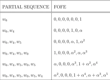
where the constantαis called forgetting factor, and it is picked between 0 and 1 ex-clusively. Obviously, the size ofzt is|V|, and it is irrelevant to the length of original sequenceT. An example is included in Table 3.1 and Table 3.2 of how to encode the sequence [w6, w4, w5, w0, w5, w4] with the vocabulary{w1, w2, w3, w4, w5, w6, w7}.

(34)

WORD 1-HOT w0 1000000 w1 0100000 w2 0010000 w3 0001000 w4 0000100 w5 0000010 w6 0000001 Table 3.1: Vocab of Size 7

PARTIAL SEQUENCE FOFE

w6 0,0,0,0,0,0,1 w6, w4 0,0,0,0,1,0, α w6, w4, w5 0,0,0,0, α,1, α2 w6, w4, w5, w0 1,0,0,0, α2, α, α3 w6, w4, w5, w0, w5 α,0,0,0, α3,1 +α2, α4 w6, w4, w5, w0, w5, w4 α2,0,0,0,1 +α4, α+α3, α5

(35)

3.4.2 Uniqueness

The word sequences can be unequivocally recovered from their FOFE representa-tions [55, 56]. The uniqueness of FOFE representation is theoretically guaranteed by the following lemma and theorems:

Lemma 1. If the forgetting factor α satisfies 0< α≤0.5, there exists exactly one element in the vector s.t. its value is no less than 1, and that element correspond to the last symbol in the sequence.

Proof. The symbol at position t is raised to αT−t, where t ∈ {_Z|1 ≤ x ≤ n}. For any symbol w in the sequence s.t. w6=wT, its value must follow

value(w)≤

T−1 X

n=1

αn<1

Theorem 2. For 0 < α ≤ 0.5, FOFE is unique for any countable vocabulary V and any finite value T.

Proof. Assume that there are two different sequences S1 = [w11, w12, ..., wT11] and S2 = [w21, w22, ..., wT22]. Denote the encoding at each time step ase1t1 and e2t2 respec-tively, where 1 ≤ t1 ≤ T1 and 1 ≤ t2 ≤ T2. To prove it by contradiction, we further assume that e1

(36)

Case 1 T1 =T2. By Lemma 1, w_T1₁ = w2_T₂. By definition, e1_T₁ = α ×e1_T₁₋₁ + oneHot(w1

T1). Because both multiplication and addition are bijective,e1T1−1 = (e1

T1−oneHot(wT11))/α, and thuse1T1−1 =e2T2−1. By induction, both sequences share the same word at the same position, which contradicts our assumption. Case 2 T1> T2. Applying the induction in Case 1, the last T2 symbols of S1 are identical to S2, and the first T2−T1 symbols of S1 has an encoding of e1_T₁₋_T₂ = e2_T₂₋_T₂ = 0. However, the first T2−T1 symbols of S1 is a non-empty sequence whose encoding cannot be0, which is a contradiction. Case 3 T1< T2. By symmetry, it leads to the same contradiction as in Case 2.

Theorem 3. For 0.5 < α < 1, given any finite value T and any countable vocab-ulary V, FOFE is unique almost everywhere, except only a finite set of countable choices of α.

Proof. Ambiguity happens when at least one symbol whose value can be composed by two disjoint sets of αt−1_{, where} _t _{∈ {}

Z|1≤t≤n}. The choice of αmust satisfy at least one of the follow polynomial equations in order to bring up ambiguity:

T

X

t=1

ξt·αt−1 = 0. (3.2)

The positive terms in Eq 3.2 represent one possible way of composition while the negative terms represent the other. Each equation is of order T, which implies at

(37)

most T −1 real roots for α. There are at most 3T equations in the same form as Eq 3.2. Therefore, it totals no more than (T −1)·3T _{choices of} _α _{that lead to}

ambiguity. 3

Though in theory uniqueness is not guaranteed when α is chosen from 0.5 to 1, in practice the chance of hitting such scenarios is extremely slim, almost impossi-ble due to quantization errors in the system. Furthermore, in natural languages, normally a word does not appear repeatedly within a near context. Simply put, FOFE is capable of uniquely encoding any sequence of arbitrary length, serving as a fixed-size but theoretically lossless representation for any sequence.

3_{The actual possible number of equations is less than 3}T _{because some of them overlap after}

simplification. The actual possible number of α is much smaller. Since one symbol’s value composition affect other symbol’s, this proof does not give a tight upper bound.

(38)

4 FOFE in Language Modeling

4.1 FOFE Language Model

The architecture of a FOFE-based neural network language model (FOFE-FFNN-LM) is shown in Figure 4.1. It is similar to regular bigram FFNN-LMs except that it feeds a FOFE into neural network LM at each time. Moreover, the FOFE can be easily scaled to higher orders like n-gram NNLMs. For example, Figure 4.2 is an illustration of a second order FOFE-FFNN-LM.

FOFE is a simple recursive encoding method but a direct sequential implemen-tation may not be efficient for the parallel compuimplemen-tation platform like GPUs. In this section, we will show that the FOFE computation can be efficiently implemented as sentence-by-sentence matrix multiplications, which are suitable for the mini-batch based SGD method running on GPUs.

Given a sentence, S = {w1, w2,· · · , wT}, where each word is represented by a

(39)

(40)

(41)

be computed based on the following matrix multiplication: S=                   1 α 1 α2 α 1 .. . . .. 1 αT−1 · · · α 1                                     e1 e2 e3 .. . eT                   =MV (4.1)

whereV is a matrix arranging all 1-of-K codes of the words in the sentence row by row, andMis aT-th order lower triangular matrix. Each row vector ofSrepresents a FOFE code of the partial sequence up to each position in the sentence.

This matrix formulation can be easily extended to a mini-batch consisting of several sentences. Assume that a mini-batch is composed of N sequences, L = {S1 S2· · ·SN}, we can compute the FOFE codes for all sentences in the mini-batch

as follows: ¯ S =              M1 M2 . .. MN                           V1 V2 .. . VN              =M ¯¯V. (4.2)

When feeding the FOFE codes to FFNN as shown in Figure 4.1, we can compute all the histories inS projected by word embedding as follow:

(42)

whereUdenotes the word embedding matrix that projects the word indices onto a continuous low-dimensional continuous space. As above,VUcan be done efficiently by looking up the embedding matrix. Therefore, for the computational efficiency purpose, we may apply FOFE to the word embedding vectors instead of the orig-inal high-dimensional one-hot vectors. In the backward pass, we can calculate the gradients with the standard BP algorithm rather than BPTT. As a result, FOFE-FFNN-LMs are the same as the standard FOFE-FFNN-LMs in terms of computational complexity in training, which is much more efficient than RNN-LMs.

4.2 Experiment Results

In order to evaluate the performance of FOFE-FFNN-LM, we have selected 3 pop-ular data sets, namely Penn TreeBank, Large Text Compression Benchmark and Google Billion Word. Each line in these corpora is a single sentence, so history does not cross sentence boundary.

We will compared the proposed model with traditional back-off n-gram LMs and the state-of-ther-art performance obtained by NNLMs. We apply the following setting by default:

• End-of-sentence symbol</s>is appended to the end of each sentence, and it is included during training and evaluation. Begin-of-sentence symbol<s> is padded to the input when history is shorter than the order of the FFNN-LM.

(43)

• When NNLM is involved, model parameters are randomly initialized by a uni-form distribution between−q 6

f anIn+f anOut and

q 6

f anIn+f anOut, wheref anIn

and f anOutare the input and the output dimensions respectively [15]. • The learning rate lr is frozen until the first non-improving epoch e. lr is

halved from the eth epoch on. We use the best learning rate chosen from {0.512,0.256,0.128,0.064,0.032} by validation set.

4.2.1 Penn TreeBank

ThePenn TreeBank(PTB) protion of the WSJ corpus has been used extensively

in LM community. In our experiment, we follow the same training/validation/test split as in other researches [40]. PTB is a small corpus. There are 930k, 74k, 82k words in training, validation and test respectively. The vocabulary is restricted to the 10k most frequent words. The rest are mapped to a special token <unk>.

PTB is relatively small. Overfitting is very likely if the model is not carefully regularized. We train using momentum [45] of 0.9 and weight decay (L2 penalty) of 0.0004. We found that the additional time and space consumption from momentum and weight decay are negligible because of PTB’s size. It also turns out that the same level of performance is not reachable with plain SGD.

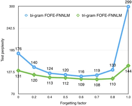
In table 4.3, we study how the forgetting factorαaffects performance. Through out this set of experiments, hyper-parameters except forgetting factor and order are

(44)

(45)

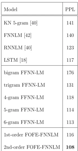
Model PPL KN 5-gram [40] 141 FNNLM [42] 140 RNNLM [40] 123 LSTM [18] 117 bigram FFNN-LM 176 trigram FFNN-LM 131 4-gram FFNN-LM 118 5-gram FFNN-LM 114 6-gram FFNN-LM 113 1st-order FOFE-FNNLM 116 2nd-order FOFE-FNNLM 108 Table 4.1: PPL on PTB for various LMs.

(46)

frozen, i.e. all experiments are with 100-dimension word embedding and 2 hidden layers of 400 nodes. We have examineα ∈ {0,0.2,0.3,0.4,0.5,0.6,0.7,0.8,1}. When α= 0, it is equivalent to bigram-FFNN-LM. We observed that whenαlies between 0.5 and 0.7, FOFE-FFNN-LM yields best performance. Therefore, we choseα = 0.7 for experiments afterwards.

We have built several baseline n-gram FFNN-LMs. Meanwhile, we have com-pared our results with known solutions in the literature. In Table 4.1, we have summarized the PPL on the PTB test set for various models. The proposed FOFE-FNNLMs significantly outperform the baseline FFNN-LMs with the same architec-ture. Moreover, the FOFE-FNNLMs even overtake a well-trained RNNLM (400 hidden units) in [40] and an LSTM in [18], which indicates that FOFE-FFNN-LMs can effectively model the long-term dependency in language without using any recurrent feedback. At last, the 2nd-order FOFE-FFNN-LM improves further, yielding the PPL of 108 on PTB. It also outperforms all higher-order FFNN-LM counterparts (4-gram, 5-gram and 6-gram), which are bigger in terms of parameter number. To our best knowledge, this is one of the best reported results on PTB without dropout [50] and model combination.

(47)

Model Architecture Test PPL KN 3-gram - 156 KN 5-gram - 132 [1*200]-400-400-80k 241 [2*200]-400-400-80k 155 FFNN-LM [2*200]-600-600-80k 150 [3*200]-400-400-80k 131 [4*200]-400-400-80k 125 RNN-LM [1*600]-600-80k 112 [1*200]-400-400-80k 120 FOFE [1*200]-600-600-80k 115 FFNN-LM [2*200]-400-400-80k 112 [2*200]-600-600-80k 107

Table 4.2: PPL on LTCB for various LMs. [M*N] denotes the sizes of the input context window and projection layer.

(48)

4.2.2 Large Text Compression Benchmark

We have further examined the modeling power of FOFE-FFNN-LMs on a larger text corpus, i.e. Large Text Compression Benchmark (LTCB) [36], which

contains the first 109 _{bytes of the English version of Wikipedia dumped in March} 3, 2006. The corpus is converted to lowercase. The most frequent 80k are kept and the rest are similarly mapped to<unk>. We have trained several baseline systems: • two n-gram LMs (3-gram and 5-gram) using the modified Kneser-Ney

smooth-ing without count cutoffs,

• several traditional FFNN-LMs with different model sizes and input context windows (bigram, trigram, 4-gram and 5-gram), and

• an RNN-LM with one hidden layer of 600 nodes using the toolkit in [39], in which we have further used a spliced sentence batch in [7] to speed up the training on GPUs.

Moreover, we have examined four FOFE-FFNN-LMs with various model sizes and input window sizes (two 1st-order FOFE models and two 2nd-order ones). For all NNLMs, we have used an output layer of the full vocabulary (80k words). In these experiments, we have used an initial learning rate of 0.1, and a bigger mini-batch of 500 for FFNN-LMMs and FOFE-FFNN-LMs, and of 256 sentences for the RNN-LMs. Since forgetting factor of 0.7 demonstrates best performance in

(49)

PTB, it is used throughout the experiments in LCTB. Overfitting seldom hap-pens when the dataset is sufficiently large. We pick SGD as our optimizer for all NNLMs without regularization. Experimental results in Table 4.2 have shown that the FOFE-FFNN-LMs significantly outperform the baseline FFNN-LMs (including some larger higher-order models) and also slightly overtake the popular RNN-LMs, yielding the best result (perplexity of 107) on the test set.

4.2.3 Google 1 Billion Benchmark

The Google Billion Word dataset [6] is one of the largest benchmark for

LM with almost one billion words. Its vocabulary size is over 800k. In order to fairly compare FOFE with known solutions, we follow the same preprocessing in [6], replacing words that occur less than 3 times with<unk>, and removing duplicated sentences.

Because computing softmax over such big vocabulary in a large scale is almost impossible, we estimate it by NCE. We have trained a medium-size and a large-size FOFE-FFNN-LMs (shown in Table 4.3). The former and the latter sample 2048 and 4096 noise examples respectively. We have tried several options of the normalization constant Z. e (base of the natural logarithm) shows the fastest convergence in the first 100 mini-batches, so we stick to this value throughout all experiments.

(50)

General speaking, the rule of thumb is that the larger the model, the better per-formance. Because of a huge vocabulary size, word embedding and NCE account for 95% of the model size. However, only a tiny portion has non-zero gradients within a mini-batch. Optimizers such as momentum and Adam [12] significantly increase time complexity and space complexity in the sense that their auxiliary data struc-ture doubles or triples memory usage and renders the sparse parameter update of word embedding and NCE impossible. It in turn prevents larger model. Therefore, we pick SGD instead of other fancy optimizers. We employ a word embedding of 256 dimensions, 3 hidden layers of{2048,4096}neurons, and a compression layer of {640,720}neurons, totaling{0.73B,0.78B}parameters, which is the biggest model that fits in a GeForce GTX TITAN X (Maxwell) of 12 GB memory.

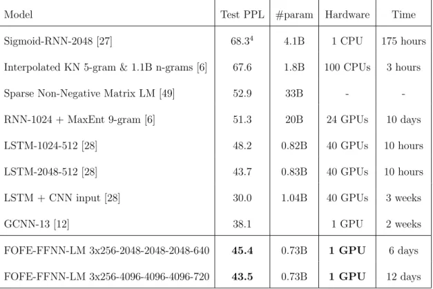
The results are presented in Table 4.3 along with the performance reported in the community. FOFE-FFNN-LM achieves similar performance with greater efficiency and less computational resources. FOFE-FFNN-LM is competitive to [28] with fewer number of parameters. However, [28] imposes demanding constraint on hardware. [12] and [28] sidestep the parameter number disaster introduced by word embedding and Softmax output by working at character level rather than word level. However, character CNN is known to be computationally expensive.

(51)

Model Test PPL #param Hardware Time

Sigmoid-RNN-2048 [27] 68.34 _4.1B _{1 CPU} _{175 hours}

Interpolated KN 5-gram & 1.1B n-grams [6] 67.6 1.8B 100 CPUs 3 hours

Sparse Non-Negative Matrix LM [49] 52.9 33B -

-RNN-1024 + MaxEnt 9-gram [6] 51.3 20B 24 GPUs 10 days

LSTM-1024-512 [28] 48.2 0.82B 40 GPUs 10 hours

LSTM-2048-512 [28] 43.7 0.83B 40 GPUs 10 hours

LSTM + CNN input [28] 30.0 1.04B 40 GPUs 3 weeks

GCNN-13 [12] 38.1 1 GPU 2 weeks

FOFE-FFNN-LM 3x256-2048-2048-2048-640 45.4 0.73B 1 GPU 6 days

FOFE-FFNN-LM 3x256-4096-4096-4096-720 43.5 0.73B 1 GPU 12 days

Table 4.3: PPL on GBW on various LMs. Some cells are blank because they are not reported.

(52)

5 FOFE in Entity Discovery

5.1 Local Detection

Our FOFE-based local detection approach for NER, calledFOFE-NERhereafter, is motivated by the way how human actually infers whether a word segment in text is an entity or mention, where the entity types of the other entities in the same sentence is not a must. Particularly, the dependency between adjacent entities is fairly weak in NER. Whether a fragment is an entity or not, and what class it may belong to, largely depend on the internal structure of the fragment itself as well as the left and right contexts in which it appears. To a large extent, the meaning and spelling of the underlying fragment are informative to distinguish named entities from the rest of the text. Contexts play a very important role in NER or MD when it involves multi-sense words/phrases or out-of-vocabulary (OOV) words.

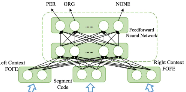
As shown in Figure 5.1, our proposed FOFE-NER method will examine all possible fragments in text (up to a certain length) one by one. For each fragment, it uses the FOFE method to fully encode the underlying fragment itself, its left

(53)

Figure 5.1: FOFE codes are fed into a FFNN. The window currently examines the fragment ofToronto Maple Leafs. The window will scan and scrutinize all fragments up to K words.

context and right context into some fixed-size representations, which are in turn fed to an FFNN to predict whether the current fragment is NOT a valid entity mention (NONE), or its correct entity type (PER, LOC, ORG and so on) if it is a valid mention. This method is appealing because the FOFE codes serves as a theoretically lossless representation of the hypothesis and its full contexts. FFNN is used as a universal approximator to map from text to the entity labels.

5.2 Feature Extraction

In this work, we use FOFE to explore both word-level and character-level features for each fragment and its contexts.

(54)

5.2.1 Word-level Features

FOFE-NER generates several word-level features for each fragment hypothesis and its left and right contexts as follows:

• Bag-of-word (BoW) of the fragment, e.g. bag-of-word vector of ‘Toronto’, ‘Maple’ and ‘Leafs’ in Figure 5.1.

• FOFE code for left context including the fragment, e.g. FOFE code of the word sequence of “... puck from space for the Toronto Maple Leafs” in Figure 5.1.

• FOFE code for left context excluding the fragment, e.g. the FOFE code of the word sequence of “... puck from space for the” in Figure 5.1..

• FOFE code for right context including the fragment, e.g. the FOFE code of the word sequence of “... against opener home ’ Leafs Maple Toronto” in Figure 5.1.

• FOFE code for right context excluding the fragment, e.g. the FOFE code of the word sequence of “... against opener home ” in Figure 5.1.

Moreover, all of the above word features are computed for both case-sensitive words in raw text as well as case-insensitive words in normalized lower-case text. These FOFE codes are projected to lower-dimension dense vectors based on two

(55)

word embedding matrices,WsandWi, for case-sensitive and case-insensitive FOFE

codes respectively. These two projection matrices are initialized by word embed-dings trained by word2vec, and fine-tuned during the learning of the neural net-works.

Due to the recursive computation of FOFE codes in eq.(3.1), all of the above FOFE codes can be jointly computed for one sentence or document in a very efficient manner.

5.2.2 Character-level Features

On top of the above word-level features, we also augment character-level features for the underlying segment hypothesis to further model its morphological structure. The aforementioned FOFE method can be easily extended to model character-level feature in NLP. Any word, phrase or fragment can be viewed as a sequence of characters. In this way, based on a pre-defined set of all possible characters, we may apply the same FOFE method to encode the sequence of characters. This always leads to a fixed-size representation, irrelevant to the number of characters in question. For the example in Figure 5.1, the current fragment, Toronto Maple Leafs, is considered as a sequence of case-sensitive characters, i.e. “{‘T’, ‘o’, ..., ‘f’ , ‘s’ }”, we then add the following character-level features for this fragment:

(56)

That is the FOFE code of the sequence, [‘T’, ‘o’, ..., ‘f ’ , ‘s’ ].

• Right-to-left FOFE code of the character sequence of the underlying fragment. That is the FOFE code of the sequence, [‘s’ , ‘f ’ , ..., ‘o’, ‘T’ ].

These case-sensitive character FOFE codes are also projected by another charac-ter embedding matrix, which is randomly initialized and fine-tuned during model training.

5.3 Training and Decoding Algorithm

Obviously, the above FOFE-NER model will take each sentence of words, S =

[w1, w2, w3, ..., wm], as input, and examine all continuous sub-sequences [wi, wi+1, wi+2, ..., wj]

up ton words inS for possible entity types. All sub-sequences longer thannwords are considered as non-entities in this work.

When we train the model, based on the entity labels of all sentences in the training set, we will generate many sentence fragments up to n words. These fragments fall into three categories:

• Exact-match with an entity label, e.g., the fragment “Toronto Maple Leafs” in the previous example.

(57)

• Disjoint with all entity label, e.g. “from space for”.

For all exact-matched fragments, we generate the corresponding outputs based on the types of the matched entities in the training set. For both partial-overlap and disjoint fragments, we introduce a new output label,NONE, to indicate that these fragments are not a valid entity. Therefore, the output nodes in the neural networks contain all entity types plus a rejection option denoted as NONE.

During training, we implement a producer-consumer software design such that a thread fetches training examples, computes all FOFE codes and packs them as a mini-batch while the other thread feeds the mini-batches to neural networks and adjusts the model parameters and all projection matrices. Since “partial-overlap” and “disjoint” significantly outnumber “exact-match”, they are down-sampled so as to balance the data set. The training procedure is illustrated in Algorithm 1.

During inference, all fragments not longer than n words are all fed to FOFE-NER to compute their scores over all entity types. In practice, these fragments can be packed as one mini-batch so that we can compute them in parallel on GPUs. As the NER result, the FOFE-NERmodel will return a subset of fragments only if: i) they are recognized as a valid entity type (not NONE); AND ii) their NN scores exceed a global pruning threshold.

Occasionally, some partially-overlapped or nested fragments may occur in the above pruned prediction results. We can use one of the following simple

(58)

post-Algorithm 1 FOFE-NER TRAINING algorithm

1: procedure train(S, o, d, n) . S: labeled sentence set . n: maximum ner length . o: overlap sample rate . d: disjoint sample rate

2: data← {} 3: for [w1, w2, ..., wl] in S do 4: for i←1...l do 5: for j ←i, min(l, i+n−1) do 6: f ←f eature([wi, ..., wj]) 7: t←label([wi, ..., wj])

8: if overlap([wi, ..., wj]) and rand(0,1)> o then

9: continue

10: end if

11: if disjoint([wi, ..., wj]) and rand(0,1)> d then

12: continue

(59)

14: data←data∪ {(f, t)}

15: end for

16: end for

17: end for

18: for minibatch indata do

19: DN Nf of e.train(minibatch)

20: end for

21: end procedure

processing methods to remove overlappings from the final results:

1. highest-first: We check every word in a sentence. If it is contained by more than one fragment in the pruned results, we only keep the one with the maximum NN score and discard the rest. It is listed in Algorithm 4.

2. longest-first: We check every word in a sentence. If it is contained by more than one fragment in the pruned results, we only keep the longest fragment and discard the rest. It is listed in Algorithm 5.

Either of these strategies leads to a collection of nested, overlapping, non-NONE entity labels.

In some tasks, it may require to label all nested entities. This has imposed a big challenge to the sequence labeling methods. However, the above post-processing

(60)

can be slightly modified to generate nested entities’ labels. In this case, we first run either highest-first or longest-first to generate the first round result. For every entity survived in this round, we will recursively run either highest-first or longest-first on all entities in the original set, which are completely contained by it. The decoding precedure is detailed in Algorithm 2 and Algorithm 3. This will generate more prediction results. This process may continue to allow any levels of nesting. For example, for a sentence of “w1 w2 w3 w4 w5”, if the model first generates the prediction results after the global pruning, as [“w2w3”, PER, 0.7], [“w3w4”, LOC, 0.8], [“w1w2w3w4”, ORG, 0.9], if we choose to runhighest-first, it will generate the first entity label as [“w1w2w3w4”, ORG, 0.9]. Secondly, we will run highest-first on the two fragments that are completely contained by the first one, i.e., [“w2w3”, PER, 0.7], [“w3w4”, LOC, 0.8], then we will generate the second nested entity label as [“w3w4”, LOC, 0.8]. Fortunately, in any real NER and MD tasks, it is pretty rare to have overlapped predictions in the NN outputs. Therefore, the extra expense to run this recursive post-processing method is minimal.

5.4 Second-Pass Augmentation

As we know, CRF brings marginal performance gain to all taggers (but not limited to NER) because of the dependencies (though fairly weak) between entity types. We may easily add this level of information to our model by introducing another

(61)

Algorithm 2 ELIMINATE OVERLAP algorithm

1: procedure del recur(scores, [algo1, algo2, ..., algox], [t1, t2, ..., tx])

. x: desired level of nested mention

.[t1, t2, ..., tx]: threshold at each nested level . scores: (i, j, labeli,j, scorei,j) tuples

. n: maximum ner length

2: assert algo1 ∈ { highest–f irst, longest–f irst}

3: candidates← {(i, j, labeli,j, scorei,j)|

(i, j, labeli,j, scorei,j)∈scores and scorei,j ≥t1}

4: result←algo1(candidates)

5: nested← {}

6: for (i, j, labeli,j, scorei,j)∈result do

7: sub← {(x, y, labelx,y, scorex,y)|

(x, y, labelx,y, scorex,y)∈scores and (i≤x≤y < j or i < x≤y ≤j)}

8: nested ←nested ∪ DEL RECUR(sub,[algo2, algo3, ..., algox],[t2, t3, ..., tx])

9: end for

10: return result∪nested

(62)

Algorithm 3 FOFE-NER DECODING algorithm

1: procedure _decode([w1, w2, ..., wl],

[algo1, algo2, ..., algox], [t1, t2, ..., tx],n)

.[w1, w2, ..., wl]: a sentence

. n: maximum ner length

. x: level of desired nested mention to detect .[t1, t2, ..., tx]: threshold at each nested level

. [algo1, algo2, ..., algox]: algorithms used to eliminate overlapping of each

nested level

2: r← {} .r: temporary results

3: for i←1...l do

4: for j ←i...min(l, i+n−1)do

5: f ←f eature([wi, ..., wj])

6: labeli,j, scorei,j ←DN Nf of e.eval(f)

7: if labeli,j 6=N ON E then

8: r←r∪ {(i, j, labeli,j, scorei,j)}

9: end if

10: end for

11: end for

(63)

Algorithm 4 HIGHEST-FIRST DECODING algorithm

1: function highest1st(scores, l) . scores: (i, j, labeli,j, scorei,j) tuples

. l: sentence length

2: for k ←1...l do

3: removed← {}

4: candidates ← {(i, j, labeli,j, scorei,j)|

(i, j, labeli,j, scorei,j)∈scores and i≤k ≤j}

5: candidates ←sortByScore(candidates)

6: if |candidates|>0then

7: candidates←removeHighestScore(candidates)

8: end if

9: removed←removed∪candidates

10: end for

11: estimate←sortByStartIdx(scores−removed)

12: estimate←mergeAdjacientOf SameT ype(estimate)

13: return estimate

(64)

Algorithm 5 LONGEST-FIRST DECODING algorithm

1: function longest1st(scores, l) . scores: (i, j, labeli,j, scorei,j) tuples

. l: sentence length

2: best←createEmptyList()

3: candidate←createHashedM ap()

4: for (i, j, labeli,j, scorei,j)∈scores do candidate[(i, j)]←labeli,j

5: end for 6: for i←1...l do 7: cur ←createEmptyList() 8: if (1, i)∈candidate then 9: cur.insert((1, i)) 10: best.insert((1, cur)) 11: else 12: best.insert((0, cur)) 13: end if 14: for j ←1...ido 15: newLen←best[j][0] +i−j+ 1

16: if (j, i)∈candidate and newLen > head(lastOf(best)) then

(65)

18: best.insert((newLen,(j + 1, i+ 1))

19: end if

20: end for

21: last, secondLast←lastOf(best), secondLastOf(best)

22: if i >1 and head(last)> head(secondLast)then

23: best.pop()

24: best.insert(secondLast)

25: end if

26: end for

27: estimate←mergeAdjacientOf SameT ype(estimate)

28: return estimate

(66)

pass of FOFE-NER. We call it 2nd-pass FOFE-NER.

In 2nd-pass FOFE-NER, another set of model is trained on outputs from the first-passFOFE-NER, including all predicted entities. For example, given a sen-tence

S = [w1, w2, ...wi, ...wj, ...wn]

and an underlying word segment [wi, ..., wj] in the second pass, every predicted

entity outside this segment is substituted by its entity type predicted from the first pass. For example, in the first pass, a sentence like “Google has also recruited Fei-Fei Li, director of the AI lab at Stanford University.” is predicted as: “<ORG> has also recruited Fei-Fei Li, director of the AI lab at <ORG>.” In 2nd-pass FOFE-NER, when examining the segment “Fei-Fei Li”, the predicted entity types <ORG>are used to replace the actual named entities. The 2nd-pass FOFE-NER model is trained on the outputs of the first pass, where all detected entities are replaced by their predicted types as above. The training process is depicted in Figure 5.2.

During inference, the results returned by the 1st-pass model are substituted in the same way. The scores for each hypothesis from 1st-pass model and 2nd-pass model are linear interpolated and then decoded by eitherhighest-firstorlongest-first to generate the final results of 2nd-pass FOFE-NER.

(67)

en-Figure 5.2: Illustration of the 2nd-pass Augmentation

tities while filtering out unwanted constructs and sparse combinations. On the other hand, it enables longer context expansion, since FOFE memorizes contextual information in an unselective decaying fashion.

5.5 Experiment Results

In this section, we evaluate the effectiveness of our proposed methods on several popular NER and MD tasks, including CoNLL 2003 NER task and TAC-KBP2015

(68)

and TAC-KBP2016 Tri-lingual Entity Discovery and Linking (EDL) tasks. 5

5.5.1 CoNLL 2003 NER task

The CoNLL2003 dataset [47] consists of newswire from the Reuters RCV1 corpus tagged with four types of non-nested named entities: location (LOC), organiza-tion (ORG), person (PER), and miscellaneous (MISC). Table 5.2 shows the data distribution of CoNLL2003 dataset.

The top 100,000 words, are kept as vocabulary, including punctuations. For the case-sensitive embedding, an OOV is mapped to<unk>; if it contains no upper-case letter and<UNK>; otherwise. We perform grid search on several hyper-parameters using a held-out dev set. Here we summarize the set of hyper-parameters used in our experiments:

• Learning rate: initially set to 0.128 and is multiplied by a decay factor each epoch so that it reaches 1/16 of the initial value at the end of the training; • Network structure: 3 fully-connected layers of 512 nodes with ReLU

activa-tion, randomly initialized based on a uniform distribution between−q 6

Ni+No

and q_N 6

i+No [15];

• Character embeddings: 64 dimensions, randomly initialized between -1 and 1. 5_{We have made our codes available at}

https://github.com/xmb-cipher/fofe-nerfor read-ers to reproduce the results in this paper.

(69)

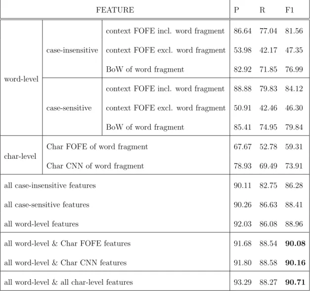
FEATURE P R F1

word-level

case-insensitive

context FOFE incl. word fragment 86.64 77.04 81.56 context FOFE excl. word fragment 53.98 42.17 47.35 BoW of word fragment 82.92 71.85 76.99

case-sensitive

context FOFE incl. word fragment 88.88 79.83 84.12 context FOFE excl. word fragment 50.91 42.46 46.30 BoW of word fragment 85.41 74.95 79.84

char-level

Char FOFE of word fragment 67.67 52.78 59.31

Char CNN of word fragment 78.93 69.49 73.91

all case-insensitive features 90.11 82.75 86.28

all case-sensitive features 90.26 86.63 88.41

all word-level features 92.03 86.08 88.96

all word-level & Char FOFE features 91.68 88.54 90.08

all word-level & Char CNN features 91.80 88.58 90.16

all word-level & all char-level features 93.29 88.27 90.71

(70)

Articles Sentences Tokens LOC MISC ORG PER

train 946 14,987 203,621 7,140 3,438 6,321 6,600

dev 216 3,466 51,362 1,837 922 1,341 1,842

test 231 3,684 46,435 1,668 702 1,661 1,617

Table 5.2: Data distribution of CoNLL2003 • mini-batch: 512;

• Dropout Rate: initially set to 0.4, slowly decreased during training until it reaches 0.1 at the end.

• Number of Epochs: 128;

• Word Embedding: case-sensitive and case-insensitive word embeddings of 256 dimensions, trained from Reuters RCV1;

• We stick to the official data train-dev-test partition. • Forgetting Factor: α= 0.5. 6

• Character CNN: The same method in Section 2.2.2 is applied. 8 sets of kernels are used, whose heights range from 2 to 9. Each set of kernels of depth 16. 6_{The choice of the forgetting factor}_α_{is empirical. We’ve evaluated}_α_{= 0}_.₅_,₀_.₆_,₀_.₇_,₀_._{8 on a}

development set in some early experiments. It turns out that α= 0.5 is the best. As a result,

(71)

The character embedding is not shared with FOFE character embedding but initialized in the same way.

We have investigated the performance of our method on the CoNLL-2003 dataset by using different combinations of the FOFE features (both word-level and character-level). The detailed comparison results are shown in Table 5.1. In Table 5.3, we have compared our best performance with some top-performing neural network sys-tems on this task. As we can see from Table 5.3, our system (highest-first decoding) yields very strong performance (90.85 inF1 score) in this task, outperforming most of neural network models reported on this dataset. More importantly, we have not used any hand-crafted features in our systems, and all features (either word or char level) are automatically derived from the data. Highest-first and longest-first per-form similarly. In [8]7_{, a slightly better performance (91.62 in}_F

1 score) is reported but a customized gazetteer is used in theirs.

5.5.2 KBP2015 EDL Task

Given a document collection in three languages (English, Chinese and Spanish), the KBP2015 tri-lingual EDL task [26] requires to automatically identify entities (including nested entities) from a source collection of textual documents in 7_{In their work, they have used a combination of training-set and dev-set to train the model,}

(72)

algorithm word char gaz cap pos F1 CNN-BLSTM-CRF [9] ₃ ₇ ₃ ₃ ₇ 89.59 BLSTM-CRF [24] ₃ ₃ ₃ ₃ ₃ 90.10 BLSTM-CRF [46] ₃ ₇ ₃ ₃ ₃ 89.28 BLSTM-CRF, char-CNN [8] ₃ ₃ ₃ ₇ ₇ 91.62 Stack-LSTM-CRF, char-LSTM [32] ₃ ₃ ₇ ₇ ₇ 90.94 FOFE-NER 3 3 7 7 7 90.71 FOFE-NER + dev-set 90.92 FOFE-NER + 2nd-pass 90.85

FOFE-NER + dev-set + 2nd-pass 91.17

Table 5.3: Performance (F1 score) comparison among various neural models re-ported on the CoNLL2003 dataset, and the different features used in these meth-ods.

(73)

English Chinese Spanish ALL

Train 168 147 129 444

Eval 167 167 166 500

Table 5.4: Number of Documents in KBP2015

multiple languages as in Table 5.4, and classify them into one of the following pre-defined five types: Person (PER), Geo-political Entity (GPE), Organization (ORG), Location (LOC) and Facility (FAC). The corpus consists of news articles and discussion forum posts published in recent years, related but non-parallel across languages.

Three models are trained and evaluated independently. Unless explicitly listed, hyperparameters follow those used for CoNLL2003 as described in section 5.5.1 and 2nd-pass model is not used. Three sets of word embeddings of 128 dimensions are derived from English Gigaword [44], Chinese Gigaword [16] and Spanish Gigaword [38] respectively. Some language-specific modifications are made:

• Chinese: Because Chinese segmentation is not reliable, we label Chinese at character level. The analogous roles of case-sensitive word-embedding and case-sensitive embedding are played by character embedding and word-embedding in which the character appears. Neither Char FOFE features nor Char CNN features are used for Chinese.

(74)

2015 track best ours P R F1 P R F1 Trilingual 75.9 69.3 72.4 78.3 69.9 73.9 English 79.2 66.7 72.4 77.1 67.8 72.2 Chinese 79.2 74.8 76.9 79.3 71.7 75.3 Spanish 78.4 72.2 75.2 79.9 71.8 75.6

Table 5.5: Entity Discovery Performance of our method on the KBP2015 EDL eval-uation data, with comparison to the best systems in KBP2015 official evaleval-uation.

• Spanish: Character set of Spanish is a super set of that of English. When building character-level features, we use the mod function to hash each charac-ter’s UTF8 encoding into a number between 0 (inclusive) and 128 (exclusive).

As shown in Table 5.5, our FOFE-based local detection method has obtained fairly strong performance in the KBP2015 dataset. The overall trilingual entity discovery performance is slightly better than the best systems participated in the official KBP2015 evaluation, with 73.9 vs. 72.4 as measured by F1 scores. Outer and inner decodings are longest-first and highest-firstrespectively.

(75)

LANG OVERALL 2016 BEST P R F1 P R F1 ENG 0.836 0.680 0.750 0.846 0.710 0.772 CMN 0.789 0.625 0.698 0.789 0.737 0.762 SPA 0.835 0.602 0.700 0.839 0.656 0.736 ALL 0.819 0.639 0.718 0.802 0.704 0.756

Table 5.6: Official entity discovery performance of our methods on KBP2016 trilin-gual EDL track. Neither KBP2015 nor in-house data labels nominal mentions. Nominal mentions in Spanish are totally ignored since no training data is found for them.

(76)

English Chinese Spanish ALL

Eval 167 168 168 503

Table 5.7: Number of Documents in KBP2016

5.5.3 KBP2016 EDL task

In KBP2016, the trilingual EDL task is extended to detect nominal mentions of all 5 entity types for all three languages. In our experiments, for simplicity, we treat nominal mention types as some extra entity types and detect them along with named entities together with a single model.

training data P R F1

KBP2015 0.836 0.598 0.697

KBP2015 + WIKI 0.837 0.628 0.718 KBP2015 + in-house 0.836 0.680 0.750

Table 5.8: Our entity discovery official performance (English only) in KBP2016 is shown as a comparison of three models trained by different combinations of training data sets.

Fixed Size Ordinally-Forgetting Encoding and its Applications

Abstract

Acknowledgements

Table of Contents

List of Tables

List of Figures

Abbreviations

1

Introduction

1.1

Motivation

1.2

Contribution and Outline of the Thesis

2

Literature Review

2.1

Deep Learning

2.2

Vector Representation of Words

2.3

Two Fundamental Problems in NLP

3

Fixed-size Ordinally Forgetting Encoding

3.1

One-Hot Encoding

3.2

Bag of Words

3.3

Term Frequency - Inverse Document Frequency

3.4

Fixed-size Ordinally Forgetting Encoding

4

FOFE in Language Modeling

4.1

FOFE Language Model

4.2

Experiment Results

5

FOFE in Entity Discovery

5.1

Local Detection

5.2

Feature Extraction

5.3

Training and Decoding Algorithm

5.4

Second-Pass Augmentation

5.5

Experiment Results