Efficient 3D medical image segmentation

(1)

Some pages of this thesis may have been removed for copyright restrictions.

If you have discovered material in Aston Research Explorer which is unlawful e.g. breaches

copyright, (either yours or that of a third party) or any other law, including but not limited to

those relating to patent, trademark, confidentiality, data protection, obscenity, defamation,

libel, then please read our

Takedown policy

and contact the service immediately

(2)

Efficient 3D Medical

Image Segmentation.

MR BENJAMIN JOE FLETCHER

Master of Philosophy

ASTON UNIVERSITY

May 2014

Benjamin Joe Fletcher asserts his moral right to be identified as the author of this thesis.

This copy of the thesis has been supplied on condition that anyone who consults it is understood to recognise that its copyright rests with its author and that no quotation from the thesis and no information derived from it may be published

(3)

Aston University

Efficient 3D Medical Image Segmentation

Mr Benjamin Joe Fletcher, Master of Philosophy, 2014

Synopsis

3D Medical imaging techniques have become extremely important tools in patient diagnosis. However, they produce large amounts of data that is difficult to interpret, and can currently only be analysed by highly trained people.

Datasets are large – the female Visible Human dataset is around 40 Gb in size. Processing any dataset of this size will obviously be computationally demanding.

Currently segmentation of images is a predominantly manual process. Tools that are available allow segmentation to be done on a slice-by-slice basis, often using a flood-fill or region growing approach based on colour or texture space.

This report outlines research into an automated texture based segmentation technique. The research compared the effectiveness of using simple and energy efficient DCT (Discrete Cosine Transform) and Haar transforms (in both 2D and 3D forms) as a description of texture at each location within an image. This description was initially used as a vector in feature space, allowing segmentation to be carried out using a Gaussian Mixture Model and some post processing techniques. The transforms were then extended to make them independent of variations in intensity, a common issue in medical imaging. However, although now robust to intensity variations, the results were not of sufficient quality to be useful in a real application.

To improve the quality of results, a model based approach based on an AAM (Active Appearance Model) was considered. A traditional AAM uses an intensity based appearance model, which while less computationally demanding than a more complex texture based appearance model, can give poor results when subjected to intensity variations. When complex texture descriptions are used to create the appearance model results are much improved, but this is at the expense of run time, which can make the techniques less practical.

A novel combination of mDCT (modified DCT, which is intensity invariant) and an AAM was implemented and tested. When presented with 3D volumes which had been subjected to intensity variations this was seen to generate much better results than a traditional AAM, while maintaining a practical run time.

Using this approach the time taken to carry out segmentations was less than 10 minutes (when run in Matlab on a typical datacentre based Linux machine). This showed the process to be practical in terms of quality of results, run time and energy efficiency.

Keywords: Active Appearance Model, Discrete Cosine Transform, Haar Transform, Intensity Invariant

(4)

(5)

Dedication

This thesis is dedicated to Lara, who I had not met when I started working on it, and yet only through our meeting was I able to complete it.

And to Oscar, who makes sure every day is different to the last.

Also to my family who have provided endless encouragement and support.

To Max, Henry, Joe and Charlie, just because.

(6)

(7)

Acknowledgements

I would like to acknowledge my supervisor I.T.Nabney for his guidance and support.

I would also like to acknowledge the Visible Human Project for providing access to their datasets.

Much of the experimental work was based on code made available by D.Kroon [20].

(8)

(9)

List of Tables

Table 1: Fitting Time of AAM in seconds when using appearance model based

on Intensity and GLBP [19]. ... 66

Table 2: Details of the Visible Human Project data. ... 72

Table 3: Details about the upper arm bone dataset. ... 80

Table 4: Example slices and segmentations from the upper arm bone dataset. 80 Table 5: Details about the upper left leg bone dataset. ... 81

Table 6: Example slices and segmentations from the upper left leg bone dataset. ... 81

Table 7: Details about the upper right leg bone dataset. ... 82

Table 8: Example slices and segmentations from the upper right leg bone dataset. ... 82

Table 9. results from a groups of experiments based on a block size of 4x4 pixels, and a 2D DCT transform. ... 85

Table 10. The Mean, variance and Standard deviation for the data presented in table 9. ... 85

Table 11: thresholds used in low pass filters. ... 114

Table 12: Comparison of results between different transforms. ... 115

Table 13: Comparison of sampling size against transform ... 119

Table 14: Comparison of sampling size against feature space dimensions and resulting run time. ... 120

Table 15: Summary of number of operations required to carry out different sized transforms. ... 125

Table 16: Summary of results using the Haar Short transform (2D and 3D). .. 126

Table 17: Observed run times from various Haar Short transforms. ... 127

Table 18: Observations when different filters are used... 130

Table 19: The results of using a 2D low pass filter against using both a 2D and 3D low pass filter. ... 136

Table 20: Results for DCT LONG 2D Transform over a 40 point variation in intensity, when the process uses the DC coefficient from the DCT transform. 147 Table 21: Results for DCT LONG 2D Transform over a 40 point variation in intensity, when the process does not use the DC coefficient from the DCT transform. ... 147

(13)

Table 22: Results for DCT LONG 3D Transform over a 40 point variation in intensity, when the process uses the DC coefficient from the DCT transform. 149 Table 23: Results for DCT LONG 3D Transform over a 40 point variation in intensity, when the process does not use the DC coefficient from the DCT

transform. ... 150

Table 24: Results for HAAR LONG 2D Transform over a 40 point variation in intensity, when the process uses the DC coefficient from the HAAR transform. ... 151

Table 25: Results for HAAR LONG 2D Transform over a 40 point variation in intensity, when the process does not use the DC coefficient from the HAAR transform. ... 152

Table 26: Results for HAAR LONG 3D Transform over a 40 point variation in intensity, when the process uses the DC coefficient from the HAAR transform. ... 153

Table 27: Results for HAAR LONG 3D Transform over a 40 point variation in intensity, when the process does not use the DC coefficient from the HAAR transform. ... 154

Table 28. Post processing that was carried out during initial segmentations of the more complex dataset. ... 170

Table 29: Results on more complex segmentation. ... 171

Table 30: outline of post processing used in the updated segmentation. ... 175

Table 31: Results seen when using an initial region growing process. ... 175

Table 32: outline of post processing used in segmentation. ... 178

Table 33: Post processing steps that were carried out to investigate the use of different 2D transforms. ... 182

Table 34: Comparison of results using different 2D transforms. ... 183

Table 35: summary of post processing steps used in the generation of the final results. ... 183

Table 36: Final results for the complex segmentation set, using post processing as described in table 35. ... 184

Table 37: Summary of datasets that were created. ... 188

Table 38: Summary of techniques used to distort image data. ... 189

Table 39: Summary of test datasets that were created. ... 189

(14)

Table 41: description of test sets used to evaluate effectiveness of a 2D AAM. ... 200 Table 42: Results when using intensity-based appearance model, and

undistorted test set. ... 201 Table 43: Results when using intensity-based appearance model, and

constrained randomly distorted test set. ... 202 Table 44: Results when using mDCT-based appearance model, and undistorted test set. ... 202 Table 46: Summary of datasets used to evaluate the effectiveness of a 3D AAM approach with various appearance models. ... 211 Table 47: Summary of results using a 3D AAM to segment previously unseen eyes at various scales ranging from 60% to 100%. ... 213 Table 48: Summary of results using a 3D AAM to segment previously unseen eyes at a scale of 100%. ... 215 Table 49: Results when using an intensity based appearance model and a single colour channel training and test dataset (scale 60% - 80%). ... 230 Table 50: Results when using an intensity based appearance model and a single colour channel training and test dataset (scale 90% - 100%). ... 232 Table 51: Results when using a 2x2 mDCT based appearance model and a single colour channel training and test dataset (scale 60% - 80%). ... 234 Table 52: Results when using a 2x2 mDCT based appearance model and a single colour channel training and test dataset (scale 90% - 100%). ... 236 Table 53: Results when using a 2x2x2 mDCT based appearance model and a single colour channel training and test dataset (scale 60% - 80%). ... 238 Table 54: Results when using a 2x2x2 mDCT based appearance model and a single colour channel training and test dataset (scale 90% - 100%). ... 240 Table 55: Results when using an intensity based appearance model and a three colour channel training and test dataset (scale 60% - 80%). ... 242 Table 56: Results when using an intensity based appearance model and a three colour channel training and test dataset (scale 90% - 100%). ... 244 Table 57: Results when using a 2x2 mDCT based appearance model and a three colour channel training and test dataset (scale 60% - 80%). ... 246 Table 58: Results when using a 2x2 mDCT based appearance model and a three colour channel training and test dataset (scale 90% - 100%). ... 248

(15)

Table 59: Results when using a 2x2x2 mDCT based appearance model and a three colour channel training and test dataset (scale 60% - 80%). ... 250 Table 60: Results when using a 2x2x2 mDCT based appearance model and a three colour channel training and test dataset (scale 90% - 100%). ... 252

(16)

(17)

List of Figures

Figure 1: Images from the Visible Human Project. ... 23

Figure 2: Diagram of a simple CT scanner. ... 30

Figure 3. An example of aliasing occurring even though the Nyquist criteria has been observed. Input data (top left) sampled by aligned sampling windows (top right). Input data (bottom left) sampled by non-aligned sampling windows (bottom right). Data being sampled is shown in blue. Result of sampling is shown in green. ... 33

Figure 4: Illustration of the Partial Volume Effect. On the left, the real object (with a grid representing the sampling resolution). On the right, the resulting sampled image. ... 34

Figure 5: Photon pairs as observed by a PET scanner. ... 37

Figure 6: Physical layout of an MRI scanner. ... 39

Figure 7: A typical region growing algorithm (in pseudo code). ... 43

Figure 8: basis functions used by a DCT, being calculated over a data series of 8 samples. ... 44

Figure 9: basis functions used by a DCT, being calculated over a 2-dimensional data series of 8x8 samples. ... 47

Figure 10: Example showing the shape of two Gaussian distributions, which have different values for mean and standard deviation. ... 49

Figure 11: A probability distribution based on combining the two Gaussian distributions shown in figure 10. ... 51

Figure 12: a graphical depiction of the Haar wavelets basis functions –based on the mother function, shifted and dilated for use at various scales and locations across the input data. ... 53

Figure 13: The Haar wavelet basis functions, expressed as a series of vectors. ... 53

Figure 14: The zigzag ordering of the coefficients that is used to construct the optimal sequence for entropy encoding. ... 57

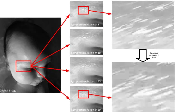
Figure 15: the effect of increasing the compression ration used when storing an image in JPEG format. ... 58

Figure 16: Example of warping using triangulation. A point in the original triangle (bottom left) is mapped to the equivalent point in the new triangle (top right). .. 60

(18)

Figure 17: Example slice from the Visible Human Project (cryosection dataset).

... 71

Figure 18: A close up of an area of 8x8 pixels taken from the centre of an image (top). The same area split into blocks (bottom left and bottom right). ... 76

Figure 19: A sample of a plot showing the results of a segmentation. ... 86

Figure 20. Original image (top left). Image with high frequency components removed, using transform D1 (top right). Image with DC coefficient removed, using transform D2 (bottom left). Image with both DC coefficients and high frequency components removed, using transform D3 (bottom right). ... 92

Figure 21: Mapping between output coefficients of a Haar transform, and the input coefficients that affect them. ... 96

Figure 22: Mapping of Haar transform coefficients to a Haar short descriptor for a specific sub-block. ... 97

Figure 23: Flow chart showing the process used to investigate the DCT and Wavelet transforms as a measure of texture in medical images. ... 100

Figure 24: phase one of search. ... 103

Figure 25: Blocks are sampled, and descriptors calculated in advance. The starting threshold is set such that 80% of the segmentation set are above the threshold (based on the manual segmentation). ... 104

Figure 26: phase 2 of search. ... 105

Figure 27: pseudo code representation of phase two of the search. ... 106

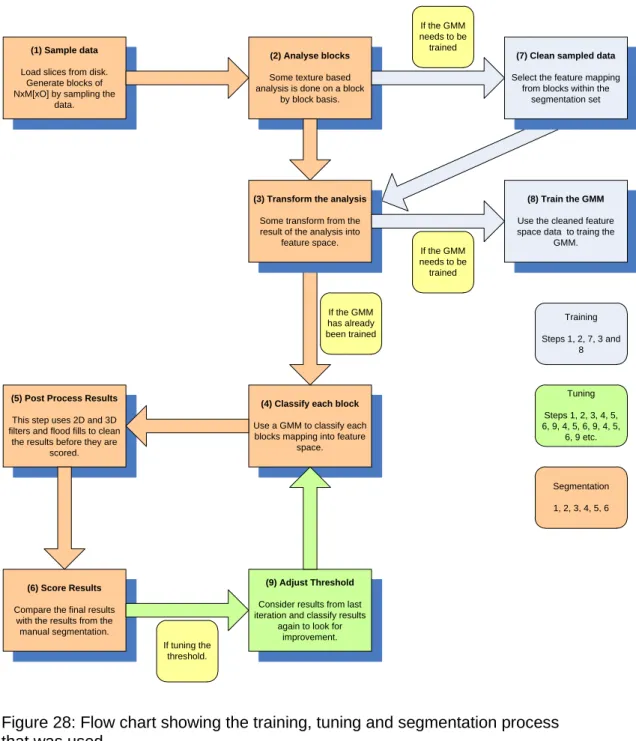
Figure 28: Flow chart showing the training, tuning and segmentation process that was used. ... 109

Figure 29: example of a week region growing process with the seed location marked. ... 111

Figure 30: Example of a strong region growing process... 112

Figure 31: Example of an asymmetric and symmetric low pass filter. ... 113

Figure 32: Results using 2D 2x2x1 DCT. ... 116

Figure 35: Results using 2D 2x2x1 Haar ... 117

Figure 36: Results using 2D 4x4x1 Haar. ... 118

Figure 37: Results using 2D 8x8x1 Haar ... 118

Figure 38: results using 3D 4x4x2 DCT. ... 121

(19)

Figure 43: Results using a 3D 8x8x2 Haar ... 123

Figure 44: Two slices processed with 2D 4x4 Haar Short transform. ... 128

Figure 45: Two slices processed with 2D 4x4 Haar short transform, with a 2D low pass filter applied to raw segmentation results, before a strong region growing process was applied. ... 132

Figure 46: Two slices processed with 2D 4x4 Haar short transform, with a 3D low pass filter applied to raw segmentation results, before a strong region growing process was applied. ... 133

Figure 47: Slice 4, when testing a combination of 2D and 3D low pass filter. . 137

Figure 51: Results when input image has had its intensity decreased by 20. . 143

Figure 52: Results when input image has had its intensity decreased by -12. 144 Figure 53: Results when input image has had its intensity decreased by 4. ... 144

Figure 54: Results when input image has had its intensity increased by 4. .... 145

Figure 55: Results when input image has had its intensity increased by 12. .. 145

Figure 57: Plot showing the comparison of results between the Intensity Variant and Intensity Invariant methods for the DCT LONG 2D transform. ... 148

Figure 58: Plot showing the comparison of results between the Intensity Variant and Intensity Invariant methods for the DCT LONG 3D transform. ... 150

Figure 59: Plot showing the comparison of results between the Intensity Variant and Intensity Invariant methods for the HAAR LONG 2D transform. ... 152

Figure 60: Plot showing the comparison of results between the Intensity Variant and Intensity Invariant methods for the HAAR LONG 3D transform. ... 155

Figure 61: Although the results are now consistent over intensity variation, there are still anomalies present. ... 156

Figure 62: Locations with any response over the threshold are included in the segmentation set. ... 157

Figure 63: Results when input image has had its intensity decreased by 20. . 158

(20)

Figure 65: Results when input image has had its intensity increased by 8. .... 159

Figure 67: Pseudo code showing operation of minimum and maximum threshold. ... 160

Figure 68: Example of segmentation where lack of a maximum threshold causes the segmentation to fail completely. ... 161

Figure 69: Example of segmentation where lack of a maximum threshold causes the segmentation to fail completely. ... 162

Figure 70: Although the previous anomaly has gone, a new anomaly has appeared. ... 163

Figure 71: Left hand image shows the raw results before a maximum threshold was used. Right hand image shows the raw results once a maximum threshold has been used. The white oval annotation on the right hand image shows the approximate location of the desired segmentation. ... 164

Figure 72: DCT Long 2D based segmentation results. ... 166

Figure 73: DCT Long 3D based segmentation results. ... 166

Figure 74: Haar Long 2D based segmentation results. ... 167

Figure 75: Haar Long 3D based segmentation results. ... 167

Figure 76: Haar Short 2D based segmentation results. ... 168

Figure 77: Haar Short 3D based segmentation results. ... 168

Figure 78: Upper Leg Bone. ... 169

Figure 79: The region between the two white ovals is roughly the outer border of a bone in the upper leg. ... 170

Figure 80: More complex segmentation, attempted using 3D Haar Long transforms, and post processing as described in table 28. ... 172

Figure 81: More complex segmentation, attempted using 3D DCT Long transforms, and post processing as described in table 28. ... 173

Figure 82: More complex segmentation, attempted using 2D Haar Long transforms, and post processing as described in table 28. ... 173

Figure 83: More complex segmentation, attempted using 2D DCT Long transforms, and post processing as described in table 28. ... 174

Figure 84: Segmentation preformed using 2D Haar Long transforms, and using post processing as outlined in table 30. ... 176

Figure 85: Segmentation preformed using 2D Haar Long transforms, and using post processing as outlined in table 30. ... 176

(21)

Figure 86: Segmentation preformed using 2D DCT Long transforms, and using

post processing as outlined in table 30. ... 177

Figure 87: Segmentation preformed using 2D DCT Long transforms, and using post processing as outlined in table 30. ... 177

Figure 88: raw results (left) and results with after a strong region growing process had been applied (right). ... 178

Figure 89: raw results (left) and results after a weak region growing process had been applied (right). ... 179

Figure 90: raw results (left) and results after a strong region growing process had been applied (right). ... 179

Figure 91: raw results (left) and results after a weak region growing process had been applied (right). ... 180

Figure 92: The initial low pass filter was responsible for over eroding the results. ... 181

Figure 93: Using a symmetric low pass filter (top) and an asymmetric low pass filter (bottom). ... 182

Figure 94: Sample of images from the Cohn-Kanade dataset. ... 186

Figure 95: Various slices used to investigate a 2D AAM ... 193

Figure 96: Manual segmentation of slices shown in figure 87 ... 194

Figure 97. The manual segmentation of two slices, with the segmenation set shown in green. The blue star marks the calculated centre point of the sementation, and the yellow stars mark the calculated boundary points which are used as landmarks... 197

Figure 98: Segmentation generated when a small level of distortion applied to the test dataset, and an intensity based AAM is used. ... 204

Figure 99: Segmentation generated when a small level of distortion applied to the test dataset, and a mDCT based AAM is used. ... 205

Figure 100: Slice 1139 when segmented using intensity based appearance model. ... 206

Figure 101: Slice 1139 when segmented using an mDCT based appearance model. ... 206

Figure 102: Undistorted slice 1137 (top left). Distorted slice 1137 (top right). Output of mDCT texture analysis of undistorted slice 1137 (bottom left). Output of mDCT texture analysis of distorted slice 1137 (bottom right). ... 207

(22)

Figure 103: A view of some of the landmarks of two adjance slices. The verticies of each triangular face are landmarks (marked with stars). ... 209 Figure 104: shows a wire frame representation of the surface model used in the 3D AAM. ... 210 Figure 105: Shows a slice through a full 3D segmentation of an eye. In this case 99% of voxels were classified correctly (when compared to the manual

(23)

(24)

1.0 Introduction

Modern medical diagnosis often involves the use of some type of medical imaging technique. It is invaluable to be able to look at structures inside the human body without surgery. Typically the data that is gathered is made up from a number of images of transverse slices through the patient. These slices can then be put together in order to give an accurate 3D model of the patient.

However, as the technology improves and the images become higher resolution, more and more data is generated. Interpreting the images is difficult and can only be done by highly trained (and therefore expensive) medical professionals.

Figure 1: Images from the Visible Human Project.

Figure 1 shows a slice from the visible human dataset on the left, and the same slice once the individual organs and structures have been highlighted. This is a complex and technically difficult task to perform.

A crucial feature of medical imaging is the ability to distinguish different structures within the 3D data. This segmentation (delineation of anatomical structures) can be a useful technique in the early diagnosis and/or treatment of some conditions, or the repair of those structures being identified.

For example the volume of the hippocampus can act as an early indicator for altzehimers dieses [27]. If the patient’s brain has been imaged, then the hippocampus can be identified and delineated, and the volume easily found. However, the hippocampus is a complex structure meaning that this

(25)

segmentation process is not trivial, and is commonly a manual and time consuming process.

As another example, consider the use of rapid prototyping techniques such as stereo lithography in surgery [28]. These techniques (similar to those used in emerging 3D printers) allow for 3D structures to be created from abstract

computer models. The shape of an anatomical structure can be extracted from a medical image and then an object can be manufactured based on this shape. This technique can allow surgeons to create custom parts (e.g. hip

replacements) that closely resemble the original structure being replaced.

As a final example, it is useful if a tumour can be viewed separately or in the context of the surrounding tissues. This can currently be done by using multiple imaging techniques such as PET and CT. The CT scan intensity measures the radiodensity of tissue, which means that there is usually little contrast between the tumour and the surrounding tissue. The PET scan has a higher intensity in the tumour (as tumours are more likely to readily absorb the short lived isotopes that are used in PET scans). This then allows the two datasets to be combined, giving the required views of the tumour. However, for some parts of the body, it is impossible or unsafe to use a second modality and so image processing on relatively undifferentiated scans becomes a necessity. This requires the

identification of clinically relevant structures from a single 3D image. If the image is made up of slices then the contours of the structure need to be identified on each slice.

Being able to perform good quality segmentation of medical images is therefore of obvious importance. However, as already stated, medical images can be difficult and expensive to interpret (often requiring expert knowledge). In an effort to reduce the cost (both financially and in terms of time) much research has been carried out in the area of automated segmentation of medical images. These techniques are often hampered by being computationally demanding (sometimes impractically so), or by imaging artefacts such as inter- and intra-image intensity variation.

(26)

This report outlines research that has been carried out into an automated segmentation technique, based on texture analysis of the data (both in 2D and 3D). The overall aim of the research is to find a solution that, while providing high enough quality results, is as affordable as possible, and in all cases practical enough to be used in real life.

This text investigates the effectiveness of using block based transforms (such as DCT or Haar wavelet transforms) to measure the texture of medical images, and using this measure along with a GMM (and later an AAM) to perform

segmentations.

The benefit (and therefore attractiveness) of using such a block based transform includes the highly parallelisable nature of the required computation. This could allow for an efficient implementation to be created based on a parallel computing environment such as C++ AMP or open CL, in conjunction with running on a GPU based platform. [29]

In this phase of the research, it was found that texture alone did not provide sufficient measure of the image to perform good quality segmentations. However, it was found that when the DCT (or Haar) transform was slightly modified and then used as a measure of texture, a good level of resilience was achieved against variations in intensity. Therefore this novel aspect of the technique was carried forward and was combined with an approach based on a deformable model (specifically the use of an AAM).

Initially the use of a standard AAM was shown to provide good quality segmentation, although as the appearance model used is based on intensity alone, it was unsurprisingly found not to be tolerant to variations in image intensity. The AAM was adapted to use an appearance model based on the modified DCT previously developed. This again provided a level of resilience against variations in image intensity.

Finally the research was concluded with an investigation into the most effective variant of the developed technique. The use of a 2D and a 3D AAM was

(27)

modified DCT against a 3D modified DCT. The effect on the quality of the segmentation as well as the effect on the computational complexity (considered to be proportional to the process run time) was considered.

A standard 2D and a standard 3D AMM (both using an intensity based appearance model) was used to provide a reference point for comparison.

(28)

2.0. Background

2.1 Image segmentation

Before going further it is useful to describe the segmentation problem, and how to measure success in any offered solution.

Image segmentation is the process by which an original image is partitioned into some homogeneous regions. More informally it is the process of splitting an image up into its component regions, each region containing pixels or voxels with something in common (such as being part of a specific object within the image).

For example, in the case of segmenting a photograph, this could mean identifying the objects within the photograph and splitting the image up accordingly. In the case of a medical image, this could mean identifying anatomical structures.

More formally, the segmentation problem is described by equation 2.1.

𝐼 = (∑ 𝑂_𝑛

𝑁 𝑛=1

) + 𝑂_𝑏

(2.1)

Where: I represents the complete image

On represents the set of pixels or voxels that make up one of the N

objects of interest within I.

Ob represents the set of background pixels or voxels (i.e. the set of those pixels or voxels that are not part of any of the N objects of interest found in I).

The segmentation problem can therefore be stated as the problem of identifying one or more objects, On, in a given image, I. In the case of this research the images being searched are 2D and 3D medical images, and the aim is to identify only a single object within each image, a specific anatomical structure

(29)

such as a bone, or an eye. As such, the segmentation problem can be restated in a simplified form, as shown in equation 2.2.

𝐼 = 𝑂₀+ 𝑂_𝑏

(2.2) Where: I represents the complete image

O0 represents the set of pixels or voxels that make up the specific object being searched for.

Ob represents the set of background pixels or voxels (i.e. the pixels or voxels that are not part of O0).

In this case, O0 can be termed the segmentation set. Ob is the set of pixels excluded from the segmentation set.

Typically, the method used to evaluate the effectiveness of automated

segmentation techniques, is to compare the techniques results against results from a different but well understood competing technique, or against manually performed segmentations. In this research comparison against manually performed segmentations was used to evaluate the success or failure of the techniques being developed and tested. The specific metrics that were used are described in section 3.3.

2.2 Overview of 3D Medical Imaging Techniques

In the following sections various medical imaging techniques are described. Often these involve imaging the patient while they are lying down. In this case they will be described with reference to a co-ordinate system with the Z-axis running through the patient’s body (from head to toe), the Y-axis being vertical, and the x-axis being horizontal. This is in-line with the co-ordinate system used by many published works in the field of medical imaging, especially works on slice based processes. It is usual for slices to be created in the X-Y plane, at regular locations along the Z-axis.

(30)

2.2.1 Computed Tomography (CT) Scanning [17]

2.2.1.1 The Method

Tomography is the name given to imaging by sections. Generally it is a

technique for constructing an image based on a series of views or projections.

Projection Radiography (or more commonly known as X-Rays) is one of the most commonly used medical imaging procedures. This process uses X-Rays to view objects that would be hard to image otherwise. X-Rays are commonly used to view bone structures within patients. An X-Ray source is used to project an image through the patient. The image is captured and can then be read to help with patient diagnosis. The image differentiates parts of the patient’s body based on their ability to absorb the X-Rays. The strength of the X-Rays being used is varied depending on the part of the body being imaged, and the structures of interest.

Tomography is a reasonably well known technique, and was in use before computing became readily available (as early as the 1930s, and in regular use by the 1950s [30]). It helped to solve the problem of superposition in Projection Radiography. This early form of tomography was achieved by moving the X-Ray source and the film relative to the patient in order to get a sharper image along the focal plane. This allows a series of X-Rays to be taken, each focusing on a different plane within the body. Structures on the focal plane appear as sharp images on the film, whereas objects on planes a distance away from the focal plane become blurred. Once a series of images have been taken it is possible to gain an insight into the relative position of the different structures within the body, which would not have been possible if a single projection had been used.

Axial CT scanners are typically made up of a single X-Ray source and a number of X-Ray receivers. The patient lies within the scanner, the z-axis running from head to toe through the scanner (see figure 2). The source and receiver may be mounted on a ring or gantry around the patient. The gantry can be rotated.

To generate an image of a slice through the patient in the x-y plane, X-Rays are fired through the patient and the data gathered by the receivers is recorded.

(31)

Then this is repeated with the gantry having been rotated by an amount. Once the gantry has been rotated through 180 degrees, enough data has been generated to allow one slice of the patient in the x-y plane to be reconstructed.

text Patient X-Rays Source X-Ray Detector Y X

Figure 2: Diagram of a simple CT scanner.

If more slices are required then this process is repeated with the patient moved some distance along the z-axis. If a fine resolution along the z-axis is required then the table is moved a smaller distance, although this will increase the patients radiation dose, and this may be a reason for selecting a lower z-axis resolution.

Contrast agents are sometimes administered to patients. A contrast agent is able to highlight fluids, structures or vessels within the patient’s body. Virtually any hollow structure within the body can be imaged using contrast agents. The agent can be positive or negative (i.e. shows up more or less opaque than the body tissues). Once it has been administered to the patient, it will show up very clearly on the image.

Iodine based contrast media are commonly used in radiology. They typically have relatively harmless interactions with the body and they are primarily used to visualise vessels

2.2.1.2 Problems with CT scanners

Patients who have a CT scan are exposed to X-Ray radiation. In some techniques the patient may be imaged a number of times. For example, the

(32)

heart can be a difficult organ to image as it is constantly beating. It takes time for the X-Ray source to pass through a 180 degree rotation around the patient, and the heart will have moved during this time. A better quality image can be

achieved by imaging the heart a number of times, and cross-referencing the image data with a simultaneously performed ECG. The ECG allows data that was recorded while the heart is at a specific point in its cycle to be retained. Images taken when the heart is at other points in its cycle can be discarded. The remaining data can be combined to generate a coherent image of the heart, at rest (in diastole). The disadvantage of this technique is that a patient can receive a radiation dose equivalent to between 100 and 600 chest X-Rays during this procedure.

Also, as mentioned above, one of the limitations of CT scans is the inability to capture dynamic processes that are faster than one rotation time. The patient may move during the scan and this may be unavoidable (for example,

breathing). This can lead to distortion of the images.

Another problem related to the scan speed is with the use of contrast agents. In order to get the best results out of using a contrast agent the scan should be done at an optimal moment a specific time after the agent was administered. However, this can be difficult as the scan takes a relatively long period of time, and so only a small portion of the scan receives the full benefit of the contrast agent. Another problem with contrast agents is that some patients can have a severe and life threatening reaction to the agents used.

A CT scanner can cost in the region of 1 million USD, and so a full body CT scan can be an expensive procedure. It is also likely to find other incidental problems that may then need to be investigated. This is obviously beneficial to the patient, although can present significant challenges to the medical staff to ensure the correct follow up treatment is given for all the incidental problems that have been identified. [17]

2.2.1.3 More Advanced types of CT Scanner

Various improvements have been made on the basic Axial CT scanner described above.

(33)

One such improvement is the Helical or Spiral CT Scanner. Here the table is continually moving through the scanner, and the gantry is continually rotating. This helps to reduce the scanning time, and it may be possible for the patient hold their breath for the length of the scan, to improve the quality of the scan.

Electron Beam CT is another attempt to reduce the scan time. Here the machine consists of a large vacuum tube containing an electron beam which is electro-magnetically steered towards a number of X-Ray anodes arranged around the patient. The result of this is that X-Rays can be generated from different locations around the patient very quickly (as the whole X-Ray source does not have to be physically moved around the patient). Using this technique a single slice can be obtained in the region of 50ms to 100ms.

Multi-slice CT scanners have more than one detector ring. It is possible to have 64 detector rings in one scanner. This can allow higher resolution images to be captured faster. However, the need to restrict the radiation exposure of the patient and image noise can both limit the resolution achieved.

2.2.1.4 Image Artefacts

CT images can be the subject of a number of artefacts.

Aliasing artefacts may be found on CT images [31]. Typically when sampling data, aliasing can be avoided as long as the Nyquist criteria is observed (i.e. the data being sampled has a maximum frequency no greater than half the sampling frequency). However, in the case of CT images the Nyquist criteria does not guarantee aliasing artefacts will not be observed.

This is because (unlike in discrete systems where a sample can be taken at a specific point) in the case of CT data the sample is being taken over volume (i.e. a voxel). Therefore the value sampled is some function (such as the mean) of all values present within the volume of the voxel itself.

Figure 3 shows an example of how the spacing of measurements can lead to aliasing. In the example the data being sampled is shown in blue. The samples

(34)

taken are shown in green. The data pattern being observed consists of a bar or grill pattern with a period of 2 samples. The data pattern is sampled using a sampling window (with a width equal to 1 sample), along with a simple averaging function.

Figure 3. An example of aliasing occurring even though the Nyquist criteria has been observed. Input data (top left) sampled by aligned sampling windows (top right). Input data (bottom left) sampled by non-aligned sampling windows (bottom right). Data being sampled is shown in blue. Result of sampling is shown in green.

Even though the Nyquist criteria has been satisfied, it can be seen that it is possible (when the sampling windows are not aligned with the original data) for the grill pattern to be lost.

The issue of aliasing, as described above, is related to that of the partial volume effect, which is a common effect in medical imaging, and is shown up as a blurring of sharp edges. It is a limitation due to the resolution of the scan. Each voxel represents a physical volume within the patient. The voxel has been evaluated based on some property (in this case X-Ray absorption). One voxel is represented as a single scalar value representing this property, but in reality the

(35)

physical space may contain two or more types of tissue. If this is the case then the voxel will be represented as an averaged absorption over all these tissues. This effect can be reduced by increasing the 2D resolution, or reducing the inter-slice distance. [4]

Figure 4: Illustration of the Partial Volume Effect. On the left, the real object (with a grid representing the sampling resolution). On the right, the resulting sampled image.

The images in figure 4 attempt to explain the Partial Volume Effect graphically. The left image shows the object we are trying to image (in this case a solid black line), and a grid representing the resolution we are using to sample the image.

A square on the grid represents one pixel, and each pixel can only be given a single colour as we generate the sampled the image (in this case we will choose either black or white as the colour for the pixel). However, the squares on the grid fall into one of three categories, not just two. They can be empty, full, or neither empty nor full.

A full square is one shown as completely black. There are no pixels that fall into this category. If there were then these would map to black pixels on the right hand image.

An empty square on the grid is completely white. There are many empty squares and they map to white pixels in the sampled image.

(36)

The remaining squares contain some black and some white, where the solid black line partially passes through them. As we sample the image we need to decide what colour the resulting pixel for each of these squares should be. To generate the sampled image, the pixels are coloured black if the original square was mostly black, and white otherwise. It is this sampling technique that has caused the reduction in quality, and the break in the line within the sampled image.

If, as in this case, a break in a structure is seen as a result of the partial volume effect, then this can impact the effectiveness of post processing techniques that may be used on the image. For example any region growing techniques are very likely to be adversely affected by the Partial Volume Effect.

The example given above is a simplistic 2-dimensional situation, given for illustrative purposes. It is obvious that using a smaller sampling frequency would help reduce the partial volume effect, and this is also true for 3D CT images; voxels that have a larger volume are more likely to contain two or more tissue types.

Reducing the slice thickness used in a CT scan can therefore reduce the partial volume effect. However, it is well documented that increasing the slice thickness helps to reduce image noise [32]. This is because the increased volume of the voxels has a low pass filtering effect on the image. A trade-off exists between image quality and slice thickness, but it is a complex one; if the slice is too thick then the partial volume effect will be worse, but reducing the thickness of the slice can introduce noise due to the smaller volume of the voxel.

The issue is not peculiar to CT images. For example, the partial volume effect has been seen to introduce significant errors into the measurement of the volume of structures in the brain, measured from MRI images [33]. Various approaches have been considered in counteracting the partial volume effect. Some approaches try and correct for the issue [34] while others [33] attempt to provide an estimation of the uncertainty introduced by the effect.

(37)

Motion artefacts can also be seen when the patient moved during the scan. The image may become blurred or streaky. [6]

2.2.2 Positron emission tomography

2.2.2.1 The Method

A PET scan is a medical imaging technique that provides a 2D or 3D map of functional activity within the body.

A patient who is undergoing a PET scan is administered a short-lived radioactive isotope tracer. This tracer is a metabolically active molecule that has had the isotope incorporated into it. The result from the scan will be an image showing where the metabolically active molecules are concentrated. Therefore the image will also show the levels of corresponding metabolic function. For example, PET scans are used to detect brain activity in different regions of the brain.

The patient must undergo a waiting period to allow the isotope time to reach the part of the body that is of interest. When the waiting period is over the patient is placed inside the scanner. The scanner has a similar physical structure to the CT scanner, with the patient lying on a table which passes through the centre of a ring of sensors (see figure 5). The sensors on the PET scanner do not rotate, but are fixed in place.

As the isotope starts to decay, it will give out positrons. These positrons may travel up to a few millimetres before colliding with an electron. This collision will, in turn, result in two photons travelling in opposite directions away from the site of the collision. The sensors around the patient are trying to detect this pair of photons travelling in opposite directions.

Therefore two sensors situated directly opposite each other are required to detect the isotope decaying. When one of the sensors detects a photon, it is only considered to be evidence of an isotope decaying if the other sensor also detected a photon at the same time. If this is not the case then the single photon that was detected is ignored.

(38)

text Patient Y X Photon – Ignored as no photon detected by opposite sensor.

Photon – Not ignored as another photon was detected by opposite

sensor.

Figure 5: Photon pairs as observed by a PET scanner.

A process similar to that used in CT is then used to reconstruct the image. However, this process is not as reliable for PET data as it is in the case of CT data, due to the specific physics related limitations in the scanning process, specifically positron range and photon non-collinearity. [35].

There are other limitations (such as those related to the physical size of the detector, but here we will focus on the physics related limitations, rather than the technological limitations, which may be improved over time, as new technologies become available).

In a CT scan, X-rays are used to differentiate the ability of tissue (at different locations within the patient) to absorb X-rays. However, in a PET scan the location of the isotope being observed is measured indirectly. The observation being made is actually of the location of the annihilation of a positron. As previously stated the positron range (i.e. the distance a positron may travel before reaching the thermal energies required in order to be annihilated) can be in the order of a few millimetres (although this figure varies based on the

isotopes being used), and therefore the location recorded can be a few millimetres from the true location of interest. This leads to a limitation of the spatial resolution that can be readily achieved using PET scanners. It is,

however, noted that once the data has been captured, statistical techniques [36] (beyond the scope of this text) can be applied to take account of positron range, and therefore improve the resolution of the resulting images.

(39)

Photon non-collinearity is caused by the momentum of the emitted positron. This small, but finite, momentum causes some small variation in the trajectory of the photons emitted at the point of annihilation. This means the photons are not traveling in exactly opposite directions to each other, and this adds further uncertainty as to the true location of the decaying isotope. This uncertainty worsens with diameter of the detector ring. For a detector ring of diameter in the range of 80cm to 90cm, the uncertainty added could be in the region of 2mm. Photon non-collinearity leads to a further reduction in the spatial resolution that can readily be obtained from the captured data.

Another issue revolves around the relative size of a PET data set. Typically a PET data set may have millions of samples, whereas a CT data set could have billions. The reduced size of the dataset means that noise has a larger effect on the data.

If the scanner has a single ring of sensors, the image will be a single slice (in the x-y plane) of the patient. Some scanners have a number of rings forming a tube. This can be used to capture a 3D image, although the image is harder to

reconstruct and this process calls for more computational power.

Some scanners are able to perform both CT and PET scans. This is useful because it means both scans can be done at the same time, and the data can be considered together (the anatomical images from the CT and the metabolic functional images from the PET).

The total dose of radiation a patient will receive from a PET scan is quite low at around 350 times that of a single chest X-Ray.

(40)

2.2.3 MRI

2.2.3.1 The Method

An MRI scanner has a similar physical form to CT and PET scanners (see figure 6). The patient lies on a table in the centre of the scanner. The scanner will generate a set of image slices through the patient in the x-y plane.

text Patient

Y

X Z (into page)

Figure 6: Physical layout of an MRI scanner.

While the detailed description of how an MRI scanner works is beyond the scope of this text, a brief outline is provided below.

When the scanner is activated a strong magnetic field is generated along the z-axis (running along a line from the patients head towards their toes). Radio frequency (RF) electro-magnetic pulses are then generated in a direction orthogonal to the magnetic field.

Tissue within the field will become slightly magnetic. By generating an EM pulse it is possible to make the tissue’s magnetic field change, and this change is large enough to generate a current in a suitably orientated coil (the receiver coil) located outside of the patient. This is how the tissue is observed by the scanner.

Benefits of MRI scanners over other scanning methodologies include: 1) not using ionizing radiation.

2) contrast agents (when used) only have a low incidence of side effects. 3) Unlike other scanning techniques slices can be imaged along any plane.

(41)

2.2.3.2 Problems with MRI scanners

MRI scanners provide one of the best ways of looking inside a patient without requiring surgery. However, they do present some problems.

The scanning process itself can be an uncomfortable experience. The patient is required to lie within the scanner for a long time (typically 20 to 90 minutes). Slight movements of the patient’s body can result in distorted images, and may mean that the scan has to be repeated. Some patients may have problems with being inside the scanner (claustrophobia or they may just not fit). The scanners also make a large amount of noise when they are in operation.

Patients that have pacemakers cannot be scanned as the magnetic field will interfere with the pacemaker’s operation.

The scanners themselves are extremely expensive (in the order of several million USD), and this has the knock-on effect of making the scans expensive to perform.

More importantly (in the context of this text) the images that are generated by an MRI scanner are also not without issue. While they are also affected by general imaging artefacts (such as the partial volume effect), but one of the biggest issues is that of intensity inhomogeneity. The variability of brightness for similar tissue at different locations within an image can make an MRI scan difficult to interpret, as well as being extremely problematic to segmentation techniques based on absolute pixel intensity.

This intensity variation can be quite significant. For example, when considering brain tissue, white matter and grey matter have distinct signal intensities, but due to the magnitude of the inhomogeneity the absolute pixel intensities generated by these two types of tissues can overlap [37].

The variation is not consistent between MRI scanning equipment, or even between images generated on the same equipment. Inter-image as well as intra-image inhomogeneity exists. It can be affected by the age of the patient, as well as the region of the body being imaged (information taken from private

(42)

communication with Dr. Woods from Birmingham University). It can also be affected by the operating conditions and status of the scanning equipment [25].

The intensity inhomogeneity is not trivial to remove from previously created images, or is it easy to accurately model (although work has been carried out in this area [24]). However, a simple model that is sometimes used during the testing of MRI segmentation methods is that of simply adjusting the contrast of the image over the volume of the image. A more detailed discussion of this (and related topics) is held in section 5.

2.2.4 Cryosection

This is a frozen-section laboratory procedure. The procedure is to freeze the tissue sample rapidly to about -20 degrees Celsius. Then a microtome is used to slice the tissue into very thin slices, which are then placed on glass slide and stained. It is reasonably quick to prepare such a slide (in the order of 10 minutes) but the quality of samples is lower than for traditional histology.

It is obviously not appropriate for diagnostic purposes as the tissues are

physically cut into slices as part of the process. However, a brief introduction is included here as the majority of the work presented in this text is based on the high resolution cryosection dataset provided by the visible human project.

Section 2.4 gives a detailed review of how this dataset was generated.

2.3 Image Processing and Segmentation Techniques

A review is carried out in this section covering some of the approaches, techniques and datasets that was used throughout the research.

2.3.1 Thresholding approaches [6]

In a thresholding approach the image is segmented based on intensity. Pixels are grouped into one of two classes; those which have intensity higher than the threshold value, and those which do not. By finding the correct threshold this can be an effective method of segmenting an image. It is also possible to use a multi-thresholding technique, to allow the image to be split into more than two regions.

(43)

This process is fast enough to be run in real-time and so the threshold values can be adjusted interactively by the operator. However, a basic thresholding technique is only useful for processing data from a single source, and is susceptible to noise. It is commonly used in conjunction with other techniques. For example it has been used in conjunction with region growing to extract bronchus regions from 3D chest X-rays [11].

2.3.2 Region-growing approaches [6]

This approach allows a region of an image to be defined based on a start point (from within the region) and a set of rules for defining the borders of the region. The rules may be based on intensity (similar to a thresholding approach), or may look for edges within the image. It is a commonly used (if basic) technique in the field of image segmentation, for example consider the work done by Adams et al [21] and Hojjatoleslami et al [22].

Region growing can be affected by noise and imaging effects such as the Partial Volume Effect (see section 2.2.1.4) which can cause regions of the image that should remain separate to become connected.

Another disadvantage is that the start point has to be defined, and this is not an automatic process.

However, an advantage is the simplicity of the technique and the ease with which it can be implemented. Figure 7 shows a small section of pseudo code expressing a generalised region growing algorithm, used as the basis of the region growing processes used later in the text (see section 4.1).

(44)

While(region is growing)

For (each location in an image or volume)

If (location is already part of the region) then For (each neighbouring location)

If(neighbouring location should be part of the region) then Make the neighbouring location part of the region. End If

End For End If

End For End While

Figure 7: A typical region growing algorithm (in pseudo code).

Typically the variation between different region growing approaches is based on the criteria used to decide on inclusion in the region, and also the criteria for defining a location’s neighbouring locations.

2.3.3 Atlas-guided approaches [6]

Atlas guided approaches are a generalised set of techniques that attempt to map a predefined template or atlas of a body part to a new image. This approach obviously relies on an atlas being available, or it being possible to create such an atlas. A process called atlas warping is then used to transform the atlas via a series of linear or non-linear transformations until a close fit to the new image has been found. A useful outcome of using an atlas based approach is that once the warping process is complete, any labels, landmarks, or

segmentations that are associated with the atlas can then be transferred to the new image. This style of approach has been used in a number of applications related to medical image processing [3].

Atlas-guided approaches are most commonly (although not exclusively) used on MR brain imaging, and pre-existing atlases for work in this area are available [38] [37].

This technique is best suited to segmentation of structures that do not show a large amount of variation across the population. An Active Appearance Model

(45)

(AAM) [18] is used in chapter 7 to build such an atlas. This model is then warped to find the best fit against new 2-dimensional and 3-dimensional images, and if a good fit is found, can be used to perform segmentation.

2.3.4 Discrete Cosine Transform (DCT)

The Discrete Cosine Transform was first proposed (along with an efficient algorithm for calculation, based on the fast Fourier transform) in 1973 by N Ahmed et al [39].

The DCT transforms allow any series of data points to be faithfully expressed as a sum of cosine functions. Each cosine function is oscillating at a different frequency, and the functions are often depicted as a set of basis images. Figure 8 shows an example of the basis images that would be required when using a DCT over a data series with 8 samples.

Figure 8: basis functions used by a DCT, being calculated over a data series of 8 samples.

As can be seen in Figure 8, each basis image is unique and contains a cosine function of a unique frequency. By combining these 8 images, with suitable weighting, any series of 8 data samples could be reconstructed.

More formally, Equation 2.3 shows how a DCT is calculated from a series of input data. 𝑋_𝑘 = ∑ 𝑥_𝑛𝑐𝑜𝑠 [_𝑁𝜋(𝑛 +1 2) 𝑘] 𝑁−1 𝑛=0 (2.3) Where: N represents the number of values in the input vector

𝑥 = {𝑥₀, 𝑥₁, 𝑥₂, … 𝑥_𝑁−1 } and is the input data being transformed. 𝑋 = {𝑋₀, 𝑋₁, 𝑋₂, … 𝑋_𝑁−1 } and is the output data after the transform has been carried out.

(46)

The DCT has been commonly used in lossy compression techniques (typically used to compress images, video, or audio) where the smaller, higher frequency components can be removed with little consequence to the perceived quality of the reconstructed data.

Although the DCT is defined for a single dimensional data series, it can be more generally applied to a block of N dimensional data. For each dimension, a number of single dimensional DCTs are carried out in sequence. The

transformed data replaces the input data in each case, and then the process is continued for all dimensions in turn. In the case of a 2-dimensional transform a DCT is carried out on each of the rows of the input data, and then on each of the columns.

In the general case, for N dimensions, the number of transforms carried out for each dimension is the product of the size of the data block in each of the other dimensions. This is more formally stated in equation 2.4, and an example is shown in the following text, considering the calculation of a 2-dimensional DCT. This process is also outlined in equations 2.5 to 2.11.

𝑇 = ∑ [[ ∏𝐷𝑛=1𝑠𝑛] _𝑠 𝑑 ⁄ ] 𝐷 𝑑=1 (2.4) Where: T is the total number of DCTs required.

D is the dimensionality of the input data.

Sd is the width of the input data with respect to dimension d.

𝑑 = [𝑑_𝑑0,0 𝑑1,0

0,1 𝑑1,1 ]

(2.5) Where: d represents a 2-dimensional data series which we want to transform using the DCT.

(47)

(2.6) [𝑑𝑥0,1 𝑑𝑥1,1] = 𝐷𝐶𝑇([𝑑0,1 𝑑1,1]) (2.7) 𝑑𝑥 = [𝑑𝑥_𝑑𝑥0,0 𝑑𝑥1,0 0,1 𝑑𝑥1,1 ] (2.8) Where: dx represents the result of performing two DCTs in the direction of the x-axis of the data series.

[𝑑𝑥𝑦0,0 𝑑𝑥𝑦0,1] = 𝐷𝐶𝑇([𝑑𝑥0,0 𝑑𝑥0,1]) (2.9) [𝑑𝑥𝑦_1,0 𝑑𝑥𝑦_1,1] = 𝐷𝐶𝑇([𝑑𝑥_1,0 𝑑𝑥_1,1]) (2.10) 𝑑𝑥𝑦 = [𝑑𝑥𝑦_𝑑𝑥𝑦0,0 𝑑𝑥𝑦1,0 0,1 𝑑𝑥𝑦1,1 ] (2.11) Where: dy represents the result of performing a further two DCTs in the direction of the y-axis of the data series.

The process starts by performing two DCTs on the input data d. The DCTs are performed in the direction of the x-axis, as shown in equations 2.6 and 2.7. The output from the DCTs are then used to create an interim result (dx). The process is then repeated, only this time using dx as the input to the DCTs, and

performing the DCTs in the direction of the y-axis, as shown in equations 2.9 and 2.10. Finally the result is found in dxy, as shown in equation 2.11.

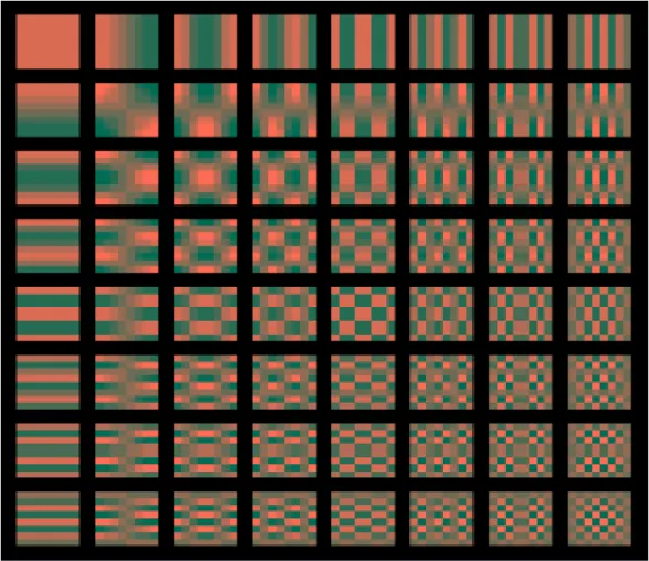
Again, it is common to depict the different cosine functions considered by the 2-dimensional DCT as a set of basis images. A set of basis images (for use with a 2-dimensional DCT operating over data blocks of 8x8 pixels) are shown in figure 9. It can be seen that the top left basis image is the DC component (i.e. there are no horizontal or vertical frequencies present in this component at all), and the bottom right basis image contains high horizontal and vertical frequencies.

(48)

All the other components contain various combinations of horizontal and vertical frequencies based on their position within the figure.

Using suitable weights to combine these basis images it is possible to create any set of 8x8 pixels.

Figure 9: basis functions used by a DCT, being calculated over a 2-dimensional data series of 8x8 samples.

As mentioned above, DCTs are commonly used in lossy compression

techniques applied to digital media. As such, much research has been carried out into efficient implementations of the DCT. For example Ananthashayana et. al. developed a novel, recursive, multiplierless algorithm for calculating 2-dimensional DCTs [40]. This algorithm can be implemented using only addition and shifting. Other work includes the development of high performance

algorithms for calculating 2D DCTs, specifically targeted at GPU architectures [29].

(49)

2.3.5 Gaussian Mixture Models

A normal or Gaussian distribution is a continuous probability distribution. It is commonly used to model the behaviour of random variables whose distributions are not known, and (in its simplest form) is described by equation 2.12.

𝑓(𝑥, 𝜇, 𝜎) = 1 𝜎√2𝜋 𝑒

−(𝑥−𝜇)_2𝜎22

(2.12) Where: f is some random variable over x.

𝜇 is the mean of the distribution

𝜎 is the standard deviation of the distribution.

The Gaussian distribution takes the form of a bell curve (as can be seen from either of the two curves shown n Figure 10). If 𝜇 = 0 and 𝜎 = 1 then the distribution can be called the standard normal distribution.

Many situations can be modelled using Gaussian distributions, and once suitable values for 𝜇 and 𝜎 have been found, the distribution can be used to better understand the origin of previously unobserved data points on the same axis.

For example, consider a target shooting game at a fair ground. Players aim at, and try to hit a target, in order to win some prize. To make the example more straightforward we will consider the player can only adjust their aim in the horizontal direction, and that the aim in the vertical direction is fixed.

Consider that two players each play the game a number of times. Each time they fire at the target they hit somewhere along the horizontal axis, but at the correct height (as this is fixed in our example). They each record their results, and we end up with two sets of data, each belonging to a different player.

After playing the game a number of times they calculate the mean, variance and standard deviation of the data, and then plot a Gaussian distribution on a graph, with probability of result shown on the y-axis, and distance from centre of target on the x-axis. It is supposed that x=0 marks the central location on the target.

(50)

Figure 10 shows what this (fictitious) graph might look like. Some anecdotal information can be extracted from the plot;

 player one (represented by the green curve) demonstrates a more consistent set of results, but their distribution is not central. Perhaps this suggests that they were possibly the more skilful player, but that they may have done better by adjusting their sight.

 player two (represented by the red curve) seems to be the less skilful player, but has a much more centrally distributed set of results.

Figure 10: Example showing the shape of two Gaussian distributions, which have different values for mean and standard deviation.

Now, if one of the two players (selected at random) plays the game again, and records their new result, we can use the plot in Figure X to work out the probability that either player was the shooter.

For example, if the record result was -1, it is unlikely player one was the shooter. However, if the result was 0.5, it is likely (but not certain) that player one was the shooter.

Using a Gaussian distribution in this way might allow some simple situations to be modelled, but generally situations are not this straight forward, and might

(51)

need a more complex distribution to provide a good fit between the model and the observed data.

For example, what would happen if (instead of trying to work out which player was the shooter in a given instance) we now want to find the probability that a given location on the target would be hit, if player one and player two are the only players? A Gaussian Mixture Model can be used to investigate this more complex situation.

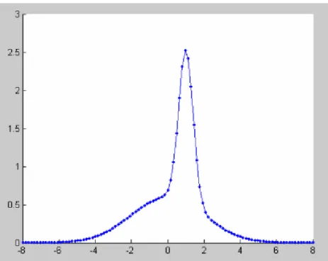
In a Gaussian Mixture Model, two or more distributions are combined in a linear and weighted manor). This is shown in equation 2.13.

𝑝(𝑥) = ∑ 𝑤_𝑗. 𝑓(𝑥, 𝜇, 𝜎)

𝐾 𝑗=1

(2.13) Where p(x) is the probability of x.

K is the number of distributions being combined in the model.

Wj is the weighting applied to distribution j.

So in the example, a weighting might be applied to each player which is proportional to how often they play the game. If player two (represented by the red distribution in figure 10) played the game twice as often as player one, then the combined probability distribution might look something that shown in figure 11.