Department of Cybernetics
Bachelor Project
Image Captioning with
Convolutional Neural Networks
Michal Najman
Supervised by Dr. JuhoKannala
and
prof. Ing. Jiˇr´ıMatas, Ph.D.
Department of Cybernetics
BACHELOR PROJECT ASSIGNMENT
Student: Michal N a j m a nStudy programme: Cybernetics and Robotics
Specialisation: Robotics
Title of Bachelor Project: Image Captioning withConvolutionalNeuralNetworks
Guidelines:
1. Familiarize yourself with neural networks and the problem of image captioning, in particular [1] and [2].
2. Reproduce some of the results of [2], evaluate the performance of the method and analyze its weaknesses.
3. Suggest improvements and evaluate them experimentally.
4. Discuss the results, their impact and potential topics for future research.
Bibliography/Sources:
[1] Ian Goodfellow, Yoshua Bengio and Aaron Courville - Deep Learning - Book in preparation for MIT Press, 2016, http://www.deeplearningbook.org
[2] Johnson, Justin and Karpathy, Andrej and Fei-Fei, Li - DenseCap: Fully Convolutional Localization Networks for Dense Captioning - Proceedings of the IEEE Conference on Computer Vision and Pattern Recognition, 2016
[3] Karpathy, Andrej and Fei-Fei, Li - Deep Visual-Semantic Alignments for Generating Image Descriptions - CoRR, 2014
Bachelor Project Supervisor: Dr. Juho Kannala
Valid until: the end of the winter semester of academic year 2017/2018
L.S.
prof. Dr. Ing. Jan Kybic
Head of Department
prof. Ing. Pavel Ripka, CSc.
In this thesis, we elaborate on image captioning concerning especially dense image cap-tioning. We present technical fundamentals of a model striving to solve such a task. Concretely, a detailed structure of DenseCap and Neural Image Caption is discussed. Experimentally, we examine results of DenseCap and analyse the model’s weaknesses. We show that 92% of the generated captions are identical to a caption in the training set while the quality of those and the novel ones remains the same. We propose a criterion that significantly reduces a set of captions addressing an image whilst SPICE score of the set is maintained.
Keywords: image captioning, dense captioning, convolutional neural networks, long short-term memory
Abstrakt
Tato bakal´aˇrsk´a pr´ace se zamˇeˇruje na automatickou tvorbu popisu obr´azk˚u (angl. im-age captioning), konkr´etnˇe na tzv. dense captioning. Problematika je uk´az´ana ve svˇetle souˇcasn´ych model˚u se zamˇeˇren´ım na stavbu DenseCap a Neural Image Cap-tion. DenseCap zejm´ena je prodoben experiment˚um, d´ıky nimˇz jsou identifikov´any nedostatky modelu. Pokusy ukazuj´ı, ˇze 92 % generovan´ych popisk˚u je identick´ych vzork˚um v tr´enovac´ı mnoˇzinˇe. Je zjiˇstˇeno, ˇze jejich kvalita v porovn´an´ı s tˇemi, kter´e v tr´enovac´ı mnoˇzinˇe nejsou, je stejn´a. V neposledn´ı ˇradˇe je navrˇzeno krit´erium, pomoc´ı nˇehoˇz lze v´yznamnˇe zmenˇsit mnoˇzinu popisk˚u vztahuj´ıc´ıch se ke konkr´etn´ımu obr´azku, kdy SPICE sk´ore t´eto menˇs´ı mnoˇziny z˚ust´av´a stejn´e.
Kl´ıˇcov´a slova: automatick´a tvorba popisu obr´azk˚u, dense captioning, konvoluˇcn´ı neu-ronov´e s´ıtˇe, long short-term memory
ˇ
Cesk´y n´azev: Automatick´a tvorba popisu obr´azku pomoc´ı konvoluˇcn´ıch neuronov´ych s´ıt´ı
I declare that the presented work was developed independently and that I have listed all sources of information used within it in accordance with the methodical instructions for observing the ethical principles in the preparation of university theses.
Prague, January 9, 2017
I gratefully thank my supervisor Dr. Juho Kannala for his wise and critical comments as well as for his enriching attitude. Kiitos! Also, my appreciation goes to prof. Ing. Jiˇr´ı Matas, Ph.D. who joined the thesis meetings and contributed immensely with novel ideas.
Last but not least, I thank my family for their support and my girlfriend Barbora for selecting the most pleasant shade of orange advisedly and for reviewing this text thoroughly.
1 Introduction 1
2 Neural Networks 5
2.1 Perceptron . . . 5
2.2 Multi-Layer Neural Network . . . 5
2.2.1 Fully Connected Layer . . . 6
2.2.2 Number of Parameters . . . 7
2.2.3 Hornik’s Theorem . . . 8
2.2.4 Name Origin . . . 8
2.3 Deep Learning . . . 8
2.4 Convolutional Neural Networks . . . 9
2.4.1 Receptive Field . . . 9
2.4.2 Convolution in CNNs . . . 10
2.4.3 Pooling Layer . . . 10
2.5 Recurrent Neural Networks . . . 11
2.5.1 Long Short-Term Memory . . . 11
3 Related Work 13 3.1 Models History . . . 13
3.2 Current Models . . . 14
3.2.1 Image Classification . . . 14
3.2.2 Object Detection . . . 14
3.2.3 Recurrent Neural Networks . . . 14
3.2.4 Metrics and Challenges . . . 14
4 Image Captioning Model 17 4.1 Image Encoder . . . 18
4.1.1 Transfer Learning . . . 18
4.1.2 VGG-16 and Inception V3 . . . 19
4.2 Salient Region Detector . . . 19
4.2.1 From Anchor to Region Proposal . . . 20
4.2.2 Region Feature Map . . . 21
4.2.3 Recognition Network . . . 22
4.3 Language Model . . . 22
5 Experiments 25 5.1 Dense Captioning Results . . . 25
5.2 Caption Quality . . . 27
5.2.1 Pascal 50S Dataset . . . 27
5.2.2 Evaluation Metrics . . . 28
5.2.3 Nearest Caption Analysis . . . 29
5.3 Beam Search . . . 30
5.4 Distinct Caption Set . . . 32
5.4.2 Caption Distinctness Predictor . . . 34 5.5 Discussion . . . 34 6 Conclusions 37 References 39 List of Figures 45 List of Tables 47 x
1
Introduction
For most computer vision researchers the classification task has always been dominant in the field. Either it was a scene understanding in the pioneer 1960s or a traffic sign detection in the modern days, the task has been rooted in the soil of computer vision. It is not surprising that one of the most significant competition in the field comprises the image classification task among others.
The ImageNet Large Scale Visual Recognition Challenge (ILSVRC) awards annually the algorithm which is most successful at predicting the class of an image in its five estimates (known as top-5 error). For the record, the lowest top-5 classification error reached 28.2% at the ILSVRC2010 and 25.8% a year later, respectively [1].
Nonetheless, an unxpected breakthrough came in the year 2012 when Krizhevsky et al. [2] presented decades old algorithms [3, 4] enhanced by novel training techniques achieving so-far-not-seen results. In particular, the top-5 classification error was pushed to 16.4%. At the latest contest in 2015, the lowest top-5 error was brought to 3.5%, drawing on the work of Krizhevsky et al.
After this success, neural networks has revolutionised the field and brought in new challenges that had not been merely considerable before. One of those newly feasible techniques – image captioning – is discussed in this thesis. In fact, as an arising discipline with promising potential, image captioning still is an active area of research nowadays, striving to answer unsolved questions. Consecutively, since the field has not been entirely established yet, one must rely mainly on recently published papers and on-line lectures only.
Considering recent work, we define image captioning as a task in which an algo-rithm describes a particular image with a statement. However, it is expected that the statement is meaningful, self-contained and grammatically and semantically correct. In other words, the caption shall describe the image concretely, shall not require or rely on additional information and, last but not least, be consisted of a grammatically correct sentence that semantically corresponds to the image.
The reader is advised to fully appreciate the complexity of this problem. Note that an image can be thought of as an vector in a million dimensional space. For a three-channel 1024×768 image, its dimensionality reaches nearly 2.4 million. This extensively long vector is then mapped into a space of statements, expecting to meet requirements set above. The notion is illustrated more concretely in Fig. 1.
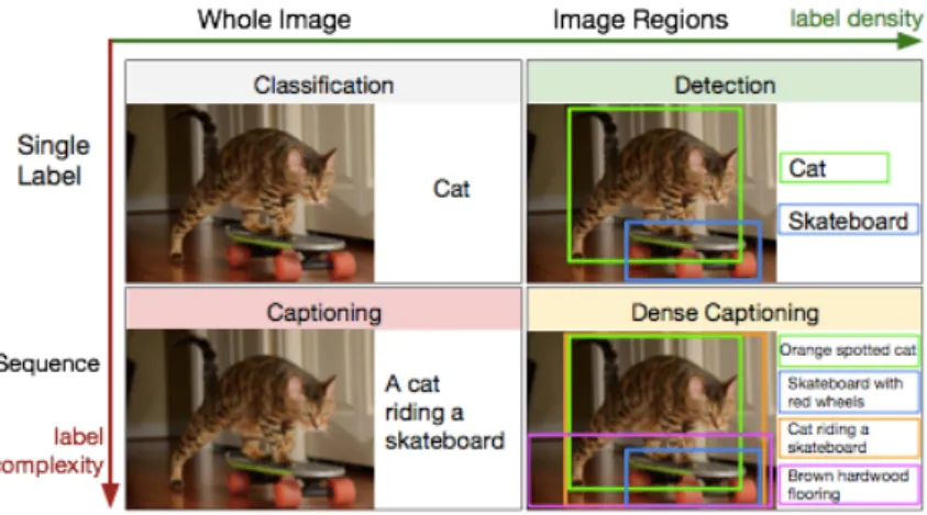
Based on full-image captioning research, in their work Johnson et al. [5] propose that the image captioning task can be viewed as weak classification since a caption is a label expressing richer concepts. Recent work in object detection enabled correct identification of multiple salient regions in an image and, similarly, rapid progress in image captioning extended the complexity of generated statements referring to an image. Therefore, Johnson et al. argue the recently seen fruitful advances in image captioning were excited along two axes — label density and label complexity. Naturally, a new unifying task they called dense captioning has arised [5]. See Fig. 2 elaborating on the notion of dense captioning.
In dense captioning, an algorithm detects salient regions in an image and captions each of those regions separately as in image captioning. Thus, the dense captioning
Image Captioning with Convolutional Neural Networks
task consists of two joint subtasks: object detection and captioning of those objects. Although the dense captioning task raises new challenges, and thus is examined in this thesis, only Johnson’s work regards it as the paper presenting the task was published only recently. Therefore, when comparing, this thesis takes into account full-image captioning mostly.
In conclusion, recent development in research utilizing accomplishments of neural networks creates a challenging opportunity of following the most up-to-date advances in image captioning while putting those notions into perspective with previously published results.
In this thesis, we examine and elaborate on the recent development in image cap-tioning, especially concerning the latest work of Johnson et al. [5], the DenseCap model, and Vinyals et al. [6], Neural Image Caption (NIC).
First, we elaborate on neural networks and deep learning, yearning to describe thoroughly the notions in relation to image captioning. In Sec. 3, influential work as well as state-of-the-art models are put into perspective with available datasets and evaluation functions. As already mentioned, the thesis regards mainly the models DenseCap and NIC whose detailed examination can be found in Sec. 4.
The results of DenseCap are discussed in Sec. 5 together with a detailed analysis of the model’s drawbacks. Following the findings, we propose experiments improving the model’s results and evaluate them.
Figure 1: When developing an automatic captioner, the desired behaviour is as follows: an image, which to a computer is a 3×W×H tensor containing integers in range from 0 to 255, is described with a sentence, which is just an ordered sets of pre-defined tokens. To illustrate the difficulty of the task, we use the famous inscription written in Black Speech that is engraved in the One Ring from the Lord of the Rings trilogy. Assuming the reader does not speak fluent Black Speech, this motivates the notion of translating a tensor into a sequence without further understanding of any of the two concepts. Essentially, we argue, this is the image captioning task.
Figure 2: In this picture, recent progress in image description is shown as improvement along two axes. From classical one-label classification new tasks have emerged — salient object in the image are labeled independently and, in contrast, labels have been extended into sentence-like captions. We define dense captioning by combining the two. Image taken from [5]
2
Neural Networks
In order to tackle the image captioning task, recent work shows it is in one’s interest to utilize neural networks [7]. This frequently used term dates back to 1950s when notions such as the Perceptron Learning Algorithm were introduced [8]. Modern neural networks draw on notions discovered in the era of a Perceptron. In this section, we first define a neuron as a fundamental part of modern neural networks. Then we elaborate on Convolutional Networks and Recurrent Networks.
2.1 Perceptron
For the purposes of this work, a perceptron is defined generally as it became a funda-mental part of modern neural networks and the notation is utilized further on. Thus, a perceptron is compounded of one neuron. The neuron’s output, known as the activation
a, is mapped by Φ :RN →Ras follows:
a= Φ(x) =σ(wTx+b) (1)
wherex∈RN is a feature vector,w∈RN andb∈Rare weights andσ(·) is a non-linear
function. In case of the Perceptron,σ(·) stands for
σ(z) = (
1 ifz >0
0 otherwise (2)
In other words, a perceptron is a non-linear function separating data into two classes each associated with either 1 or 0. A perceptron is parametrized by weights wand b. By setting proper weights, one effects the output and the perceptron’s behaviour for a given feature vector. Therefore, such weights trimming is essential, yet non-trivial task. In order to find the weights, a learning algorithm was introduced, named the Perceptron Learning Algorithm [8]. This algorithm has a limiting property such that successful learning is achieved if and only if the data are linearly separable which is a major drawback pointed out in by Minsky and Papert in 1969 [9]. For example, there is no vectorwand bias bthat would make a perceptron mimic the XOR function.
2.2 Multi-Layer Neural Network
Taking the perceptron as inspiration, the XOR problem can be overcome by aligning neurons into layers and interconnecting those layers. This function is called a Feedfor-ward Neural Network, an Artificial Neural Network or simply a Neural Network.
In a neural network, each layer comprisesN neurons processing inputs coming from the previous layer and producing activations used later in the following layer. For the sake of simplicity, it is now assumed that the number of neurons N is same for all layers. However, this varies very often, for example, usually the output layer consists of fewer neurons corresponding to the nature of the problem being solved. To conclude, the activations of thek-th layer (a(1k), a2(k), . . . , a(Nk)) =a(k)∈
Image Captioning with Convolutional Neural Networks
the activations of the previous layerk−1, noted as a(k−1)∈RN:
a(1k) = Φ(1k)(a(k−1)) a(2k) = Φ(2k)(a(k−1)) .. . a(Nk) = Φ(Nk)(a(k−1)) (3)
where Φ(ik)(·) is a function defining the properties of the i-th neuron in the layer k, often having the form similar to Eq. (1). However, there are exceptions that proved to be essential to modern neural networks designs [2, 7, 10–12]. We discuss these in the later sections.
In practise, to lower the complexity of a network, in the given layerkall the functions Φ(ik)(·) are always of the same form, only distinct in weights. Therefore, it is convenient to use vector notation. This is done by simplifying Eq. (3) into the following form:
a(k) =Φ(k)(a(k−1)) (4)
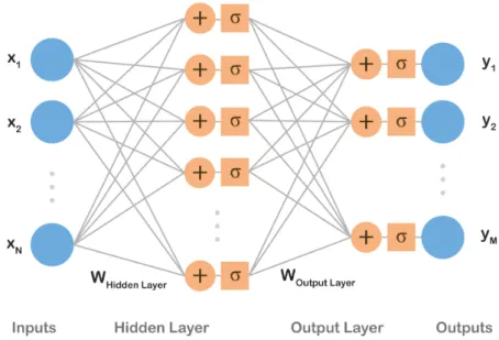
As an example, we show a neural network with one hidden layer. The network takes in a vector that is propagated forward into the hidden layer. The processes in the hidden layer are noted here as Φ(1). Further, the activations of the hidden layer are again propagated, analogically, into the second layerΦ(2) whose activations are the output of the network. The network’s design is shown in Fig. 3. Formally, the network is fed with a feature vectorx∈RN producing a vector y∈
RM:
y=Φ(x) =Φ(2)(Φ(1)(x)) (5)
whereΦ1:RN →RH is called the hidden layer andΦ2 :RH →RM is called the output
layer. Note that the number of neurons in the hidden layer H is a hyper-parameter. Although the structure of the network in the example has been defined, there are still other hyper-parameters to be determined. For example, the form of the layer mappingsΦ(1)and Φ(2) needs to be specified. A layer with the most simple form of its mapping is called a Fully Connected Layer and is discussed in the following subsection. 2.2.1 Fully Connected Layer
In the most basic neural network — a feedforward neural network comprising fully-connected layers only – each neuron processes activations of all neurons in the previous layer and is activated using Φ(·) defined in Eq. (1). Thus, based on vector notation in Eq. (4), the activations of the k-th fully-connected layer are defined as
a(k)=σ(W(k−1,k)a(k−1)+b(k−1,k)) (6) where W(k−1,k) ∈
RN×N is a weights matrix with weights vectors aligned in rows,
b(k−1,k) ∈RN is a vector of biases and σ :
RN → RN is a non-linear function. Note
that, since in practise the elementsσi(·) are identical single-variable functions, we refer
to them as simplyσ(·).
Figure 3: Inputsx1, . . . , xN are processed by a hidden layer and, consecutively, by an output
layer producing outputsy1, . . . , yM. Biasesbwere omitted for the sake of simplicity.
In contrast to a perceptron,σ(·) is generally required to be differentiable due to the nature of learning algorithms used in the field. For example, σ(·) used to be set to a sigmoid curve as similar to the perceptron’s activation fuction shown in Eq. (2). Most commonly, tanh() or the logistic function (Eq. (7)) were used.
σ(z) = 1
1 +e−z (7)
Nevertheless, when used in deep learning sigmoids suffer from problems such as vanishing or exploding gradients, therefore those were replaced with a Rectified Linear Unit (ReLU) [13]:
σ(z) = max(0,z) (8)
In modern networks, it is recommended to use ReLUs as they proved to provide better results and are thus the most common activation function used nowadays [7].
Drawing on the example presented above, we now assume that both layers are fully connected, meaning that layer mappings have a form of Eq. (6). Then Eq. (5) can be rewritten as follows:
y=σ(W(1,2)σ(W(0,1)x+b(0,1)) +b(1,2)) (9)
2.2.2 Number of Parameters
Let us now assumex∈ RN, the activations of the hidden layera ∈RH and y∈ RM.
Then we can calculate the number of parameters asN+N×H+H+H×M. Considering a small gray-scale image, 28×28, of a hand-written number taken from the MNIST dataset [14], that is classified as 0-9 digit,N = 784 andM = 10. Then the number of
Image Captioning with Convolutional Neural Networks
parameters, needed to be learned, is 795×H+ 784 where H, the number of hidden layers, is a hyper-parameter. For a hidden layer having the same width as the input vector, i.e. H= 28 in this example, the number of parameters reaches 23,044.
Truly, this is a large number for such a shallow network suggesting that fully con-nected layers extensively increase the number of parameters.
2.2.3 Hornik’s Theorem
The network mentioned above is a common design that in past was believed to yield promising results. It was shown by Hornik [15], a multilayer feedforward neural network is able to approximate any continuous function that is bounded. Yet, a possibly great number of hidden neurons might be needed in order to do so because the theorem does not quantify this important hyper-parameter.
2.2.4 Name Origin
As shown in Fig. 3, the structure is called a network since it can be drawn as a directed acyclic graph. Wondering about the name’s background, one may notice the wordneural and mistakenly assume a relation to biological neurons. However, as stated for example in [7], it is a common misconception as the name, neural networks, was derived in 1950s from former biological models serving as motivation. Those models are now, however, considered outdated, and conversely, modern neural networks are not designed to be realistic models, rather going beyond neuroscience perspective. Since that, endeavours to infer an algorithm from the brain’s functioning have not faded. For example, Jeff Hawkins et al. developed Hierarchical Temporal Memory (HTM) [16] as a strict mathematization of human neocortex based on current neuroscience. Internally, HTM as a biologically inspired algorithm is distinct from deep learning and, admittedly, its results have not been as fruitful as those obtained by deep nets [17], which are discussed int the following section.
2.3 Deep Learning
In spite of former beliefs, it was found that [7] it is more efficient to insert several hidden layers one by one and propagate information sequentially creating a deep structure, instead of utilizing a shallow network given in the example. This concept is called deep learning and, surprisingly, has its roots already in the pioneer 1960s as it was assumed that an intelligent algorithm solving complex problems shall work with hierarchy of concepts [7] that was rather deep. This is why we get the name deep learning.
The notion was later found in the idea of modern neural networks which, as stated above, consist of numerous nested layers each extracting more abstract and complex features as information is propagated forward the network. Therefore, the modern neural networks and techniques used for learning them are usually nowadays referred to as deep learning.
Deep neural networks were introduced already in 1998 [18] and the optimization algorithm (back-propagation) was known by then and used frequently [3]. Yet, the deep nets were found too complex to be trained. In their books, Ian Goodfellow et 8
al. list those reason that enabled the boom of neural networks in 2012: firstly, more data were available as well, therefore, the deep nets have started to outperform other models. Secondly, deeper models require decent architectures both in software and hardware and those had become available. Then on, promising results enabled advent of neural networks, especially in their deep form. Models such as convolutional neural networks or recurrent nets are considered state-of-the-art building blocks nowadays. Their detailed design is discussed in the following subsections.
2.4 Convolutional Neural Networks
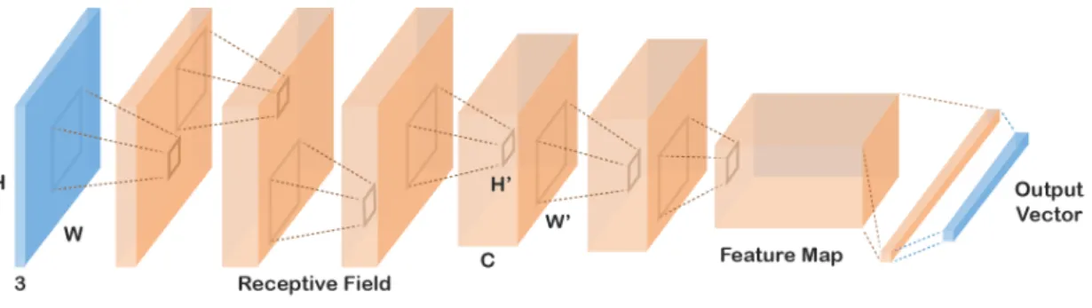
In image analysis, many of recent advances in deep learning are built on the work of LeCun et al. [18] who introduced a Convolutional Neural Network (CNN) which had a large impact on the field. A CNN is a type of a neural network that is designed to process an image and represent it with a vector code. The architecture of CNNa draws on fully-connected neural networks. Similarly, a convolutional neural network is a compounded structure of several layers processing signals and propagating them forward.
However, in contrast to a vector activation in a fully-connected layer, activations in CNNs have a shape of three-dimensional tensors. Commonly, this output tensor is called a feature map. For instance, an input image of shape 3×W ×H is transformed by the first convolutional layer into a feature map of shape C×W0×H0, where C is the number of features. In other words, a convolutional layer transforms a volume into a volume.
A typical CNN consists of several convolutional layers and, at the top, fully con-nected layers that flatten convolutional volumes into a vector output. In the field’s terminology, this vector code of an image is often called fc7 features as it used to be extracted from the seventh fully connected layer of AlexNet [2]. Even though AlexNet has already been outperformed by many and the state-of-the-art designs are different from AlexNet, the term maintained its popularity. Additionally, depending on a prob-lem the network is supposed to solve, an additional layer, such as soft-max, can be added on top of fc7 features. A common design of a CNN is depicted in Fig. 4 2.4.1 Receptive Field
As mentioned above, a convolutional layer takes a tensor on input and produces a ten-sor, too. Note that these tensors have two spatial dimensionsW andH, and one feature dimensionC as they copy the form images are stored in. The context conveyed by the spatial dimensions is utilized in the CNN design which takes into account correlations in small areas of the input tensor called receptive fields. Concretely, in contrast to a neuron in a fully connected layer that processes all activations of the previous layer, a neuron in a convolutional layer ”sees” only activations in its receptive field. Instead of transforming layer’s activations it restraints to a specific small rectangularly shaped subset of the activations. When mentioning a receptive field, it is often expected only spatial dimensions of the input volume are referred to, i.e. a receptive field defines an area in the W ×H grid. The shape of the receptive field is a hyper-parameter and varies across the models.
Image Captioning with Convolutional Neural Networks
Figure 4: A convolutional neural network takes an image on input (in blue) and transforms it into a vector code (in blue). Convolutional Neural Networks are characteristic for processing volumes. An output of each layer is illustrated as an orange volume. Each neuron process only activations in the previous layer that belong to its receptive field. The same set of weights is used for neurons across the whole grid. On top of convolutional layers, fully-connected layers are commonly connected.
2.4.2 Convolution in CNNs
A neuron’s receptive field is processed similarly to fully connected layer neurons. The values below the receptive field along the input tensor’s full depth are transformed by a non-linear function, typically ReLU (Eq. (8)).
However, in contrast to fully connected layer neurons, the same set of weights (referred to as a kernel) is used for all receptive fields in the input volume resulting into a transformation that has a form of convolution across the input. A kernel is convolved acrossW and H spatial dimensions. Then, a different kernel is again convolved across the input volume producing another 2D tensor. Aligning up the output tensors into a
C×W0×H0 volume assembles the layer’s output feature map.
This is an important property of convolutional neural networks because each kernel detects a specific feature in the input. For example, in the first layer, the first kernel would detect presence of horizontal lines in the receptive fields, the second kernel would look for vertical lines, and similarly further on. In fact, learning such types of detectors in the bottom layers is typical for CNNs.
The design of CNNs has an immensely practical implication – since a kernel is con-volved across the input utilizing the same set of weights and it covers only the receptive field, the number of parameters is significantly reduced. Therefore, convolutional layers are less costly in terms of memory usage and the training time is shorter.
2.4.3 Pooling Layer
Convolutional layers are designed in such a way the spatial dimensions are preserved and the depth is increased along the network flow. However, it is practical to reduce spatial dimensions, especially in higher layers. Dimensions reduction can be obtained by using stride when convolving, leading to dilution of receptive fields overlap. Nev-ertheless, a more straightforward technique was developed called a pooling layer. An 10
input is partitioned into non-overlapping rectangles and the layer simply outputs a grid of maximum values of each rectangle. In practise, pooling layers are inserted often in between convolutional layers to reduce dimensionality.
2.5 Recurrent Neural Networks
Convolutional and fully connected layers are designed to process input in one time step without temporal context. Nonetheless, some tasks require concerning sequences where data are temporally interdependent. For that, a Recurrent Neural Network (RNN) – an extension of fully connected layers – has been introduced. RNNs are neural networks concerning information from previous time steps .
RNNs are used in a variety of tasks: transforming a static input into a sequence (e.g. image captioning); processing sequences into a static output (e.g. video labelling); or transforming sequences into sequences (e.g. automatic translation).
A simple recurrent network is typically designed by taking the layer’s output from the previous step and concatenating it with the current step input:
yt=f(xt,yt−1) (10)
The function f is a standard fully-connected layer that processes both inputs indis-tinctly as one vector. Due to its simplicity, this approach is rather not sufficient and does not yield promising results [19]. Thus, in past years, a great number of meaningful designs have been tested [20]. The notion was advanced and designs have become more complex. For example, an inner state vector was introduced to convey information between times steps:
ht,yt=f(xt,ht−1) (11)
The most popular architecture nowadays is a Long Short-Term Memory (LSTM) [21] – a rather complex design, yet outperforming others [20].
2.5.1 Long Short-Term Memory A standard LSTM layer is given as follows:
ft=σg(Wfxt+Ufht−1+bf) (12)
it=σg(Wixt+Uiht−1+bi) (13)
ot=σg(Woxt+Uoht−1+bo) (14)
ct=ftct−1+itσc(Wcxt+Ucht−1+bc) (15)
ht=otσh(ct) (16)
where xt is an input vector and ht−1 is an output vector. All matrices W and U
and biases b are weights that together, with σg which is a logistic function Eq. (7),
represent a standard neural network layer.
Thus, the forget gate vector ft, the input gate vector it and output gate vector ot
are outputs of three distinct one-layer neural nets each having its output between−1 and 1. ct is a cell state vector that, as a hidden output, is propagated to the next time
Image Captioning with Convolutional Neural Networks
step. ht is an output of the LSTM cell. stands for element-wise multiplication, σc
and σh are usually set to tanh.
Note thatctis a combination of the previous time stepct−1, element-wisely adjusted
by the forget gateft, and the output of a neural network, gated similarly by the input
gateit.
The output of LSTMhtis a function of the cell state vector, first squashed between
0 and 1, and then adjusted by the output gate ot.
Connected to a network, LSTM consists typically of one layer only. LSTMs are known to preserve long-term dependencies, as shown for example by Karpathy [22].
3
Related Work
For a human, seeing an image for a short time is sufficient enough to describe it com-prehensively [23]. Humans undertake this task intuitively and can produce immensely detailed description of the image. Nonetheless, producing similar results with a com-puter has proven to be a rather difficult task.
Image description was first tackled in a classification task where a label is assigned to an image [1, 24]. Although this approach have recently reached outstanding results as mentioned in Introduction, they cannot overcome the essential limitation as their set of outcomes is predefined and thus fixed. In real-world tasks a method yearning to compete with human abilities has to be capable of working with an unlimited set of out-puts. In image captioning, such quality is especially desired as natural language, that captions are expressed with, is essentially unlimited. This fact has led to utilizing Re-current Neural Networks in numerous recent papers [6, 25–29] as they are theoretically able to process and generate any sequence.
In Sec. 3.1, the relevant models leading to modern examples are discussed. Then, in Sec. 3.2 we elaborate on the most advanced algorithms that have been developed in image captioning. The detailed structure and principles are, however, extended on in Sec. 4.
3.1 Models History
The idea of describing an image with a statement was first unfolded using hard-coded rules that specified which visual context shall be used [30]. Some of the early approaches [31, 32] targeted videos as their visual input instead of nowadays more popular images. Nevertheless, the limitation of the fixed size output set still held true.
Challenging it, some authors came up with image-sentence embeddings [33] that bound an image and a textual statement in a common space [34, 35]. Also, it was very often to view the problem as document retrieval, meaning that for a given test image, a statement is retrieved from the training dataset, on the basis of image similarity [30, 36–38]. The latest mentioned approach uncovers the potential of a baseline methodk -nearest neighbours in which the non-trivial task of finding convenient distance between images is tackled with CNNs [39]. In particular, the authors of [40] show that an image can be represented with a vector code obtained by a CNN. Image similarity is then measured in the space of those vector codes using, for example, euclidean distance. The caption is then chosen from the nearest images in the training set. In addition, some authors combine sentences stored in a database [41, 42].
After publishing their work referred to as AlexNet [2], Krizhevsky et al. were followed by many with applying convolutional neural networks to various problems. Recent work in image captioning, in particular, utilizes CNNs as image encoder [5, 6, 43, 44].
Image Captioning with Convolutional Neural Networks
3.2 Current Models
3.2.1 Image Classification
In the most recent work in computer vision, variations of neural networks trained with stochastic gradient descent [2] are mostly used. These models are trained to classify an image, i.e. assign a class label to it [3, 10]. It proved to be very efficient to utilize a pre-trained image classification model in similar tasks. [5, 6, 25, 43, 44]. From the great variety of pre-trained models, let us mention VGG-16 [10] and Inception V3 [11] that set the state-of-the-art performance. Most recently, Inception V4 was introduced proposing a new framework of a convolutional layer that adds the feature map to its input and outputs this sum.
3.2.2 Object Detection
In the dense captioning task [5], an image is described with a set of statements, each corresponding to a salient region in the image. Thus, different phenomenons present in the image need to be detected and localized in order to describe them. The most advanced methods solving such a task (object detection) draw again on CNNs, such as YOLO [45] or Fast R-CNN [46].
Lately, Ren et al. [47] focused on generating boxes with a fully convolutional network by converting anchors into region proposals (Faster R-CNN), yet they do not propose end-to-end trainable architecture. Drawing on Faster R-CNN, a model entirely trained with back-propagation has been proposed by Johnson et al., called FCLN [5]. In terms of time performance, SSD by [48] outperforms others.
3.2.3 Recurrent Neural Networks
Assuming an image have been decoded into a feature map, recent publications adopt Recurrent Neural Networks (RNNs) [27, 49, 50] to construct a language model that generates text. Ability of RNNs to preserve long-term relations and generate sequences was studied by Bahdanau et al. [51–53].
Calling on these notions, a multimodal RNN was introduced [25, 27, 44, 54]. Further work, on the other hand, simplified the language model and developed other RNN designs. Karpathy and Fei-Fei [43] exploited a Bidirectional RNN [55], whereas for example Kiros et al. [27] rather drew on the LSTM recurrence [21] by propagating the visual information from the decoder directly to the language model. Karpathy et al. [22] showed why LSTM in particular provides surprisingly good results despite their complex architecture. A certainly interesting idea was introduced by Bengio et al. [56] who took into account spatial attention – a map that highlights areas of an image that shall be described by the language model.
3.2.4 Metrics and Challenges
To measure performance of image captioning models, several metrics have been de-veloped, such as CIDEr [57], BLEU [58] or METEOR [59] that each exploits different natural language characteristics. Yet it is a commonly shared opinion that each of them 14
suffers from major drawbacks. To show that even a sufficient metric of image caption-ing is still an open problem, the reader is encouraged to consider 2015 MSCOCO Image Captioning Challenge [60] that introduced a unique human-evaluated judge system to overcome drawbacks of each automatic method. And in the post-contest evaluation, the submissions are judged with all the metrics mentioned above.
METEOR and BLEU are machine translation metrics adopted for image captioning, while CIDEr was designed to evaluate image captions. However, most recently intro-duced SPICE [61] is highlighted for its correlation with human judgements reaching 0.88 whereas CIDEr achieves 0.43.
Based on the results of 2015 MSCOCO Image Captioning Challenge, the best state-of-the-art performance was achieved equally by the Neural Image Caption model (NIC) [6] and the model presented by a team from Microsoft Research [28]. In terms of dense captioning, the best results are produced by the DenseCap model [5] which together with NIC is examined in this work further on.
4
Image Captioning Model
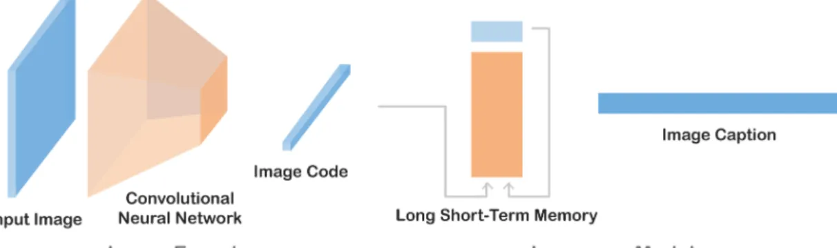
Image captioning models are complex systems that have been consisted of several mod-ules from the very beggining. Presence of modularity holds true for modern captioning models as well. Framed by Vinyals et al. [6], modern image captioning models are generally compounded of two parts: an image encoder and a language model. In this section we adapt the framework and extend it to dense captioning. The notion of modularity is shown in Fig. 5.
In other words, an image encoder takes in a raw image an encodes it into a feature map using a CNN. As there has emerged numerous CNN models in past few years, we examine VGG-16 and Inception V3 in Sub. 4.1.
Having the feature map extracted, the most recent language models generated text sequentially, word by word, relying on inherited probabilistic dependency. Therefore, given an image, a caption S having the biggest probability is expected to paint the image most accurately, i.e. S = arg maxp(Si|I).
To break this two-module scheme right away, in dense captioning a model generates text corresponding to regions in the image, therefore, such a model extends on the scheme and embeds a salient region detector in between the modules. Concretely, the region detector localizes objects in the full-image feature map and, for each, interpolates its own feature map that is further propagated into the language model. A scheme of a dense captioning model is shown in Fig. 6.
Regarding training captioning models, it is common in deep learning, models are constructed in such a way they can be trained in an ”end-to-end” fashion. End-to-end means only single loss function is used for optimizing the entire model which simplifies training significantly. This intriguing quality holds true for both examined models. Therefore, all modules of the models are optimized jointly utilizing a loss function operating over the output words. The error is back-propagated through the language model, optionally the salient region detector, down to the image encoder if fine-tuning is enabled. As a result, these modules are intertwined and non-interchangeable without further interventions.
Figure 5: An image captioning model consists of an image encoder and a language model. The image encoder transforms an image into a vector code with a CNN. The language model generates sequentially a caption conditioned on the image code.
Image Captioning with Convolutional Neural Networks
Figure 6: A dense captioning model consists of three modules: an image encoder, a salient region detector and a language model. The image encoder transforms an image into an image feature map (in blue) that is accepted by the salient region detector that localizes regions in the image using a localization layer. The language model generates sequentially a region caption conditioned on the region code (in blue) for each region separately.
In this section, we look at the architecture of image captioning models and explore and examine the most advanced two of them representing the state-of-the-art design, in particular DenseCap and NIC.
4.1 Image Encoder
Regarding an image encoder as a black box, it is fed with a raw image of shape 3×W×H
without additional pre-processing and it outputs a C×W0×H0 tensor denoted as a feature map.
4.1.1 Transfer Learning
Typically, the image encoder is a CNN architecture that has been pre-trained on a similar task concerning images, e.g. image classification. In practise, this means one chooses a particular CNN architecture from a great variety of them and removes some of the top layers of the network. In the case of AlexNet [2], it is very common to extract the features of the seventh layer (fc7features); and for example Jonhson et al. removed in DenseCap only the final pooling layer of the VGG design [10].
Since the encoder network has been trained on images, the required feature detectors at each layer has already been established. Although this is a useful trick decreasing training time, transfer learning [62] yields drawbacks — the nature of the image dataset, that the model was pre-trained on, determines what features are learnt. If the network was trained to describe significantly distinct images, the language model receives just partial information of what the given image captures. This is partially overcome by fine-tuning, which is a training phase in which the weights of the image encoder are adjusted as well, usually with lower learning rate. Concretely, in DenseCap, Johnson et al. fine-tuned all but the first four convolutional layers after 1 epoch.
Figure 7: VGG-16 [10] and Inception V3 [11] are illustrated in the figure. Note that in contrast to VGG-16 that consists of traditional convolutinal layers, Inception V3 comprises Inception blocks that each is a convolutional network. It is underlined that Inception V3 has significantly deeper structure. The ratios of the output volumes (in orange) are not preserved.
4.1.2 VGG-16 and Inception V3
CNN models differ in depth and overall design. Nevertheless, a common framework was outlined by AlexNet proposing what type of convolutional layers shall be used. The image encoders in DenseCap and Show and Tell are based on AlexNet – VGG-16 [10], and respectively Inception V3 [11], both reach impressive performance [1, 60] where the later, as of writing this thesis, is one of the most advanced CNN networks yielding in an ensemble 3.58% top-5 error on the validation set of the ILSVRC 2012 classification challenge. To compare, VGG-16 achieved 6.8% top-5 error on the same dataset.
Although detailed analysis of VGG-16 and Inception V3 goes beyond the scope of this work, we would like to point out that there is a fundamental difference between the networks. Whereas VGG-16 is constructed of traditional convolutional and max-pooling layers, Inception V3 goes beyond this framework and incorporates very deep structure of Inception blocks. The comparison of the two is shown in Fig. 7.
Having mentioned the design of the networks, the image encoder is treated in image captioning as a black box that extracts features from an image.
4.2 Salient Region Detector
This module is specific to dense captioning in terms of describing images. However, salient region detectors are essential for object detection. In this section, we describe Fully Convolutional Localization Layer (FCLN) introduced in DenseCap by Johson et al. FCLN is based on the Faster R-CNN model [47] built up for object detection. Fig.
Image Captioning with Convolutional Neural Networks
Figure 8: The scheme of the DenseCap model. Taken from [5].
8 shows that, as a black box, FCLN accepts an image feature map and returns B in-terpolated region codes of each region. B is a hyper-parameter setting the number of regions being described. In addition to the region codes, FCLN passes on four param-eters denoting a rectangular bounding box and a region confidence into the language model.
Although it is theoretically not necessary, the salient regions are considered to be rectangular as it is more convenient to pass on four parameters defining a rectangle instead of a more complex structure marking a real shape of the region. Also, the later is much harder to detect since object segmentation is considered to be a more difficult task than detection and convenient datasets have been published just recently (e.g. Visual Genome [63]).
4.2.1 From Anchor to Region Proposal
In FCLN, an approach similar to Faster R-CNN is utilized to predict region proposals. For each point in the W0 ×H0 grid, a corresponding point in the image is found, i.e. the grid W0 ×H0 is stretched out onto the W ×H grid. k default anchors of various aspects ratios are assigned to each mapped point in the stretched out grid, creating kW H0 anchor boxes distributed regularly across the image in groups of k. Since FCLN regresses each region proposal on its anchor independently, this method is translation invariant to the actual position of objects in the image which, indeed, is a very convenient property.
The regression in particular is done as follows: the image feature map is transformed by a CNN into a 5k×W0×H0 tensor containing four bounding box coordinates and a confidence score of each region proposal – five numbers per anchor, hence 5kW0H0 in total.
In FCLN, the box coordinates parametrize a region with respect to its anchor’s 20
default position and aspects. In order to define the bounding box in the 0−1 interval, the parametrization exploits normalized offset and log-space scaling transformation adapted from [46]. The confidence score denotes objectness of the captured area in the region and, thus, evaluates the content of the bounding box.
The extensive number of region proposals needs to be subsampled. Once the region proposals have been obtained, B of them are sampled using greedy non-maximum suppression (NMS) and the confidence score at test time.
To conclude, the CNN regresses bounding boxes and confidence scores from an image feature map. Due to the extensively large number of region proposals, onlyB of them are sampled.
4.2.2 Region Feature Map
Having the bounding box generated, a feature map for each individual region needs to be projected from the full-image feature map. To do so, Faster R-CNN sets in an RoI pooling mechanism. The RoI layer is proposed in such a way back-propagation is exploitable only for the weights of the image decoder, but not for the CNN that transforms coordinates and scores. In Faster R-CNN they overcome this with instead developed four-step optimization process which the detector is trained with.
To extend on that, the subtask is defined as follows: given the coordinates of the region and theC×W0×H0 image feature map, extract aC×X×Y region feature map, where X and Y are fixed, thus independent on actual dimensions of the region. The given subtask is not trivial due to regularity of the grid, where its dimensionsX, Y and the dimensions of the region proposal are generally incommensurable – we transform a variable rectangular area of W0 ×H0 into a fixed grid X×Y. In Faster R-CNN, they solve the problem with grounding which is a non-differentiable function, thus an obstacle for back-propagation.
In contrast, Johnson et al. overcame this method with bilinear interpolation which is the main contribution of FCLN, enabling the DenseCap model to be trained in an end-to-end fashion.
Intuitively, the full-image feature map is cropped at the real-valued area of the bounding box, stretched out and ”averaged” so that only corresponding areas of the
W0×H0 grid are mapped into the X×Y grid.
Concretely, if we denote a full-image feature mapC×W0×H0 by a tensorU and a region feature mapC×X×Y byV, FCLN interpolation U →V is defined as follows:
Vc,i,j = W0 X i0=1 H0 X j0=1
Uc,i0,j0 ·k(i0−xi,j)·k(j0−yi,j) (17)
wherexi,j andyi,jare real-valued coordinates inU so thatVc,i,jshould be equal toU at
(c, xi,j, yi,j). xi,j andyi,j are computed based on dimensions and position of the region
proposal. Computation of xi,j and yi,j is an essential step in projecting the region
proposal to U and stands for the ”cropping and stretching” part of the process. The ”averaging” part is done by bilinear interpolation where kernelk(d) = max(0,1− |d|) is used.
Image Captioning with Convolutional Neural Networks
To sum up the projection step, the values of theX×Y grid are a linear combination of the corresponding values of the W0 ×H0 grid whilst the number of features C is preserved.
4.2.3 Recognition Network
Lastly, to reshape the tensor into a vector and provide additional transformation, a Recognition Network is connected to the output of FCLN. This two-layer fully con-nected neural network serves as a utility reshaping the region feature map tensor into a D-dimensional code representing the region. Also, such transformation is applied to the bounding box parameters and the confidence score. Johnson et al. argue this refines the required values needed in the language model.
4.3 Language Model
For generating text, a language model conditioned on the region codes is used in both DenseCap and NIC (where a full-image code is accepted instead). In fact, these models are merely identical regarding text as a sequence of tokens from a pre-defined vo-cabulary. When working with sequences, recurrent neural networks [39], the LSTM recurrence yields best results in cases of processing language [22]. It is no wonder this rather complex architecture was chosen for its performance in both examined models.
The sentenceSthat is to be generated consists ofT words creating a chains1, . . . , sT
where each word is an element of the vocabulary V. The generative process starts with the region code obtained from the previous module. The code is transformed additionally to a smaller sized vector and fed into the LSTM at the zero time step.
x0=W(region code) (18)
y0=LST M(x0) (19)
whereW is the down-scale transformation of the region code.
The zero time step initializes hidden states, therefore, the output of LSTM y0 is
discarded. After it, x1 is set to a specialSTART token that is passed on to the LSTM
which, in contrast to the zero step, now generates the token the first word is chosen from.
y1 =LST M(x1) (20)
Now on, at every time step,ytis regressed to a word st∈V. After selecting the word
st, the tokenxt+1 corresponding to this word is inputted again into the LSTM at time
t+ 1, creating a loop. This process repeats on, until theEND token,yT, is obtained on
the output of the LSTM. Note that every sentence has a different length, therefore, T
just denotes the times step in which theENDtoken was sampled.
Regressing st on yt is not a trivial task. Both NIC and DenseCap utilize a
soft-max layer that estimates probabilities of each word from V given yt. In DenseCap,
st is sampled greedily meaning that at each time step t, the word having the highest
probability is chosen, i.e. st = arg maxsi∈V p(si) where p(si) is the probability of the wordsi at the time stept.
Yearning for more sophisticated results, NIC extends the regression by maximizing the probability of the whole sentence S. It is assumed the optimal sentence S∗ is given byS∗= arg maxSp(S), and the probability of the sentenceS is given by p(S) =
p(s1)·. . .·p(sT). Sampling the words greedily, as it is done in DenseCap, does not
guarantee bringing in the optimal solution. For that reason, NIC employs the beam search algorithm that, at every time step, keeps inl sequences of words that have the highest probability. Beam search does not guarantee finding an optimal solution either but surely can generate more likely sentences. In fact, in the latest NIC paper [6], they report that their model yields best performance whenl= 3.
5
Experiments
Having stated the fundamentals of image captioning models, this section presents the experiments conducted to verify hypotheses regarding their performance. It is impor-tant to underline the fact that improvement is traceable as long as there is sufficiently defined evaluation function. In the problem of dense captioning, there are several as-pects to be measured. Namely, a generated bounding box shall be positioned correctly and a caption shall be well-written and meaningful. Note that the later is defined vaguely and, thus, needs to be specified (caption quality is discussed in Sec. 5.2).
Although immense progress in the field has been seen lately, there is still notable dependency on computational power when applying changes to a model. Thus, when drawing up this thesis it was right away determined that all possible experiments trig-gering with weights in the model are, unfortunately, infeasible if one seeks to ehnance model’s performance significantly using an average computer. To illustrate the fact, Vinyals et al. [6] state that training the NIC model took over three weeks with a high-end GPU and, similarly, Johnson et al. [5] report the DenseCap model generates 100 captions in 166ms using a single GPU whereas the same task is done on our machine in 31s running on CPU (190× slower). From that reason, experiments that require re-training, i.e. modifying a localization layer in DenseCap, were omitted.
Further, Hessel et al. show that the failing cases of image captioning have its roots in the language model [64]. They report that training the image encoder gradually, while keeping the same language model, improves the results at every step. Conversely, while fixing the image encoder, training the language model yields better captions to a certain level after which additional training does not improve the results. They argue the finding suggests that the current language models are the core limitation.
Therefore, we focused the experiments on quality of captions where we see a room for improvements. As an experimental model, DenseCap is used since its authors made their pre-trained model available on-line [65].
5.1 Dense Captioning Results
Given an imageI, the DenseCap model generates a set of captionsCwhere each caption
c∈C is associated with its bounding box b= (x1, y1, x2, y2) and a region confidence
score s. During our experiments, we set the number of generated captions B = 300 while we consider only those of them whoses >−4, leading to C ≈150 on average.
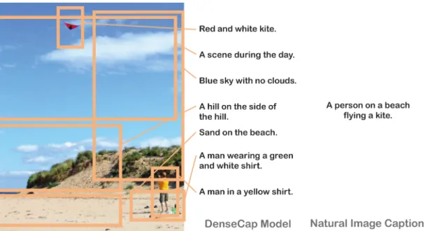
A typical result of DenseCap and NIC is shown in Fig. 9. The most significant distinctness of the models is their output – a caption in contrast to a set of captions. Therefore, the nature of generated text is different. Concretely, covering the example image, the NIC model captions the scene generally whereas DenseCap detects each salient region (the kite, the person, the sand, the blue sky and others) and captions them separately. More information is found using the later approach, for example, the color of the t-shirt, the sky, the trees on the hill.
The reader is encouraged to appreciate the quality of the generated captions as this performance was far from achieving no more than three years ago. Yet, in the following pages we examine drawbacks of the DenseCap method.
Image Captioning with Convolutional Neural Networks
Figure 9: Note that NIC captions the image generally relating to important phenomenons in the image whereas each caption of DenseCap corresponds to a salient region in the image. The captions shown were cherry-picked from a set of 153 captions to illustrate the performance. The image is taken from [66].
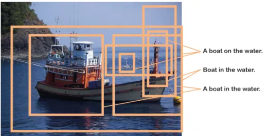
Redundancy We found that the set of captions C is redundant and contains a rel-atively big number of identical captions in terms of textual similarity (shown in Fig. 10), thus it is relevant to reduce the set while maintaining the conveyed information, see Sec. 5.4.
Restricted Outcomes Concerning generated statements, we found that only a lim-ited number of words from the training vocabulary is retrieved. Concretely, the model was trained on a vocabulary containing 11 thousand words, whereas the set of words generated on the test set (Pascal 50S) was significantly smaller, concretely 719 words. In addition, in Sec. 5.2.3 we show that 92% of the generated captions are identical to the training samples.
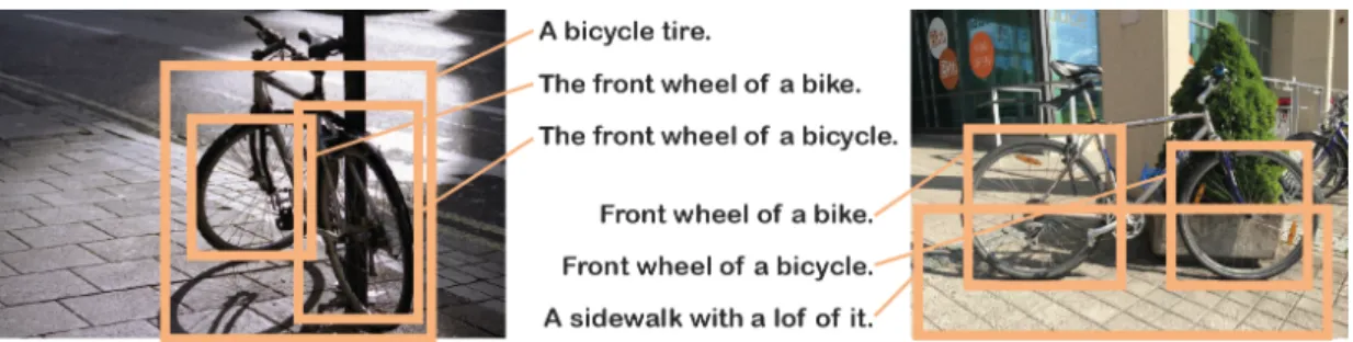
Scene Setting Dependency Moreover, we found that the generated captions rep-resent the distribution of words in the training set but not tightly – this can be shown with articles. For example, we examined the training set distribution of the following terms: a front wheel, the front wheel, front wheel. The term front wheel is by far most common. Same applies to the distribution found in pictures of front wheels of a bicycle where the termfront wheel is the most frequent one as well.
However, when the angle from which the image was taken is changed and typically the object does not face the camera directly, this distribution is affected leading to misclassification of an object. For example, we found that a bicycle that has its front wheel on the right-hand side is misclassified more often than when facing the left side. 26
Figure 10: This figure illustrates redundancy of the set of the generated captions. Note that all of the bounding boxes depicted are described with factually identical captions, only articles and prepositions differ. Additionally, some of the boxes do not overlap thus it is not possible to determine how many boats there are in the picture. Although not depicted, given this image, similar redundancy was observed with the captionBoat is white.
Also, if the bicycle is taken from the forty-five angle position, the model captions the rear wheel asfront wheel or generates meaningless captions (bike on the bike, a black metal umbrella).
The finding suggests that objects set up unusually in the scene are captioned incor-rectly or not recognised at all; and that common phrases are linked with specific object positions whereas least common or rare settings of the same objects are captioned in-correctly (see Fig. 11). In conclusion, to find the most failing case and examine their source one needs to test the model on a dataset containing unusual scene settings which is presented in the following section.
5.2 Caption Quality 5.2.1 Pascal 50S Dataset
Unfortunately, the only dataset available for dense captioning is the Visual Genome dataset that was used for training the model – the test set used by Johnson et al. is not available. We decided to evaluate caption quality on the Pascal 50S dataset [57]. Pascal 50S contains 1000 images, each captioned with 50 statements covering to the full image. Also, Pascal 50S contains images which some of them are blurred or taken from an unusual angle.
Despite dense captioning is examined, we decided to use a dataset of full-image captions. Thus, we evaluate a set of captionsC, generated given an imageI, against a ground truth setCGT that covers I.
Image Captioning with Convolutional Neural Networks
Figure 11: The figure illustrates scene dependency of DenseCap. Taking a bicycle from an unusual angle leads to misclassification. The image on the left is taken from behind and the other depicts a bike facing right-hand side – both positions are considered unusual scene settings (if the same bike is taken facing left-hand side, wheel captions are correct). Note that all wheels are captioned as a front wheel. Also, the other captions are erroneous.
5.2.2 Evaluation Metrics
In this work, SPICE [61], Levenshtein distance and sets overlap are used.
As SPICE works with semantic propositional content of a caption converting it into a scene graph, it provides more transparent evaluation than other captioning metrics, in our view. More importantly, SPICE is adaptable to dense captioning due to its properties. We propose a trick that extends its capabilities from evaluating a statement to a set of statements. In practice, this means that the set C is concatenated into a single string in which captions are separated with a dot, as in real text.
To evaluate a caption, similarity of a candidate caption scene graph and a reference scene graph is computed. In SPICE, graph similarity is given by F-score of correspond-ing edges in the graphs. Workcorrespond-ing with graphs provides convenient implications: SPICE is invariant to order and duplicity of the concatenated statements.
In conclusion, SPICE covers factual accuracy taking into account linguistic varia-tion.
Beside SPICE, Levenshtein distance and sets overlap are used in this thesis. Lev-enshtein distance denotes a minimum number of edits applied to change one statement into the other, i.e. inserting, substituting or deleting one word.
For fast evaluation, we use sets overlap. We create a set of words from each caption and exclude stop words, then we compute sets overlap as intersection over union. The set of stop words contains the most frequent words: {a, an, the, is, are, in, on, of, with, to, and}.
As shown later, it is convenient to find the nearest caption. This can be interpreted as looking for the most similar caption. This is done with both Levenshtein distance and sets overlap. In case of the former, given a set of captionsE, the nearest captions
e∗ ∈E to a caption cis defined as follows:
e∗= arg min
e∈El(e, c) (21)
wherel(·,·) is Levenshtein distance. The nearest caption for sets overlap is defined as
the captione∗ maximizing sets overlap:
e∗= arg max
e∈E s(e, c) (22)
wheres(·,·) is word sets overlap of two captions. Further on, we denote maximal sets overlap as MSO.
5.2.3 Nearest Caption Analysis
Using the Pascal 50S dataset, it was found that the generated captions are very similar to the captions in the training setCtrain. In fact, 91.94% of the generated captions are
identical to a caption inCtrain. To address the remaining 8.06% of captions, we utilize
minimal Levenshtein distance over Ctrain to find the nearest caption. In Tab. 1, the
frequency of minimal distances is shown. Note that more than 99% has a minimum distance one or zero. Examples of one-distanced captions is shown in Tab. 2.
Levenshtein Distance Frequency
0 91.94%
1 7.32%
2 0.69%
3 0.05%
Table 1: The generated captions are very sim-ilar to the examples in the training set. Nearly 92% of them are identical to some caption in the training set. Minimal distance of 1, i.e. only one word was inserted, substituted or deleted, has frequency of 7.32%. Less than 1% has a nearest distance 2 or 3. Genereated by DenseCap [5] on Pascal 50S [24].
Minimal Levenshtein distance does not provide sufficient details for captions fur-ther than 1, hence for additional analysis, we used maximal sets overlap (MSO). This measure is utilised especially when looking for the nearest caption inCGT where
Lev-enshtein reaches values beyond 5 or 6 which for a short caption often means entire sub-stitution.
Looking at the nearest captions inCGT,
we found that 35.59% of the generated captions has MSO equal to 0. On the other side of the spectrum, the captions with MSO greater than 0.5 has frequency of 1.29%. Examples of such captions and their nearest samples inCGT are shown in
Tab. 3.
To compare the sets, average MSO over Ctrain is 0.98 whereas over CGT it is only
0.14. The findings suggest that the generated captions and the ground truth captions are significantly distinct. An example ofCGT and C is shown in Fig. 14.
The following findings in this section are comprehensively depicted in Fig. 12, in which captions are compared with Ctrain and CGT, and the histograms of their
evaluation scores are shown.
We found that SPICE and MSO has correlation of 0.77 when evaluating against
CGT. Therefore, we use MSO when evaluating against Ctrain as this operation would
be very costly using SPICE. Certainly, on the other hand, SPICE as a more complex evaluation function provides more accurate results.
As stated above, 92% of the generated captions are retrieved fromCtrain. However,
when stop words are not taken into account, this number rises to 95.0%. Each generated caption can be sorted into one of two sets, a ”non-creative” set and a ”creative” set –
Image Captioning with Convolutional Neural Networks
the former containing captions that has a textual identity inCtrain, the later denoting
the opposite.
To analyse the quality of the sets of ”creative” and ”non-creative” captions, we plot MSO over Ctrain and SPICE against CGT for each generated caption (see Fig. 12 for
more details).
Also, we found the distributions of scores are merely the same proving that in terms of factual accuracy there is no difference between a caption from the training set and a ”creative” caption.
Note that nearly half of the captions has SPICE score of zero. Partially, this is caused by the nature of the PASCAL 50S ground truth captions that is different from what is generated by DenseCap. However, a great portion of the zero-scored captions is wrong. Interestingly enough, this can be put into perspective when compared with the frequency of captions having MSO over CGT equal to 0. As stated above, 35% of the
captions does not relate to ground truth at all. But 15% of the captions has non-zero MSO and yet still SPICE score of 0. Thus, some words in those captions are correctly retrieved but they are factually wrong, e.g. wrong colour of an object is predicted.
In the following subsections, we try to improve caption quality with beam search.
5.3 Beam Search
Vinyals et al. implemented beam search to enhance the results of the NIC model. They report beam size l = 3 produced the most advanced results [6]. Adapting their approach, we implement beam search to DenseCap as both models use LSTM and softmax layer to generate the probability of the next word. (In fact, the DenseCap repository [65] already contained implementation of beam search that was labeled ex-perimental and needed to be completed and debugged.) The results of beam sizesl= 3 and l = 20 are depicted in Fig. 13. In spite of expectations, the generated captions are worse when using beam search. The model produced captions that are shorter and incomplete, for example the same salient region generated cat looking at the window
without beam search,the cat with both l= 3 and l= 20. Similarly, in other examples captions without beam search are better-looking, therefore, we did not perform quan-titative analysis as the result is obvious. The reason for beam search worsening the DenseCap results, despite in NIC those were improved, remains an open problem.
Generated Caption Nearest Caption in Training Set a decorative design on the wall a design on the wall
the design on the wall a design on the wall
a white plane in the background a second plane in the background the boy is holding a baby the boy is holding a bat
a dark green hair a dark green hedge
Table 2: Example of generated captions that have a minimal distance equal to 1. Note that some differences are meaningless (e.g. articles) while some changed the meaning entirely (e.g. abat to ababy)
Figure 12: Scatter Plots: Each point in a scatter plot represents an individual caption generated on the Pascal 50S images. Point’s darkness illustrates the number of captions having the same coordinates. Note that the colors in all graphs match. Both scatter plots depict the same set of all generated captions (i.e. all images together). The y-axis shows similarity to the nearest caption in the training set (MSO overCtrain). In case of the upper plot, the x-axis represents
caption’s similarity to its ground truth (MSO over CGT) and in case of the bottom plot, the
x-axis stands for the same but using SPICE. Note that both distributions are very similar, concretely, correlation of SPICE and MSO is 0.77. Histograms: The upper histogram depicts that 95% of all generated captions are identical to a sample in the training set in terms of sets overlap. The bottom histogram shows the distribution of SPICE scores of the generated captions that are in theCtrain and that are not inCtrain are very similar.
Image Captioning with Convolutional Neural Networks
Figure 13: Therefore, the nature of generated text is different. Concretely, covering the example image, the NIC model captions the scene generally and comprehensively whereas DenseCap detects each salient region (the kite, the person, the sand, the blue sky and others) and captions them separately.
5.4 Distinct Caption Set
In the recommended setting by the authors of DenseCap, the number of generated captions per imageB is 300. As already mentioned, the set of captionsC is redundant and partially contains false members. Thus, we look for a subset of the generated captions C∗ ⊆ C that describes the image as well as C while using only distinct captions. As we define it, a distinct captionc∈Cprovides semantic information about the image which is not conveyed by any ofC/{c}. In other words, such a caption brings in unique facts about the image.
5.4.1 SPICE Score Delta
The notion of caption distinctness can be expressed with its contribution to the overall score. To address distinctness, we define ∆(c) as follows:
∆(c) =f(C)−f(C/{c}) w.r.t. CGT (23)
where f is an evaluation function that computes score with respect to ground truth. We use the SPICE score.
From definition, caption distinctness is dependant on C, and thus the same text could have different ∆ for different images and different methods of generatingC.
Generated Caption Nearest Caption in Ground Truth MSO
cat laying on a bed a cat laying in a bed 1
car parked on the side of the road white car is parked on the side of a road 0.8 man and woman sitting on couch man sitting on a couch 0.75
a body of water a barge is on a body of water 0.67
wooden table top a cat sits on top of a wooden table 0.6 Table 3: Examples of captions that has MSO greater than 0.5.
Figure 14: The figure depicts the results for the picture taken from Pascal 50S [57]. On the left, the generated captionsc∈Cwith their ∆(c) are shown. Top right, the Pascal 50S ground truth setCGT is presented. Bottom right, we present the distinct caption setC∗for this image.
This picture was cherry-picked to illustrate the following. C contains captions that are correct but not present inCGT, incorrect captions and redundant captions (all in blue). Note that one

![Figure 7: VGG-16 [10] and Inception V3 [11] are illustrated in the figure. Note that in contrast to VGG-16 that consists of traditional convolutinal layers, Inception V3 comprises Inception blocks that each is a convolutional network](https://thumb-us.123doks.com/thumbv2/123dok_us/9056557.2803761/31.892.160.783.152.571/inception-illustrated-traditional-convolutinal-inception-comprises-inception-convolutional.webp)
![Figure 8: The scheme of the DenseCap model. Taken from [5].](https://thumb-us.123doks.com/thumbv2/123dok_us/9056557.2803761/32.892.121.723.173.463/figure-scheme-densecap-model-taken.webp)