Networks
A thesis submitted in partial fulfilment of the
requirements for the degree of
MASTER OF SCIENCE
of
RHODES UNIVERSITY
by
JEAN UWAMAHORO
June 2008
Abstract
The ability to predict the future behavior of solar activity has become of extreme importance due to its effect on the near-Earth environment. Predictions of both the amplitude and timing of the next solar cycle will assist in estimating the various consequences of Space Weather. Several prediction techniques have been applied and have achieved varying degrees of success in the domain of solar activity pre-diction. These techniques include, for example, neural networks and geomagnetic precursor methods. In this thesis, various neural network based models were devel-oped and the model considered to be optimum was used to estimate the shape and timing of solar cycle 24. Given the recent success of the geomagnetic precusrsor methods, geomagnetic activity as measured by the aa index is considered among the main inputs to the neural network model. The neural network model devel-oped is also provided with the time input parameters defining the year and the month of a particular solar cycle, in order to characterise the temporal behaviour of sunspot number as observed during the last 10 solar cycles. The structure of input-output patterns to the neural network is constructed in such a way that the network learns the relationship between the aa index values of a particular cycle, and the sunspot number values of the following cycle. Assuming January 2008 as the minimum preceding solar cycle 24, the shape and amplitude of solar cycle 24 is estimated in terms of monthly mean and smoothed monthly sunspot number. This new prediction model estimates an average solar cycle 24, with the maximum occurring around June 2012 [± 11 months], with a smoothed monthly maximum sunspot number of 121±9.
Many people have contributed to the completion of this thesis. In particular, I am most grateful to my supervisors Dr Lee-Anne McKinnell and Dr Pierre J Cilliers for critically reading and commenting the full thesis. Their helpful suggestions and constructive comments contributed to the improvement of my work. I am indepted to their patience, encouragements and meticulous guidance throughout the whole duration of the thesis.
I am grateful to the National Astrophysics and Space Science Program (NASSP) for financial support provided. Specifically, my thanks are adressed to Mrs Penny Middelkoop, the former NASSP admnistrator. I am grateful to the Hermanus Magnetic Observatory (HMO) for facilities provided and any kind of assistance for the well completion of my work. HMO reseachers and staff at various levels assisted me in one way or another.
I acknowledge the Solar Influences Data Center (SIDC) of the Royal Observatory of Belgium, and the U.S National Geophysical Data Center (NGDC) for the data used in this thesis. I would like to express my sincere gratitude also to all my colleagues, HMO students. I benefited much from them through collaboration and socialization. My special thanks go to Mr Patrick, Mr John Bosco, and Mr Emmanuel for their valuable input to my work. My thanks are also adressed to Mrs Jeanne Cilliers who contributed by reading and correcting the grammar of this thesis. Mr Pheneas was very close to me during the thesis period through his encouragements and helpful advices.
Last, but not least, I am most gratefull to the moral support from my family. My heartiest thanks are particulary adressed to my partner Innocente, my son Regis and my mother Ast´erie.
Contents
Abstract i
Acknowledgements ii
1 Introduction 1
1.1 Sunspots and the solar activity cycle . . . 1
1.2 Solar activity indicators . . . 3
1.3 Space weather . . . 4
1.4 Predicting the solar activity cycle . . . 4
1.4.1 Predicting the solar cycle using Neural Networks . . . 5
1.4.2 Solar cycle 24 prediction . . . 6
1.5 Objectives of the research project . . . 7
2 Theoretical background 8 2.1 Elements of solar physics . . . 8
2.1.1 Physical properties of the Sun . . . 8
2.1.2 Sunspot equilibria . . . 10
2.1.3 The solar magnetic activity cycle and the solar dynamo theory 13 2.2 The basics of Neural Networks . . . 16
2.2.1 Feed-Forward Neural Networks . . . 17
2.2.2 Back propagation of errors algorithm . . . 20
3 The data: input-output parameters 22 3.1 International Sunspot Number . . . 22
3.2 Geomagneticaa index . . . 24
4 The neural network model 31
4.1 NN model 1 . . . 32
4.2 NN model 2 . . . 34
4.3 NN model 3 . . . 35
5 Results and discussion 38 5.1 The Results . . . 38 5.1.1 Results of NN model 1 . . . 38 5.1.2 Results of NN model 2 . . . 41 5.1.3 Results of NN model 3 . . . 43 5.2 Discussion . . . 45 6 Conclusions 50 6.1 Recommendations for future work . . . 52
List of Tables
3.1 Properties of SC 11-23, by (Kivelson and Russell, 1995) . . . 29 4.1 A summary of the three NN models . . . 37 5.1 A summary of the predictions from the 3 NN models . . . 44 5.2 Predictions of an average solar cycle 24, adapted from Pesnell (2007) 49 5.3 Predicted main solar cycle 24 characteristics . . . 49 A.1 Various predictions of solar cycle 24 . . . 53 A.2 Various predictions of solar cycle 24, (continued from previous page). 54
1.1 Sunspots counts near solar maximum and solar minimum . . . 2 2.1 Large dark sunspot observed during the last solar maximum period,
as compared to the size of the Earth . . . 10 2.2 Magnetic ropes breaking through the solar photosphere to form
sunspots . . . 13 2.3 Illustration of the solar magnetic activity cycle . . . 14 2.4 The magnetic polarity of sunspots during an 11-year solar cycle . . 15 2.5 The latitude migration of sunspots as illustrated by the Butterfly
diagram . . . 16 2.6 A simplified schematic of one hidden layer FFNN . . . 18 3.1 Plot of the monthly average SSN against time . . . 23 3.2 The complex fluctuations in daily sunspot number during solar
max-imum . . . 23 3.3 The monthly geomagneticaaindex follows roughly the 11-year solar
activity . . . 26 3.4 Illustration of the modulation existing between solar activity cycle
and geomagneticaa index . . . 27
4.1 The architecture for NN model 1 . . . 33 4.2 NN architecture showing the connections between layers for NN
model 1 . . . 33 4.3 Optimum NN determination using the least RMSE . . . 34 4.4 NN architecture showing the input-output patterns for NN model 2 35 4.5 NN architecture showing input-output patterns for NN model 3 . . 36
LIST OF FIGURES LIST OF FIGURES
5.1 The predicted shape of SC 23-24 in terms of monthly averaged SSN using NN model 1 . . . 40 5.2 The shape of SC 23-24 in terms of smoothed monthly SSN, predicted
using NN model 1 . . . 41 5.3 The predicted shape of SC 23-24 in terms of monthly averaged SSN
obtained with NN model 2 . . . 42 5.4 The predicted shape of SC 23-24 in terms of smoothed monthly SSN
obtained with NN model 2 . . . 42 5.5 The predicted shape and amplitude of SC 23-24 in terms of monthly
average SSN obtained with NN model 3 . . . 43 5.6 The predicted shape and amplitude of SC 23-24 in terms of smoothed
monthly SSN obtained with NN model 3 . . . 44 5.7 A comparison of SC 23 and 24 predictions using the 3 NN models . 45 5.8 Upper and lower predictions for SC 24 in terms of smoothed monthly
Introduction
This thesis describes a research project conducted with the aim of producing a neural network based model for forecasting the shape and amplitude of solar cycle 24. This chapter gives a brief introduction to the sunspot cycle, solar activity indicators, space weather as well as the Neural Network prediction technique, as they pertain to the development of this model.
1.1
Sunspots and the solar activity cycle
Sunspots are dark spots observed on the solar surface. First European observa-tions were made by Galileo in 1610 soon after the invention of the telescope. A measure of the sunspots which show an 11-year cyclic variation represents a com-mon indicator of solar activity. This cyclic variation of sunspots, known as the Solar Cycle (SC), was first discovered by Samuel Heinrich Schwabe in 1843 through extended observations of sunspots. The Sunspot Number (SSN) was introduced by a Swiss astronomer Rudolf Wolf in 1848, who reconstructed back to 1700 the evident presence of the 11-year cycle in the number of sunspots (Lang, 2001). The relative sunspot number (R), is generally called the International Sunspot Number and is defined according to Conway (1998) by the equation,
1.2 CHAPTER 1. INTRODUCTION
where f is the number of individual spots, g is the number of groups, and k is a standardisation factor depending on observational conditions. The number of spots varies with an 11-year period on average. From one cycle to another, varia-tions in SSN amplitude are also observed.
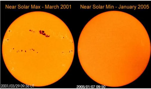
Solar maximum and solar minimum refer to epochs of maximum and minimum sunspot counts respectively. Figure 1.1 shows the visible disk of the sun near solar maximum and solar minimum.
Figure 1.1: Illustration of solar maximum and minimum periods. Very few or the absence of sunspots on the solar disc are observed near solar minimum. A large number of sunspots correspond to the period of high solar activity. [Images courtesy of SOHO; retrieved from: www.windows.ucar.edu/sun/solar variation]
The modern understanding of sunspots is that the sunspot cycle is closely related to the magnetic structure of the Sun. In 1908, the American astronomer G. E. Hale suggested a 22 year solar magnetic cycle where the sun’s dipolar magnetic field reverses each 11 years. Therefore, for modelling purposes, at least 22 year’s worth of data is required. In Chapter 2, a brief theoretical discussion about solar magnetism will be given.
1.2
Solar activity indicators
Measurements of the number of sunspots visible on the solar disc gives the com-mon index of solar activity and follows approximately an 11-year cycle. The In-ternational Sunspot Number (SSN) also known as the Wolf Number, is currently compiled and reported by the Sunspot Index Data Centre (SIDC) in Brussels, Belgium and is considered as standard. The sunspot number is also compiled by NOAA, the US National Oceanic and Atmospheric Administration.
Another indicator of the level of solar activity is the flux of radio emissions from the sun at a wavelength of 10.7 cm (2.8 GHz). This flux has been measured daily since 1947. The 10.7 cm solar flux (SF) is highly correlated with the sunspot number and is considered as a superior measure of solar activity since it can be measured objectively. However, the index is available since 1947 covering only 5 solar cycles, which limits its applicability to empirical models such as the one devel-oped in this thesis. The 10.7 cm SF has been recorded routinely by the Algonquin Radio Observatory, near Ottawa in Canada. In 1991 the program transfered to the Dominion Radio Astrophysical Observatory near Penticton, British Columbia. Fluxes are measured in units of 10−22Js−1m−2Hz−1 or solar flux units (sfu).
Geomagnetic indices also provide advance information on the amplitude of the solar activity cycle (Hathaway and Wilson, 2006). The geomagneticaa index has proved very useful for the prediction of the maxima of smoothed sunspot numbers (Kane, 1997). Details on the description and use of the geomagnetic activity aa
index for solar cycle prediction will be discussed in Chapter 3.
Another parameter characterising solar activity is the Total Solar Irradiance (TSI). This is the amount of solar radiation received at the top of the Earth’s atmosphere. A record of TSI compiled from the measurements made by five different space-based radiometers (satellites) since 1978 shows a prominent 11-year cycle with similar levels during the two recent SC minima1986 and 1996 (Frohlich, 1998). In order to improve our understanding of solar cycles, long-term and consistent measurements of the above important solar and geophysical parameters should be
1.4 CHAPTER 1. INTRODUCTION
continued and their quality maintained (Joselyn et al., 1996). For this study, the parameters with the longest recorded history, SSN and geomagneticaa index, have been used.
1.3
Space weather
Solar activity is the dynamic energy source behind all solar phenomena driving Space Weather (SW). During an active solar period, violent eruptions occur more often on the Sun. Solar flares and vast explosions known as Coronal Mass Ejections (CMEs) shoot energetic and highly charged particles towards Earth. The ensu-ing ionospheric and geomagnetic disturbances greatly affect power grids, critical military and airline communications, satellites, Global Positioning System (GPS) signals and may even threaten astronauts with harmful radiation. The same storms illuminate night skies with brilliant sheets of red and green known as aurorae or northern and southern lights (http://www.noaa.gov; http://www.sec.noaa.gov). All these phenomena are most frequent near the maximum of each 11-year cycle of solar activity. More about the way solar storms affect modern-made man gound and space based technological system can be found in various literature including Koons and Gorney (1990) and Clilverd et al.(2005).
The Maunder minimum (1645-1715) refers to a period when very few sunspots were observed. During this period, the Earth climate was cooler than normal (Kivelson and Russell, 1995). This period mimics the solar cycle climate change connections and is the subject of many studies. As indicated by Sello (2001), the particles and electromagnetic radiations flowing from solar activity outbursts are important for long term climate variations .
1.4
Predicting the solar activity cycle
In the previous section, various aspects of solar driven space weather have been discussed. In order to project space weather effects into the future, it is important to be able to project the sunspot cycle to future dates (Wilson et al., 1999). The magnetic activity on the Sun varies dramatically over time, with an almost
pe-cycle predictions, an issue which is complicated by the lack of a successful quan-titative, theoretical model of the Sun’s magnetic cycle (Joselyn et al., 1996).
Many attempts to predict the future behaviour of solar activity are well docu-mented in the literature. Hathaway et al. (1999) synthetises SC prediction tech-niques in two categories: regression techtech-niques and precursor techtech-niques. Ac-cording to this author, regression techniques use observed values of solar activity from the recent past to extrapolate into the near future. These techniques include standard regression and autoregression, curve-fitting and neural networks. The precursor techniques provide an estimate of the amplitude for the next solar cycle using mainly geomagnetic indicators.
Sello (2001) classifies solar activity prediction techniques in the following cate-gories: Precursor, Curve fitting, Spectral, Climatology and Neural Networks. The research presented in this thesis is based on Neural Network (NN) technique. A review of NN literature is presented in the following section.
1.4.1
Predicting the solar cycle using Neural Networks
NNs have been employed in solar-terrestrial modelling and prediction. Macpherson
et al. (1995) and Fessantet al. (1996) described NNs as a suitable method for SC prediction. Calvo et al.(2000) indicated that the NN computational architectures can be used advantageously to replace the standard linear statistical techniques . According to Lundstedtet al.(2005), solar activity can be described as a non-linear chaotic dynamic system and given its non-linear ability, NN should be convenient method for solar activity prediction. A version of NN known as Feed Forward Neu-ral Network (FFNN) has been used in the prediction of various solar-terrestrial time series. Conway et al. (1998) applied this technique to predict the maximum SSN for SC 23 (which occurred in 2000) with a value of 130±30. Note that the maximum SSN value of SC 23 as predicted by Conwayet al.(1998) using NNs was closer to the achieved (SSN maximum= 122) in 2000, than the prediction using precursor methods which overestimated the maximum SSN value (Hathaway and Wilson, 2006).
1.5 CHAPTER 1. INTRODUCTION
Details of the description, methodology and application of FFNN to time series prediction are given in various articles including Macpherson et al. (1995), and an introduction to the basics of NN will be given in Chapter 2
1.4.2
Solar cycle 24 prediction
Each solar cycle lasts about 11 years from one minimum to the following and is given a number, with SC 1 beginning around 1755 (Stix, 1989). The SC 23 has lasted longer than expected and currently, the minimum of SC 24 is still not well defined. On the 4 January 2008, the Solar and Heliospheric Observatory (SOHO) showed a high latitude and reversed polarity sunspot. For some experts, this solar event marked the beginning of SC 24:
(http://science.nasa.gov/headlines/y2008/10jan−solar cycle24.htm ).
However, during the last week of March 2008, sunspots with the same magnetic polarity as sunspots for SC 23 were observed. According to the NASA solar physi-cist, David Hathaway at the Marshall Space Flight Center, SC 24 has begun, but two solar cycles are simultaneously in progress until cycle 24 increases in activity. These observations indicate that the SC 24 maximum may probably not occur until 2012:
(http://science.nasa.gov/headlines/y2008/28mar−oldcycle.htm?list53494). Based on the above information, January 2008 has been considered as the start of SC 24. A number of predictions on the new cycle have been attempted. In his report of May 2007, Pesnell (2007) reports 45 predictions of SC 24 by different experts using different methods. Looking at those predictions, differences are clear both in the magnitude and timing of SC 24. While some experts forecast a much higher solar activity for SC 24 reaching a SSN maximum of 180±32, others predict a lower activity cycle with a value of 42±35 for the SSN maximum. The report shows that almost a half of the predictions agree that SC 24 will be an average cycle within the limits of the achieved SSN maximum for SC 23. Despite the apparent differences observed in the predictions, Pesnell (2007) emphasises the necessity to have quantitative estimates of the uncertainty of the predictions, which will assist in estimating the likelihood consequences of space weather in SC 24.
1.5
Objectives of the research project
The aim of this research was to develop a NN model for predicting the behaviour of SC 24. The simplicity and recent success of FFNN in forecasting solar-terrestrial phenomena explain why this method has been chosen for the SC 24 prediction. The SC 24 prediction model was developed for use in the Hermanus Magnetic Ob-servatory (HMO) Space Weather Center, the Regional Warning Center for Africa. In addition, since ionospheric behaviour is solar activity dependent (Fessantet al., 1996), any prediction of the future behaviour of the ionosphere should include an estimate of solar activity. Recently, NNs have been used to produce a reliable bottomside ionospheric model for South Africa (McKinnell, 2002), which consid-ers solar activity in terms of SSN as the main input for NN model. Therefore, the outcome of this research project will also contribute to the improvement and forecasting of the South African ionosphere.
This thesis is structured as follows:
Chapter 1 gives a general introduction to the thesis. chapter 2 discusses the basics (theories) of solar magnetism and NNs.
Chapter 3 describes the data used as input-output parameters for the NN model developed. Chapter 4 describes the development and application of the NN model for predicting the SC 24. The results and a discussion of the prediction are pre-sented in Chapter 5, while the overall conclusions comprise Chapter 6.
Chapter 2
Theoretical background
Sunspots are fascinating structures observed on the solar photosphere, the vis-ible part of the star which sustains life on our planet. In this chapter a short description of the Sun and its physical properties are given. The physics behind the sunspot equilibria is outlined using the main reduced magnetohydrodynamics (MHD) equations. Also discussed in Chapter 2 is the solar dynamo theory which is currently used to explain the solar magnetic cycle. In the second part of this chapter, the basic principles of Neural Networks as used for time series predic-tion are provided. In all cases, only the theoretical background pertaining to the research described in this thesis is provided.
2.1
Elements of solar physics
2.1.1
Physical properties of the Sun
The Sun is an ordinary star, the nearest to us and is the source of heat which sustains life on Earth and controls both terrestrial and space weather. The follow-ing are the main physical characteristics of the Sun as adapted from Kivelson and Russell (1995).
• Age = 4.5×10⁹ years
• Mass = 1.99×1030kg (330.000 times Earth’s mass)
• Mean distance from Earth (1AU = 1.5×10⁸ km (it takes sunlight 8 minutes to reach the Earth)
• Emitted Radiation (luminosity)= 3.86×1026 W (3.86×1033ergs−1)
• Equatorial rotational period = 26 days
• Effective temperature = 5785 K
The Sun is a giant mass of incandescent gas. From the interior, the Sun’s atmo-sphere consists of three layers: the photoatmo-sphere, the chromoatmo-sphere and the corona. The photosphere is the lowest and densest level of the solar atmosphere and it is the only part of the Sun that our eyes can see. However the apparent surface of the Sun is actually an illusion caused by the gas of extremely high opacity; in reality, the Sun does not have a solid surface.
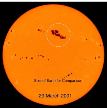
Detailed observations indicate that the photosphere is often pitted with dark spots called sunspots, the largest being much bigger than the size of the Earth (see Figure 2.1). In Europe, sunspots were discovered between 1610-1611 soon after the discovery of the telescope, but ancient Chinese records indicate that large sunspots were already seen at least 2000 years ago (Lang, 2001).
Sunspots appear dark against the brighter photosphere because they are cooler. The photosphere has a temperature of around 5500 K, while sunspots can be 1000 to 2000 k cooler. Detailed features of sunspots as revealed by modern telescopes show that a simple sunspot has a dark center, called theumbra, surrounded by a lighter penumbra. In the central umbra, the temperature is about 4100 K and the magnetic field strength can be as much as 0.3 T. The powerful magnetic fields in sunspots restrict the flow of heat into sunspot areas, keeping them cooler than the surrounding photosphere.
Sunspot structures are complicated and scientists do not fully understand the way in which they form, remain cool and then disappear. Sunspots appear and disap-pear, rising from inside the Sun and going back into it. The duration of sunspots varies from a few hours to weeks and even months. A complete understanding of sunspots requires an understanding of solar magnetism. In fact, it is well known
2.1 CHAPTER 2. THEORETICAL BACKGROUND
Figure 2.1: Large dark sunspot observed during the last solar maximum period, as compared to the size of the Earth. [Image retrieved from: www.wisc.edu/ sparke/]
.
that all solar activity is a consequence of the existence of the magnetic field on the Sun (Stix, 1989).
2.1.2
Sunspot equilibria
The Sun’s magnetic field is due to the movement of its plasma. As the solar plasma moves, any magnetic field line is pulled along with it: the magnetic field lines are frozen into the solar material. The Sun’s magnetic field can therefore exert a force on the solar plasma and create structures such as sunspots. The out-ward pressure of the strong magnetism from the Sun’s interior do not expand nor disperse because the internal gas holds the magnetic fields together, concentrating and holding them within sunspots.
The interaction of plasma and the magnetic field can be modelled using the princi-ples of magnetohydrodynamics (MHD), as summarized from Kivelson and Russell (1995):
MHD approximations provide us with two main reduced MHD equations, one for the plasma velocity u, and another for the magnetic field B. The induction equa-tion:
∂B
∂t =∇ ×(u×B) +η∇
2B (2.1)
where η= 1/(µoσ) is the magnetic diffusivity. In the above equation, the ratio of
the first term to the second term on the right is the magnetic Reynolds number:
Rm = uLη =µoσuL
which is enormous for solar phenomena (106−1012) and L is a characteristic scale length for changes of the field and flow. Thus, the magnetic field is frozen in to the plasma.
The second reduced MHD equation is the momentum equation:
ρdu
dt =−∇p+j×B+ρg (2.2)
where jis the current density; p is the plasma pressure; ρ the plasma density and
g is a constant representing the effect of gravity.
On the right hand side of the above equation, the first two terms represent the effects of the thermal pressure and of the magnetic pressure and curvature. The magnetic force can be decomposed by writing:
j ×B =−∇ B2 2µo + B· ∇ µo (2.3) in which the first term on the right represents the effect of a magnetic pressure force acting from regions of high to low magnetic pressure [pB = B
2
(2µo)]. The ratio of the plasma pressure to the magnetic pressure is conventionally represented by the symbol β where:
β= p
pB
(2.4) In solar active regions, the magnetic forces are more dominant than the thermal pressure force.
2.1 CHAPTER 2. THEORETICAL BACKGROUND
Equilibria of sunspots can be described by the force balance.
j ×B − ∇p+ρg = 0 (2.5)
Along the magnetic field, there is no contribution from the magnetic force and there exists a hydrostatic equilibrium between pressure gradients and gravity. In places like active regions, the magnetic field dominates, and the above equation reduces to:
j×B = 0 (2.6)
and the fields are said to be force-free.
As explained again in Kivelson and Russell (1995), a magnetic-flux tube below the surface tends to rise by the process of magnetic buoyancy. Lateral total pressure (plasma and magnetic) balance between the flux tube and its surrounding field-free region (p0) implies that:
p+B 2
2µ =p0 (2.7)
and so
p < po. (2.8)
For smaller temperature differences
ρ < ρ0. (2.9)
Hence, the flux tube is less dense than its surroundings and experiences an up-ward bouoyancy force. When the tube rises and breaks through the solar surface, it creates a pair of sunspots of opposite polarity as often observed (see Figure 2.2).
Figure 2.2: Magnetic ropes breaking through the solar photosphere to form sunspots, appearing in pairs of opposite polarity. This illustration which com-pare a bipolar sunspot with a polar U-shaped polar magnet was done by Randy Russell using an image from NASA’s TRACE sattelite.[Image retrieved from: http://www.windows.ucar.edu/]
.
2.1.3
The solar magnetic activity cycle and the solar
dy-namo theory
Magnetic fields in sunspots were first measured in 1908 by the American as-tronomer George Ellery Hale, who suggested a sunspot cyclic period of 22 years, covering two polar reversals of the solar magnetic dipole. The magnetic field strength in sunspots is about 0.3 T, thousands times stronger than the Earth’s magnetic field (3×10⁻⁵ T) at the equator. According to Hathaway et al. (1999) the cyclic magnetic behaviour observed through sunspots can be explained by the Sun’s differential rotation, meridional circulation, and large-scale convective mo-tions.
A qualitative model to explain the dynamics of solar magnetism and related sunspots was first proposed by Babcok (1961):
2.1 CHAPTER 2. THEORETICAL BACKGROUND
• The 22-year cycle begins with a well-established dipole field component aligned along the solar rotational axis.
• Due to the solar differential rotation (the solar rotation at the equator is 20 percent faster than at the poles), the magnetic field lines are wrapped.
• After many rotations, the field lines are highly twisted and bundled resulting in the increase of the magnetic field intensity. The resulting buoyancy lifts the bundle to the solar surface and forms a bipolar field that appears as two spots.
The above generally agreed theory does not however explain some aspects of the solar cycle such as the disappearance of sunspots for a long period. Figure 2.3 is an illustration of the Babcock model explaining the dynamics of sunspots.
Figure 2.3: Illustration of the solar magnetic activity cycle: At the start of a SC, magnetic field lines are aligned along the solar rotational axis. Due to so-lar differential rotation, field lines are wrapped and bundled in flux tubes near the Sun’s equator. The magnetic buoyancy lifts the flux tubes above the so-lar surface creating biposo-lar sunspots. [Illustration retrieved from the webpage: http://physics.uoregon.edu]
Figure 2.4: The magnetic polarity of sunspts during an 11-year solar cycle. In each hemisphere, the leading spots (in a bipolar) have the same polarity as the corresponding solar dipole magnetic field. After an almost 11-year cycle, this polarity reverses such that the complete magnetic cycle lasts 22 years. [Image retrieved from the webpage: http://physics.uoregon.edu]
During one 11-year cycle, the magnetic polarity of all the leading (westernmost) spots of the bipolar in the northen hemisphere is the same, and is opposite to that of leading spots in the southern hemisphere as shown by Figure 2.4.
The magnetic polarity of the leading spots reverses in each hemisphere at the be-ginning of the next 11-year cycle as it does the dipolar magnetic field at the solar poles. For the next 11 years in the new cycle, all polarities will be exchanged. Therefore, a full magnetic cycle on the Sun takes an average of 22 years (Lang, 2001).
The positions of sunspots and their associated active regions vary during an 11-year cycle. The first spots of each cycle appear at a latitude of about 30o
−35o in
both hemispheres. As the cycle advances, the zone of sunspot occurrence migrates towards lower latitudes, and the last spots of a cycle are normally within ±10o
of the equator. The latitude migration of sunspots is generally better represented by the famous butterfly diagram (Stix, 1989) as illustrated in Figure 2.5. More details on the basics of solar cyclic magnetism and related sunspot dynamics can be found in Kivelson and Russell (1995), Stix (1989) and Lang (2001).
2.2 CHAPTER 2. THEORETICAL BACKGROUND
Figure 2.5: The latitude migration of sunspots is commonly illustrated by the Butterfly diagram. The upper panel illustrates the latitude migration of sunspots. They form at about 30 degrees latitude at the beginning of a new cycle and migrate to the Sun’s equator as the cycle progress. The bottom panel gives the total area of the sunspots given as percentage of the visible hemisphere; [Illustration retrieved from the webpage:http://science.msfc.nasa.gov/ssl/pad/solar/images/bfly.gif].
2.2
The basics of Neural Networks
An Artificial Neural Network (ANN) is an information-processing system consist-ing of a large number of simple processconsist-ing elements calledneurons or units. ANNs simulate to some extent the structure and functioning of biological neural networks (NNs) and are characterised by (1) the pattern of connection between the neurons, (2) the method of determining the weights on the connections (training or learning algorithm) and (3) the activation function (Fausett, 1994).
In the NN models used for predictions, three types of units (neurons) are defined:
2. output units which store the output values corresponding to a given set of input values and give the results of the neural network’s processing
3. hidden units which keep the internal representation of the problem
Units in layers are connected by weights which keep the knowlege of the network and govern the influence each input has on each output. Weights are adjusted by a learning process which involves the comparison of network calculations with input-output data for known cases. The process of adjusting weights is known as
network training. During the training, weights are determined for the network to properly relate inputs to desired outputs. Hence, the network learns to predict outcomes from experience rather than from using causal laws (Macpherson et al., 1995).
2.2.1
Feed-Forward Neural Networks
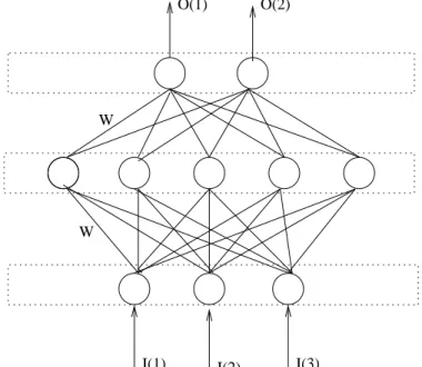
Feed Forward Neural Network (FFNN) represents the simplest and most popular type of NN, and this technique has been widely used with success in the pre-diction of various solar-terrestrial time series (Conway et al., 1998). In a FFNN arrangement, neurons (units) between layers are connected in a forward direction. Neurons in a given layer do not connect to each other and do not take inputs from subsequent layers. The input units which are set to the previous values of the time series send the signals to the hidden units. These hidden units process the received information and pass the results to the output units which produce the final response to the input signals.
2.2 CHAPTER 2. THEORETICAL BACKGROUND
Figure 2.6 is a simplified schematic of a 3-5-2 FFNN with 3 input nodes, 1 hidden layer containing 5 hidden nodes, and 2 output nodes.
Outputs Hidden Inputs W W nodes nodes nodes
I(1) I(2) I(3)
O(1) O(2)
Figure 2.6: A simplified schematic of one hidden layer FFNN. Units between layers are connected in a forward direction. Weight (W) connections between layers are adjusted during the training process.
In general, to solve a nonlinear problem with the NN technique requires (1) choos-ing a convenient network architecture, (2) selectchoos-ing a large database of input-output pairs (patterns) that contains sufficient historical information about the time series, and (3) training the network to relate the inputs to the corresponding outputs, a process by which weights are adjusted according to the back propaga-tion algorithm.
If the input neurons are external valuesAi, then the values of the hidden neurons,
Bj are set according to the equation
Bj =g I X i=1 wjiAi−φj ! , J = 1, ..., H (2.10) where w are parameters called the input weight connections, φ are the input
thresholds (also known as biases) and g(x) is the input activation function. The output neurons have their values Ck defined by:
Ck =G H X j=1 wkjBj−θk ! , k = 1, ...., O (2.11)
where G(x) is the output activation function, θk are the outputs (biases) and wkj
are the output weight connections.
One of the most typical input activation functions is the binary sigmoid function, which has a range of (0,1) and is expected to saturate ( approach the maximum and minimum values asymptotically).It is defined as (Fausett, 1994):
g(x) = 1
1 +exp(−x) (2.12)
The output activation functions can be a sigmoidal activation function as well, but sometimes it is convenient to use a linear activation functionG(x) =x.
Generally, the time series is split into two data sets: a training set and a test set. The training set is used to adjust the weights during training, while the test set is used to verify the prediction performance of the network (Fessant et al., 1996). The network is trained using past examples with the aim that the NN should have a minimal generalisation error in order to perform better on future examples. Be-fore training, both the training and testing data sets are split randomly in order to avoid the training results becoming biased towards a particular section of the database. To determine how the NN has learned the behaviour in the input-output patterns, a data set known as the validation set is used and this set consists of the data not involved in the network training process.
The training is repeated over a number of iterations until the network has at-tained the generalisation ability. The rate of the training process is controlled by a parameter known as the learning rate (a small learning rate is generally used, between 0 and 1). Overtraining can lead to NN overfitting where the NN learns the noise in the training set rather than learning to represent the system dynamics in general. This occurs when the error on the testing set starts to increase while
2.2 CHAPTER 2. THEORETICAL BACKGROUND
the training set error starts decreasing. Just before this point is reached, training is stopped because the network’s generalisation ability has reached its optimum level (Macpherson et al., 1995).
2.2.2
Back propagation of errors algorithm
There exists a number of methods available by which weights are adjusted during the training process. The most popular is the Back propagation of errors which some authors call thegeneralized delta rule. For a FFNN having I inputs,H hid-den units and O outputs (I-H-O), each training pattern consists of I inputs and
O desired outputs.
Let us denote ξµ, as the input vector and ζµ as the desired output vector whereµ
is a label for a particular training pattern. Next, an error measure must be con-structed that quantifies the accuracies of the NN’s inputs. The simplest measures the square error summed over all the outputs on training pattern µ,
Eµ= 1
2(ζ
µ
−C(w, ξµ))2
(2.13) where C(w, ξµ) is the vector composed of the NN’s outputs when presented with
input vectors ξµ. The object of training is to try to minimise Eµ for all µ. This
is done by calculating the gradient of Eµ with respect to each weight parameter.
The gradient ofE is a vector consisting of the partial derivatives ofE with respect to each of the weights. This vector gives the direction of the most rapid increase inE and the opposite direction gives the direction of most rapid decrease in error.
By differentiating the above equation with respect to an output weight connection (from equations 2.11 and 2.13), we have:
∂E ∂Wkl = ∆kBl, (2.14) where ∆k = (Ck−ζk)G′ H X j=1 WkjBj ! . (2.15)
Similarly for the input weight connections (from Eqs 2.10 and 2.13): ∂E ∂Wmn =δmξn, (2.16) where δm =g′ I X i=1 Wmiξi ! O X k=1 ∆kWkm. (2.17) If ∆Wklµ and ∆Wµ
mnrepresent the alterations to the corresponding weights after
patternµ has been presented, then they are given by the learning rules
∆wklµ =−ǫ∆µkBlµ (2.18) and ∆wµmn=−ǫδ µ mξ µ n (2.19)
whereǫ is called the learning rate and determines the step-size of each alteration.
From the preceding analysis, it can be seen that the back propagation algorithm basically consists of calculating the delta’s rule using equations 2.14 and 2.16 fol-lowed by the application of the learning rules in equations 2.18 and 2.19. FFNNs have the property of universal approximation. When given enough hidden neu-rons, they are capable of fitting any continuous function (Conway, 1998).
The above short description on the basics about FFNN and the back-propagation of errors algorithm has been compiled mainly from Conway (1998). More details can be obtained from that article and also from Fausett (1994) and Haykin (1994). The following chapter provides a detailed description of the input-output param-eters considered in order to construct the NN model for predicting solar cycle 24.
Chapter 3
The data: input-output
parameters
One of the fundamental requirements for predicting using NNs is the determination of suitable input-output parameters for the learning process. A detailed description of the parameters considered for the prediction of SC 24 is provided in this chapter.
3.1
International Sunspot Number
The relative sunspot number R introduced byR. Wolf in 1848 is the common mea-sure of solar activity. Also known as Wolf’s number or the International Sunspot Number (SSN), it is a standard daily index constructed from many measurements and the daily values are averaged monthly to remove the variations associated with the Sun’s 27-day synodic rotation period (Hathaway et al., 1999).
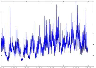
Generally the index follows an 11-year cycle, but as can be seen from Figure 3.1, the raw data exhibits complex variability in amplitude, shape and duration from cycle to cycle. These high fluctuations in sunspot number are mostly observed near solar maximum as shown by Figure 3.2. It is this extreme variability which makes the SSN one of the most difficult time series to predict (Macpherson, 1993).
18680 1888 1908 1928 1948 1968 1988 2008 50 100 150 200 250 300 Year Monthly average SSN c11 c12 c13 c14 c15 c16 c17 c18 c19 c20 c21 c22 c23 Observed SSN
Figure 3.1: Plot of the monthly average SSN against time. An 11-year cyclic period is clearly seen, but the shape and amplitude of the SCs change from one cycle to another 0 50 100 150 200 250 300 350 0 50 100 150 200 250
Day number (Year 2000)
Sunspot number
Figure 3.2: The complex fluctuations in daily sunspot number during solar maxi-mum. Plot of daily SSN during the year (2000) of solar maximaxi-mum.
3.2 CHAPTER 3. THE DATA: INPUT-OUTPUT PARAMETERS
The International SSN is currently produced by the Solar Influences Data Cen-ter (SIDC) in Brussels, Belgium and also by the U.S National Geophysical Data Center (NGDC) in Boulder, Colorado. In this study, daily, monthly average, and yearly mean SSN values were used, and all the data were obtained electronically from the SIDC website: http://sidc.oma.be
The smoothed monthly SSN is commonly used to characterise the solar cycle maximum. Both the SIDC and NGDC provide smoothed monthly SSN data. This smoothing is done in order to minimise the short-term complex variations (even on a monthly scale) observed in the raw data. The often used smoothing function is the 13-month running mean defined by Conway (1998) as,
Rismooth = 1 13 6 X j=−6 Ri−j (3.1) or Rsmooth i = 1 12 5 X j=−5 Ri−j + 1 2(Ri−6+Ri+6) ! (3.2) where i is the actual month to be smoothed, and j is the number of monthly average SSNs over which Ri is calculated before and after the month of interest.
3.2
Geomagnetic
aa
index
The geomagnetic aa index measures the global geomagnetic activity and provides one of the longest data sets which can be used in the analysis of solar terrestrial phenomena. It is therefore very useful for understanding the long-term behaviour of the Sun (Clilverd et al., 2005).
Theaa index is a three-hourly global geomagnetic activity index determined from the K-indices scaled at two antipodal sub-auroral observatories, currently Hart-land in UK, and Canberra in Australia. The three-hourly aa index is the mean of the northern and southern values, weighted to account for small differences in the latitudes of the two stations. In units of nT (nano teslas), daily values of the aa
servatory networks.
The advantage of using aa indices for research purposes is the fact that the time series spans back to 1868, further than any other planetary index. The aa data appear (in units of nT) in the Solar Geophysical Data (SGD) reports of NOAA. For this thesis, daily, monthly average as well as yearly meanaa index values were used and obtained electronically from the NGDC website:
ftp://ftp.ngdc.noaa.gov/STP/SOLAR− DATA/RELATED−INDICES
3.3
The
aa
index and solar cycle relationship
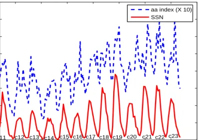
Geomagnetic indices are useful datasets which indicate solar activity levels. Solar phenomena such as solar flares and coronal mass ejections (CMEs) produce varia-tions in the solar wind that in turn cause fluctuavaria-tions in the Earth’s magnetic field (Hathawayet al., 1999). Figures 3.3 and 3.4 show a rough correlation between the 11-year solar cycle and the geomagnetic aa index.
3.3 CHAPTER 3. THE DATA: INPUT-OUTPUT PARAMETERS 18680 1888 1908 1928 1948 1968 1988 2008 10 20 30 40 50 60 Year
Monthly average aa index [nT]
Figure 3.3: This is the plot of monthly averaged geomagneticaa index from 1868. Monthlyaa index variation is complex but the minima and peaks show a roughly 11-year cyclic trend.
1880 1900 1920 1940 1960 1980 2000 2020 0 50 100 150 200 250 300 350 400 Year
Yearly mean of aa index (X10) and SSN
c11 c12 c13 c14 c15 c16 c17 c18 c19 c20 c21 c22 c23 aa index (X 10) SSN
Figure 3.4: Illustration of the modulation existing between solar activity cycle and geomagnetic aa index. Annual means of SSN and aa index values are plotted against time. In order to show clearly the 11-year modulation existing between the two indices, aa index (dotted line) values were multiplied by ten.
The geomagneticaa index is largely used for solar cycle prediction in the so called
precursor methods, which are currently the most successful and are believed to be correlated with the solar dynamo mechanism (Sello, 2001). Thompson (1993) indicated that the imminent solar cycle starts in the declining phase of the pre-vious cycle. According to Thompson (1993), in the declining phase and at solar minimum, the coming cycle is manifested by the occurrence of structures such as coronal holes and strength of the solar polar magnetic field. High speed solar wind streams from low-latitude coronal holes give rise to recurrent geomagnetic distur-bances that are used to predict the strength of the next cycle. Thompson (1993) found that the maximum amplitude of a cycle is proportional to the number of geomagnetically disturbed days (with Ap≥25) in the cycle preceding it, and this relationship is shown by equation 3.4.
On the other hand, Feynman (1982) suggested that geomagnetic activity as mea-sured by theaa index can be separated into two components:
3.3 CHAPTER 3. THE DATA: INPUT-OUTPUT PARAMETERS
• one in phase and proportional to the solar activity cycle and
• a second (residual), associated with interplanetary disturbances, which is out of phase with the solar activity cycle
The component of theaa in phase with solar activity is linked with the occurence of CMEs, while the interplanetary component of the aa index is associated with recurrent high speed solar wind streams. This component peaks mostly before solar activity minimum and is shown to be the most reliable indicator for the am-plitude of the following solar cycle maximum (Hathaway and Wilson, 2006). As it is found in the article by Hathaway et al. (1999), the solar cycle prediction methods by Feynman (1982) are indicated by the following equation:
Rmax(n) = 7.8 + 9.26aaImax(n)±13.2 (3.3)
where aaImax represents the maxima in the interplanetary component of the aa
index.
and Thompson (1993) prediction methods are represented by the equation:
Rmax(n) = 19.8 + 0.452DD(n−1)−Rmax(n−1)±16.8, (3.4)
where DD(n) is the number of geomagnetically disturbed days in cycle n, while
Rmax represents SSN maximum. Correlations in equations (3.3) and (3.4) are
r= 0.950 andr= 0.971 respectively.
Further details about Thompson’s and Feynman’s methods for solar activity pre-diction using the aa index can be found in Hathaway et al. (1999) and Hathaway and Wilson (2006). In chapter 4, a NN model developed for predicting SC 24 will be discussed. By considering the geomagneticaa index among other input param-eters, one can investigate the non-linear ability of NNs and proven superiority of the precursor techniques (Conway, 1998).
3.4
The time input parameters
The SSN temporal behavior is characterized by the parameters such as cycle min-imum date, cycle maxmin-imum date, cycle maxmin-imum amplitude, cycle rise time to maximum as well as cycle fall time to minimum. The SC properties from cycle 11-23 are shown in Table 3.1, adapted from Kivelson and Russell (1995). (Properties for SC 23 were added on the Table 3.1).
Table 3.1: Properties of SC 11-23, by (Kivelson and Russell, 1995) Cycle Start date Solar max. End date Max.SSN Length(yr) Rise(yr) Fall(yr)
11 1867.3 1870.8 1878.11 140.5 11.75 3.42 8.33 12 1878.12 1883.12 1890.2 74.6 11.25 5.00 6.25 13 1890.3 1894.1 1901.12 87.9 11.83 3.83 8.00 14 1902.1 1906.2 1913.7 64.2 11.58 4.08 7.50 15 1913.8 1917.8 1923.7 105.4 10.0 4.00 6.00 16 1923.8 1928.4 1933.8 78.1 10.08 4.67 5.42 18 1944.2 1947.5 1954.3 151.8 10.17 3.58 6.83 20 1964.10 1968.11 1976.5 110.6 11.67 4.08 7.58 21 1976.6 1979.12 1986.8 164.5 10.25 3.50 6.75 22 1986.9 1989.7 1996.8 157.6 10.00 2.85 7.20 23 1996.9 2000.4 2007.12 119.6 11.25 3.70 7.80
Assuming an approximate 11-year cycle, and considering the daily and monthly sunspot number data bases, time inputs characterising the year of a particular cycle (year index), the month number and day number in a particular year of the cycle, were defined. In order to accommodate the known periodicities and avoid discontinuities in the numerical values used to represent these time inputs, the cyclic components of month number, day number and year index were defined according to the work by Williscroft and Poole (1996) and McKinnell and Friedrich (2007), as follows: Y IS =sin 2π×Y I 11 , Y IC =cos 2π×Y I 11 (3.5) MNS =sin 2π×MN 12 , MNC=cos 2π×MN 12 (3.6) DNS =sin 2π×DN 365.25 , DNC =cos 2π×DN 365.25 (3.7) where
3.4 CHAPTER 3. THE DATA: INPUT-OUTPUT PARAMETERS
• YIS: the sine component of year index
• YIC: the cosine component of year index
• MNS: the sine component of the month number
• MNC: the cosine component of the month number
• DNS: the cosine component of the day number
• DNC: the cosine component of the day number
Hence, in addition to the geomagnetic aa index and SSN, the above defined pa-rameters were considered as time inputs for the developed NN model which is described in the following chapter.
The neural network model
For the NN to be used as a tool for prediction, input-output patterns should be constructed such that the NN training reflects the relationship existing between input and output parameters. Input parameters that are known to infuence the required output were described in the previous chapter and will be used here in developing the model. This chapter presents the development of a NN model for predicting SC 24. Three alternative methods for constructing the model and their respective NN architectures are defined and their application procedures described. For all the three alternative NN models developed, the procedure followed during the process of training is the same:
As pointed out in section 2.2.1, the data set was (before being presented to the NN) split into two independent data sets: training set and testing set. The training set contained 70% while the testing set contained 30% of the data. Data relating to SC 23 was used for the validation set.
Next, an optimal NN architecture with a good generalization ability had to be determined. As there is no generally accepted rule which guarantees the correct number of hidden nodes for a particular problem (Macpherson et al., 1995), the optimal NN had to be found experimentally by testing networks of different sizes. However, it should be noted that a certain minimum number of hidden nodes are needed to train the NN, while too many hidden nodes can lead to an overfitting of the data.
eval-4.1 CHAPTER 4. THE NEURAL NETWORK MODEL
uating the prediction accuracy over the validation data set using the root mean square error (RMSE) defined as :
RMSE = v u u t1 N N X i=1 (SSNobs−SSNpred)2, (4.1)
where N is the number of validation data set patterns, and SSNobs and SSNpred
are the observed and predicted SSN values. In the following sections, each NN model is described with its particular characteristics.
4.1
NN model 1
This model was developed based on the SSN and aa trends as observed in the historical records of the last 10 SCs. Considering Feynman’s and Thompson’s pre-diction properties using the aa index as described in Hathaway et al. (1999) and Hathaway and Wilson (2006) and outlined in the preceding chapter, a NN model was developed which operates by recognising the correlations between the geomag-netic activityaa index values of the previous cycle and the SSN of the following SC.
Therefore in the NN model developed, the geomagnetic aa index monthly val-ues were arranged with a delay of one 11-year cycle with respect to the (output) monthly SSN values. The time inputs defined in the previous chapter were ar-ranged to correspond to the monthly SSN (outputs) in the same SC. In this way, the NN makes use of them to characterize the temporal behaviour observed in the SSN historical records. The block diagram of the NN architecture illustrating the input and output to this NN model is shown in Figure 4.1.
A three layer, fully connected (see Figure 4.2) NN architecture was trained using a set of input-output pairs taken from the past history of monthly mean SSN and
aa index values. This data set covers the last 10 SCs, from SC 13-22 (SC12-21 for aa). The SSN characteristics of SC 11-23 are shown in Table 3.1 of Chapter 3. The reason for only considering 10 cycles is that SSN data for the period after 1850 are more reliable, and also correspond to data sets for which the aa index values are available.
Y I S (SC n) Y I C (SC n) M N S (SC n) M N C (SC n) aa index (SC n-1) SSN (SC n) Neural Network Model
Figure 4.1: NN architecture model 1, showing the input-output patterns. The four cyclic components of the time input in a particular SC are set corresponding to the output SSN for the same SC. Monthly values of the aa index input are those of the previous SC with respect to the output SSN.
Input layer Hidden layer Output layer . O_i I_2 I_3 I_1 I_4 I_5 H_1 H_2 H_3 H_4 H_5 W_i W_n
Figure 4.2: NN architecture showing the connections between the three layers in NN model 1. Units between the 3 layers are connected in a forward direction. Signals sent to the hidden units are assigned with weights (W) during the training process.
During the training process, the NN was presented with 1278 data points, each consisting of a pattern of 5 inputs (YIS, YIC, MNS, MNC, aa index) producing
4.2 CHAPTER 4. THE NEURAL NETWORK MODEL
one monthly SSN output. Several network sizes were tested in the search of an optimum NN architecture. As defined by equation 4.1, the FFNN architecture which had the least RMSE was taken as the optimal NN. It was obtained using 5 hidden nodes, after 1800 iterations, and a learning parameter of 0.005. The RMSE obtained from the validation data set (monthly SSN of SC 23) was found to vary between 18 and 20 with the least RMSE corresponding to 5 hidden nodes as shown in Figure 4.3. By considering this NN architecture with 5 inputs, 5 hidden nodes and 1 output (5:5:1 architecture), monthly SSN values for SC 24 were predicted taking the geomagnetic aa index values for SC 23 as inputs. The results of the prediction using this model are presented in the following chapter.
1 2 3 4 5 6 7 8 9 10 18 18.2 18.4 18.6 18.8 19 19.2 19.4 19.6 19.8 20
Number of hidden nodes
RMSE value
Figure 4.3: Optimum NN determination using the least RMSE. The RMSE scale is plotted against the changing number of hidden nodes.
4.2
NN model 2
An alternative method is to investigate the predictability of the SSN of a cycle by using the SSN of the previous SC as an input. A new NN architecture was there-fore constructed which, in contrast to the one presented in section 4.1, includes an additional input parameter which is the SSN delayed by one SC with respect to the output SSN. In fact, Thompson’s methods through equation 3.4 demonstrate the relationship between the maxima of the SSN values of a cycle and the maxima
As in NN model 1 (section 4.1), monthly SSN values for SC 13-22 and aa index values SC 12-21 were used in the training process. Each training pattern consisted of 6 inputs (YIS, YIC, MNS, MNC,aa index, SSN) producing one monthly average SSN (output). The block diagram of this NN configuration is shown in Figure 4.4 and the connections between units in layers are the same as in Figure 4.2, but in this case, there are 6 units in both the input and hidden layers.
Y I S (SC n) Y I C (SC n) M N S (SC n) M N C (SC n) SSN (SC n-1) aa index (SC n-1) SSN (SC n) Neural Network Model
Figure 4.4: NN architecture showing the input-output patterns for NN model 2. The monthly SSN delayed by one SC is also part of the input with respect to the monthly SSN (output) of the following SC
The optimum NN architecture was determined in the same way as described in Section 4.1 for NN model 1. An optimum NN architecture (with the least RMSE calculated from the validation data set) was reached using 6 hidden nodes [6:6:1 architecture], 1800 iterations and 0.005 as the learning rate. The results of the prediction using this model will also be discussed in the next chapter.
4.3
NN model 3
Based on the idea that SC 24 may present similar properties to the most recent SCs, a NN model in which the training process involves SC 21, 22 and 23 was
4.3 CHAPTER 4. THE NEURAL NETWORK MODEL
developed. The NN model was trained to predict the daily SSN of the upcoming SC using the daily values of both the aa index and the SSN of the previous cycle. Since the period involved covers only 3 SCs, the daily database (instead of the monthly database as in NN model 1 and 2) was used in order to provide the NN with sufficient information about the time series.
Hence, daily values of SSN and aa index for SC 21 were trained to predict the daily SSN for SC 22. The validation data set used was SC 23, where the daily SSN values for this SC are predicted taking the daily values of the aa index and SSN of SC 22 as inputs. The time input parameters describing the year index and the day number of the cycle (defined in Chapter 3) are also included as inputs. Hence the NN architecture consists of six inputs and one output as shown in Figure 4.5.
Y I S (SC n) Y I C (SC n) DN S (SC n) DN C (SC n) SSN (SC n-1) aaindex (SC n-1) SSN (SC n) Neural Network Model
Figure 4.5: NN architecture showing input-output patterns for NN model 3. In addition to the cyclic components of year index and day number (4 inputs), values for both the daily aa index and SSN of the previous cycle are taken as inputs for predicting the daily SSN of the following SC.
For this NN model, input-output patterns consisting of 3682 datapoints were trained. As in the previous two cases, an optimum NN architecture was deter-mined using the least RMSE calculated from the validation data set (SC 23), which was obtained expermentally by varying the number of hidden nodes. The optimum NN architecture was obtained using 6 hidden nodes [6:6:1 architecture], after 2600 iterations with a learning rate of 0.01. This optimum NN architecture was used to predict the daily SSN for SC 24, where, both daily SSN and aa index values for SC 23 were used as inputs.
A summary of the 3 NN models described in this chapter is presented in Table 4.1, and the corresponding prediction results will be discussed in the following chapter.
Table 4.1: A summary of the three NN models
Model NN architecture Inputs Iterations L.parameter Output
NN model 1 5:5:1 time inputs, 1800 0.005 Monthly SSN
aa index
NN model 2 6:6:1 time inputs, SSN 1800 0.005 Monthly SSN
+aa index
NN model 3 6:6:1 time inputs,SSN 2600 0.01 Daily SSN
Chapter 5
Results and discussion
In this chapter, prediction results obtained from the 3 alternative NN models are presented. In the discussion, the results are compared to the previously published SC 24 predictions. On the other hand, the predicted SC 23 (whose data was used as validation data set) was compared to the observed behaviour of SC 23.
5.1
The Results
5.1.1
Results of NN model 1
The NN model 1 was described in section 4.1. Its optimum NN structure was tested using the observed data of SC 23 ( validation data set). This model pre-dicts the monthly averaged SSN for SC 23 with a RMSE of 18, and a RMSE of 9 when the predicted monthly SSN are smoothed with the 13-month running mean as defined in equation 3.2. The value of the predicted smoothed monthly SSN maximum for SC 23 using NN model 1 was found to be 127±9.
Predictions for SC 24 show that the maxima in monthly sunspot number are ex-pected from late 2011 until the middle of 2013. Predictions indicate that July 2012 will be the month with the highest monthly SSN with a value of 138±18. A smoothed monthly SSN maximum for SC 24 with a value of 121±9 is predicted for June 2012. However, the smoothed monthly SSN maxima are observed from late 2011 until 2013, hence the SSN maximum could occur from at least 11 months before to 11 months after June 2012. Note that the uncertainty about the SSN
maximum for SC 24 corresponds to the RMSE calculated over SC 23 for which the NN was optimized.
The following are the main SC 24 characteristics predicted using NN model 1:
• Date of SC 24 minimum (end SC 23): January 2008 ±6 months
• Peak monthly average SSN: July 2012, with a value of 138±18
• Peak smoothed monthly SSN: June 2012, with a value of 121±9
• Date of the SC 24 maximum: June 2012± 11 months
• Date of the end of SC 24: September 2018± 6 months
The reason for considering January 2008 as the start of SC 24 was explained in section 1.4.2 of Chapter 1. A latitude of 6 months was reasonable, considering that at the time of writing (May 2008), two SCs (23 and 24) are in progress, with SC 24 expected to increase in activity. Thus the end of SC 23 and the beginning of SC 24 are yet to be defined.
5.1 CHAPTER 5. RESULTS AND DISCUSSION
Figures 5.1 and 5.2 show the predicted behavior of SC 23 and SC 24 in terms of monthly and smoothed monthly sunspot numbers respectively.
19860 1990 1994 1998 2002 2006 2010 2014 2018 50 100 150 200 250 Year Monthly averaged SSN Observed SSN Predicted SSN
Figure 5.1: The observed monthly averaged SSN values for SC 22 and 23, together with the predicted (using NN model 1) monthly averaged SSN values for SC 23 and 24.
19860 1990 1994 1998 2002 2006 2010 2014 2018 20 40 60 80 100 120 140 160 Year Smoothed monthly SSN Observed SSN Predicted SSN
Figure 5.2: The observed smoothed monthly averaged SSN values for SC 22 and 23, together with the predicted (using NN model 1) smoothed monthly averaged SSN values for SC 23 and 24.
5.1.2
Results of NN model 2
The second NN model used to predict SC 24 was described in section 4.2 of Chap-ter 4. The optimized version of this NN model predicts the monthly SSN for SC 23 with a RMSE of 23. The predicted smoothed monthly SSN maximum for SC 23 was found to be 141± 17. For SC 24, the NN model 2 predicts that the peak monthly SSN with a value of 137±23 will occur in June 2012, while the smoothed SSN maximum is expected in February 2012 with a value of 128± 17.
Figures 5.3 and 5.4 indicate the shape and amplitude of SC 23 and SC 24 in terms of monthly average and smoothed monthly SSN obtained with NN model 2.
5.1 CHAPTER 5. RESULTS AND DISCUSSION 19860 1990 1994 1998 2002 2006 2010 2014 2018 50 100 150 200 250 Year Monthly SSN Observed SSN Predicted SSN
Figure 5.3: The observed monthly averaged SSN for SC 22 and 23, together with the predicted (using NN model 2) monthly averaged SSN for SC 23 and 24.
19860 1990 1994 1998 2002 2006 2010 2014 2017 20 40 60 80 100 120 140 160 Year Smoothed monthly SSN Observed SSN Predicted SSN
Figure 5.4: The observed smoothed monthly averaged SSN for SC 22 and 23 together with the predicted (using NN model 2) smoothed monthly averaged SSN for SC 23 and 24.
5.1.3
Results of NN model 3
NN model 3 was developed to predict SC 24 using data from SCs 21, 22 and 23 and was described in section 4.3 of Chapter 4. This NN model predicts that the smoothed monthly SSN maximum for SC 24 with a value of 115±5, will occur in February 2012. Figures 5.5 and 5.6 show the predicted shape and amplitude of SC 23 and 24 in terms of monthly average and smoothed monthly SSN respectively.
19860 1990 1994 1998 2002 2006 2010 2014 2018 50 100 150 200 250 Year Monthly SSN Observed SSN Predicted SSN
Figure 5.5: Plot of the observed monthly average SSN for SC 22 and 23. The predicted (using NN model 3) monthly average SSN for SC 23 and SC 24 are shown by the dashed line.
5.1 CHAPTER 5. RESULTS AND DISCUSSION 19860 1990 1994 1998 2002 2006 2010 2014 2017 20 40 60 80 100 120 140 160 Year Smoothed monthly SSN Observed SSN Predicted SSN
Figure 5.6: The figure shows the observed smoothed monthly average SSN for SC 22 and 23. The predicted (using NN model 3) smoothed monthly average SSN for SC 23 and SC 24 are shown by the dashed line.
Figure 5.7 shows a comparison of the predictions by the three NN models and Table 5.1 summarises the predictions. In the table, predicted SC 23 and 24 maxima are given in terms of smoothed monthly SSN.
Table 5.1: A summary of the predictions from the 3 NN models Model SSN max. for SC 23 SSN maximum for SC 24 SC 24 Max. date
NN model 1 127±9 121±9 June 2012
NN model 2 141±17 128±17 February 2012
2000 2005 2010 2015 0 50 100 150 Year Yearly mean SSN 1 2 3 ob.
Figure 5.7: A comparison of SC 23 and 24 predictions using the 3 methods in terms of yearly mean SSN. The dashed line (curve 1) is the shape of SCs 23 and 24 using NN model 1. The marked solid line (curve 2) represents the prediction by NN model 2. The dotted line (curve 3) indicates the prediction by NN model 3. The thick solid line is the observed shape of SC 23 in terms of yearly mean SSN.
5.2
Discussion
To evaluate the predictions obtained using any of the 3 methods, they were com-pared to the previous predictions made for SC 23 (the observed SSN values of which were used to optimise the developed NN models). On the other hand, the predictions obtained for SC 24 were compared to those obtained and published by various groups who predicted the behavior of SC 24 using different techniques. With NN model 1 the predicted smoothed monthly SSN for SC 23 was 127±9, a value which is closer to the observed value (i.e 120 in 2000) than a consensus prediction of a much higher SC 23 maximum of 160±30 reported by Joselyn et al.
(1996). Note that the 1996 panel of experts consensus (Joselyn et al., 1996) con-sidered the precursor methods to be more accurate in SC 23 maximum prediction. However, using the NN technique, Conwayet al.(1998) predicted a SSN maximum for SC 23 with a value of 130± 30. This prediction shows an improvement with
5.2 CHAPTER 5. RESULTS AND DISCUSSION
regard to the observed SSN maximum for SC 23, and is very close to the results obtained using NN model 1.
The predicted smoothed SSN maximum for SC 23 obtained using the NN model 2 is 141± 17. This method overpredicts the observed maximum SSN in 2000, as did most of the predictions using precursor methods reported by Conway et al.
(1998) and Hathaway and Wilson (2006). However, this prediction is close to the observed maximum if compared to the consensus prediction mentioned in the pre-vious paragraph.
When tested over SC 23, NN model 3 predicts a smoothed SSN maximum value of 114± 5. Note that only the SSN maximum predicted by NN model 1 (and its uncertainty limits) is within the limits of the observed SSN maximum for SC 23. It is also important to consider that NN model 3 used the data set for only two SCs (SC 21 and 22), and therefore, despite providing the smallest RMSE (i.e 5) over the validation set, the data set used does not have sufficient information about the historical SSN and aa index behaviour.
Therefore, based on its performance on the validation data set (SC 23) and the sufficiency of database (data for 10 SCs), NN model 1 was considered as more reliable, which does not mean however that the predictions by NN models 2 and 3 have to be ruled out. In fact, the prediction results obtained from the three models predict an average SC 24 ( not very large with SSN ≥ 140 or very small with SSN≤ 100).
Note again that the smoothed SSN maximum predicted by NN model 1 within the limits of uncertainties for SC 24 includes the maxima predicted by the other two models (see Table 5.1), confirming that it should be considered as the most reliable prediction. With regard to the timing of the SSN maximum for SC 24, both models 2 and 3 (which use the SSN as input to the NN) predict the date of the SC 24 maximum for February 2012, while the NN model 1 estimates June 2012 as the date of SSN maximum. These observations indicate that the next solar maximum will most probably occur during the first half of year 2012.
The predictions obtained from NN model 1 can be placed in context by comparing them with other predictions published about SC 24.
For example, using a flux transport dynamo model and historical records of sunspot area and positions, Dikpati and Gilman (2006) predicted a much higher than av-erage cycle with a peak SSN of 150-180± 25. A large amplitude SC 24 was also predicted by Hathaway and Wilson (2006) using precursor methods by an anal-ysis of the aa index. A small SC 24 with a peak SSN of 75±8 was predicted by Svalgaardet al. (2005) using the solar dynamo polar fields observed in SC 23.
In contrast to these predictions and many others predicting very high or low values for the SSN maximum of SC 24 (summarised in Pesnell (2007)), the predictions by NN model 1 indicate an average SC 24 in agreement with a number of other predictions within the range of an average cycle shown in Table 5.2. The 10 predic-tions listed in Table 5.2 fall within the limits of the SC 24 upper and lower maxima predicted by NN model 1 as shown in Figure 5.8. The upper and lower limiting curves in Figure 5.8 are determined by the error of uncertainty which corresponds to the RMSE value calculated in the prediction of the smoothed monthly SSN for SC 23. In Table 5.3, a summary of the main cycle parameters of the predicted SC 24 is given.