Efficient strategies for deriving the subset VAR models

(1)

DOI: 10.1007/s10287-004-0021-x

Efﬁcient strategies for deriving

the subset VAR models

Cristian Gatu1and Erricos John Kontoghiorghes2,3 1 _{Institut d’informatique, Université de Neuchâtel, Switzerland.}

2 _{Department of Public and Business Administration, University of Cyprus, Cyprus.} 3 _{Computer Science and Information Systems, Birkbeck College, Univ. of London, UK.}

Abstract. Algorithms for computing the subset Vector Autoregressive (VAR) mod-els are proposed. These algorithms can be used to choose a subset of the most statistically-significant variables of a VAR model. In such cases, the selection cri-teria are based on the residual sum of squares or the estimated residual covariance matrix. The VAR model with zero coefficient restrictions is formulated as a Seem-ingly Unrelated Regressions (SUR) model. Furthermore, the SUR model is trans-formed into one of smaller size, where the exogenous matrices comprise columns of a triangular matrix. Efficient algorithms which exploit the common columns of the exogenous matrices, sparse structure of the variance-covariance of the dis-turbances and special properties of the SUR models are investigated. The main computational tool of the selection strategies is the generalized QR decomposition and its modification.

Keywords: VAR models, SUR models, Subset regression, Least squares, QR de-composition

1 Introduction

A common problem in the Vector Autoregressive (VAR) process modeling is the lag structure identiﬁcation or, equivalently, the speciﬁcation of the subset VAR models Send offprint requests to: [email protected]

_{This work is in part supported by the Swiss National Foundation for Research Grants} 101312-100757/1, 200020-10016/1 and 101412-105978.

Correspondence to: Cristian Gatu, Institut d’informatique, Université de Neuchâtel, Emile-Argand 11, Case Postale 2, CH-2007 Neuchâtel, Switzerland. e-mail: [email protected], [email protected].

CMS

Computational Management Science © Springer-Verlag 2005

(2)

[3, 7, 8, 18, 22, 27]. The vector time seriesz_t ∈ RGis a VAR process of orderp when its data generating process has the form

zt =1zt−1+2zt−2+ · · · +pzt−p+t, (1)

where_i ∈ RG×Gare the coefﬁcient matrices and_t ∈ RG is the noise vector. Given a set of realizations of the process in (1), z1, . . . , z_M and a pre-sample

z0, . . . , z1−pthe parameter matrices are estimated from the linear model

     zT 1 zT 2 ... zT M     =       zT 0 zT−1 · · · zT1−p zT 1 zT0 · · · zT2−p ... ... ... ... zT M−1zT_M−2· · · zT_M−p            T 1 T2 ... T p     +      T 1 T 2 ... T M     . (2)

In the compact form the model in (2) can be written as

Y =XB+U, (3)

whereY = (y1. . . y_G) ∈ RM×G are the response vectors, X ∈ RM×K is the lagged exogenous data matrix having full-column rank and block-Toeplitz structure,

B∈RK×G_{is the coefﬁcient matrix,}_U ₌_(u1_{. . . u}_G₎_∈_RM×G_{are the disturbances}

andK=Gp. The expectation ofUis zero, i.e. E(u_i)=0, and E(u_iuT_j)=σ_ijI_M

(i, j =1, . . . , G)[15, 17, 18, 19, 21, 25]. The VAR model (3) can be written as vec(Y )=(I_G⊗X)vec(B)+vec(U), vec(U)∼(0, ⊗I_M), (4) where vec is the vector operator and= [σij] ∈RG×Ghas full rank [6, 11]. The Ordinary and Generalized Least Squares estimators of (4) are the same and given by

ˆ

B=(XTX)−1_XT_Y.

Often zero-coefficient constraints are imposed on the VAR models. This might be due to the fact that the data generating process in (1) contains only a few non-zero coefficients. Also, over-fitting the model might yield in loss of efficiency when it is used for further testing, such as forecasting [18, 28]. A zero-restricted VAR model (ZR–VAR) is called subset VAR model. When prior knowledge about zero-coefficient constraints are not available, several subset VAR models have to be compared with respect to some specified criterion. If the purpose is the identifica-tion of a model as close as possible to the data generating process, then the use of an information criterion for evaluating the subset models is appropriate. The selec-tion criteria such as Akaike Informaselec-tion Criterion (AIC), Hannan-Quinn (HQ) and Schwarz Criterion (SC) are based on the residual sum of squares or the estimated residual covariance matrix [1, 2, 9, 23]. There is a trade-off between a good fit, i.e. small value of the residual sum of squares, and the number of non-zero coefficients. That is, there is a penalty related to the number of included non-zero coefficients.

(3)

Finding good models can be seen as an optimization problem, i.e. minimize or maximize a selection criterion over a set of sub-models derived from a ﬁnite real-ization of the process in (1) by applying a selection rule [28]. LetB=(b1. . . b_G) andS_i ∈ RK×ki _(i ₌₁_{, . . . , G)}_{denote a selection matrix such that}_β_i ₌ _ST

i bi

corresponds to the non-zero coefﬁcients ofb_i– theith column ofB. Furthermore, letX_i =XS_i which are the columns ofXthat correspond to the non-zero coef-ﬁcients ofb_i. Thus, the ZR–VAR model is equivalent to the Seemingly Unrelated Regressions (SUR) model

     y1 y2 ... yG     =      XS1 XS2 ... XSG           ST 1b1 ST 2b2 ... ST GbG     +      u1 u2 ... uG     , or

vec(Y )=(⊕G_i=₁X_i)vec({β_i}_G)+vec(U), vec(U)∼(0, ⊗I_M), (5) where ⊕G_i=₁X_i = diag(X1, . . . , X_G), {β_i}_G denotes the set {β1, . . . , β_G} and vec({β_i}_G)=(β₁T . . . β_GT)T. For notational convenience the direct sum⊕G_i₌₁and the set{·}_Gare abbreviated to⊕_i and{·}, respectively.

One possible approach to search for the optimal models is to enumerate all 2pG2 −1 possible subset VAR models. However this approach is infeasible even for modest values ofGandp. Thus, existing methods search in a smaller given subspace. One selection method is to enforce a whole coefﬁcient matrixi(1≤i≤

p), or a combination of coefﬁcient matrices to be zero. In this case, the number of the subset VAR models to be evaluated is 2p−1. Polynomial top-down and bottom-up strategies based on the deletion and, respectively, inclusion of the coefﬁcients in each equation separately have been also previously proposed [18]. Alternative methods use optimization heuristics such as Threshold Accepting [28].

Several algorithms for computing the subset VAR models are presented. The ZR–VAR model which is formulated as a SUR model, is transformed into one of smaller size, where the exogenous matrices comprise columns of a triangular matrix [6]. The common columns of the exogenous matrices and the Kronecker structure of the variance-covariance of the disturbances are exploited in order to derive efﬁcient estimation algorithms.

In the next section the numerical solution of the ZR–VAR model is given. Section 3 presents an efﬁcient variable-downdating strategy of the subset VAR model. Section 4 describes an algorithm for deriving all subset VAR models by moving efﬁciently from one model to another. Special cases which take advantage of the common-columns property of the data matrix and the Kronecker structure of the variance-covariance matrix are described in Section 5. Conclusion and future work are presented and discussed in Section 6.

(4)

2 Numerical solution of the ZR–VAR model

Orthogonal transformations can be employed to reduce to zeroM−Kobservations of the VAR model (3). This results in an equivalent transformed model with less observations, and thus, to a smaller-size estimation problem. Consider the QR decomposition (QRD) of the exogenous matrixX

¯ QTX= K R 0 K M−K, withQ¯ = K M−K ¯ QA Q¯B , (6)

whereQ¯ ∈ RM×M is orthogonal andR ∈RK×K is upper-triangular. Notice that the matrixR is a compact form of the information contained in the original data matrixX. Let ¯ QTY = G ˜ Y ˆ Y K M−Kand Q¯ T_U₌ G ˜ U ˆ U K M−K , (7) where vec(U)˜ vec(U)ˆ ∼ ⊗IK 0 0 ⊗I_M−K . Premultiplying (4) by(I_G⊗ ¯Q_A I_G⊗ ¯Q_B)T gives vec(Q¯T_AY ) vec(Q¯T_BY ) = IG⊗ ¯QTAX IG⊗ ¯QT_BX vec(B)+ vec(Q¯T_AU) vec(Q¯T_BU) .

From (6) and (7) it follows that the latter can be written as

vec(Y )˜ vec(Y )ˆ = IG⊗R 0 vec(B)+ vec(U)˜ vec(U)ˆ

which is equivalent to the reduced-size model

vec(Y )˜ =(IG⊗R)vec(B)+vec(U),˜ vec(U)˜ ∼(0, ⊗IK). (8) From the latter, it follows that (5) is equivalent to the smaller in size SUR model

vec(Y )˜ =(⊕_iR(i))vec({βi})+vec(U),˜ vec(U)˜ ∼(0, ⊗IK), (9) whereR(i)=RSi ∈RK×ki_{[5, 11, 12].}

The best linear unbiased estimator (BLUE) of the SUR model in (9) comes from the solution of the Generalized Linear Least Squares Problem (GLLSP)

argmin

V,{βi}

V2

(5)

Here = CCT, the random matrix V ∈ RK×G is deﬁned as V CT = ˜U which implies vec(V ) ∼ (0, I_GK), and · _F denotes the Frobenius norm i.e.

V2

F = Ki=1

_G

j=1Vi,j2 [15, 17, 19, 20, 21]. The upper-triangularC ∈ RG×G

is the Cholesky factor of. For the solution of (10) consider the Generalized QR Decomposition (GQRD) of the matrices⊕_iR(i)andC⊗I_K:

QT₍_⊕_i_R(i)₎₌⊕iRi 0 K∗ GK−K∗ (11a) and QT_(C_⊗_I_K_)P ₌W(0,1)W(0,2) W(0,3)_W(0,4) P =W ≡ K∗ GK−K∗ W11 W12 0 W22 K∗ GK−K∗, (11b) whereK∗ = G_i=₁k_i,⊕R_i andW are upper triangular of order K∗ andGK, respectively, andis aGK×GKpermutation matrix deﬁned as=(⊕_i(I_k_i 0)T

⊕i(0 I_K−k_i)T). Furthermore,W(0,j)(j =1,2,3,4)are block-triangular andR_i ∈ Rki×ki _{is the upper-triangular factor in the QRD of}_R(i)_{. That is,}

QT i R(i)= Ri 0 ki K−ki, with Q T i = QT Ai QT Bi ki K−ki (i =1, . . . , G), (12)

whereQ_i ∈RK×Kis orthogonal andQin (11a) is deﬁned by

Q=(⊕iQAi ⊕i QBi)=    QA1 Q_B1 ... ... QAG QBG   .

Now, sinceV2_F = PTT vec(V )2_{, the GLLSP (10) is equivalent to}

argmin

V,{βi}

PTTvec(V )2 subject to

QT_vec₍_{Y )}_˜ ₌_QT₍_⊕_i_R(i)₎_vec₍_{_β_i_}₎₊_QT_(C_⊗_I_K_{)P P}TT_vec_{(V ),}

(13) where · denotes the Euclidian norm. Using (11a) and (11b) the latter can be re-written as argmin {˜vAi},{˜vBi},{βi} G i=1 (˜vAi2_{+ ˜}_vBi2₎ subject to

(6)

vec({ ˜y_Ai}) vec({ ˜y_Bi}) = ⊕iRi 0 vec({βi})+ W11 W12 0 W22 vec({˜v_Ai}) vec({˜v_Bi}) , (14) wherey˜_Ai,v˜_Ai ∈Rki_,y˜_Bi,v˜_Bi ∈RK−ki_, ˜ yAi =QTAiy˜i, y˜Bi=QTBiy˜i (15a) and PTT vec(V )= vec({˜v_Ai}) vec({˜vBi}) K∗ GK−K∗. (15b)

From the constraint in (14) it follows that

vec({˜vBi})=W₂₂−1vec({ ˜yBi}), i=1, . . . , G (16) and the GLLSP is reduced to

argmin {˜vAi},{βi} G i=1 ˜vAi2 subject to

vec({˜˜y_i})=(⊕_iR_i)vec({β_i})+W11vec({˜v_Ai}), (17) where

vec({˜˜y_i})=vec({ ˜y_Ai})−W12vec({˜v_Bi}). (18) The solution of (17), and thus, the BLUE of (9), is obtained by settingv˜_Ai = 0 (i=1, . . . , G) and solving the linear system

(⊕iRi)vec({ ˆβ_i})=vec({˜˜y_i}), or, equivalently, by solving the set of triangular systems

Riβˆi = ˜˜yi, i=1, . . . , G. 3 Variable-downdating of the ZR–VAR model

Consider the re-estimation of the SUR model (9) when new zero constraints are imposed to the coefﬁcientsβ_i(i=1, . . . , G). That is, after estimating (9) the new SUR model to be estimated is given by

(7)

whereR˜(i) =R(i)S˜_i,β˜_i = ˜S_iTβ_i andS˜_i ∈Rki×˜ki _{is a selection matrix (0}_{≤ ˜}_k_i _≤

ki). This is equivalent to solving the GLLSP argmin

V,{ ˜βi}

V2

F subject to vec(Y )˜ =(⊕iR˜(i))vec({ ˜β_i})+vec(V CT). (20) From (11) and (15) it follows that (20) can be written as

argmin {˜vAi},{˜vBi},{ ˜βi} G i=1 (˜vAi2+ ˜vBi2) subject to vec({ ˜y_Ai}) vec({ ˜yBi}) = ⊕iRiS˜i 0 vec({ ˜βi})+ W11W12 0 W22 vec({˜v_Ai}) vec({˜vBi}) .

Using (16) and (18) the latter becomes argmin

{˜vAi},{ ˜βi}

vec({˜v_Ai})2 subject to

vec({˜˜y_i})=(⊕_iR_iS˜_i)vec({ ˜β_i})+W11vec({˜v_Ai}). (21) Now, consider the GQRD of the matrices⊕_iR_iS˜_i andW11, that is

˜ QT(⊕iRiS˜i)= ⊕iRi˜ 0 ˜ K∗ K∗_{− ˜}_K∗ (22a) and ˜ QT_W11_˜_P_˜_{= ˜}_W ₌ K˜∗ K∗− ˜K∗ ˜ W11 W12˜ 0 W22˜ ˜ K∗ K∗_{− ˜}_K∗ , (22b) whereK˜∗ = G_i=₁k˜_i,⊕_iR˜_i andW˜ are upper triangular of order K˜∗ andK∗, respectively, and˜ =(⊕_i(I_k_˜

i 0)T⊕i(0 Iki−˜ki)T). Notice that, the upper-triangular

˜

Ri ∈Rk˜i×˜ki _{comes from the QRD}

˜ QT i RiS˜i = _˜ Ri 0 ˜ ki ki−˜ki, with ˜ QT i = _˜ QT Ai ˜ QT Bi ˜ ki ki−˜ki (i=1, . . . , G), (23)

whereQ˜_i ∈Rki×ki _{is orthogonal. The latter factorization is a re-triangularization}

of a triangular factor after deleting columns [10, 11, 14, 29]. Furthermore,Q˜ in (22) is deﬁned byQ˜ =(⊕_iQAi˜ ⊕_iQBi)˜ . Ify˜_Ai∗ = ˜QT_Aiy˜˜_i,y˜_Bi∗ = ˜QT_Biy˜˜_i,

˜ PT˜T vec({˜vAi})= vec({˜v∗_Ai}) vec({˜v∗_Bi}) _˜ K∗ K∗_{− ˜}_K∗

(8)

and

vec({ ˜y_i∗})=vec({ ˜y_Ai∗ })− ˜W12vec({˜v_Bi∗ }), then the solution of the GLLSP (21) is obtained by solving

(⊕iRi˜ )vec({ ˆ˜β_i})=vec({ ˜y_i∗}),

orRi˜ βˆ˜_i = ˜y_i∗(i =1, . . . , G). Notice that, the GQRD (22) is the most expensive computation required for deriving the BLUE of the SUR model (19) after the factorization (11) has been computed.

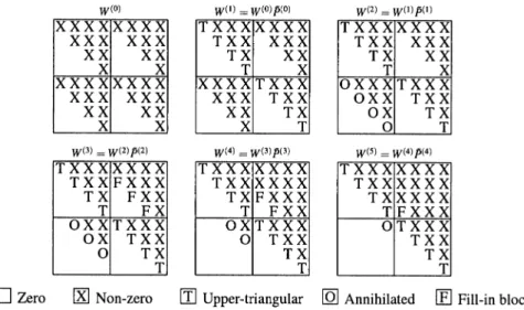
An efﬁcient strategy for computing the orthogonal factorization (22b) has been proposed within the context of updating SUR models [13]. Notice thatQ˜TW11˜ in (22b) can be written as ˜ QTW11˜ =W(0)₌ K˜∗ K∗− ˜K∗ W(0,1) _W(0,2) W(0,3) _W(0,4) ˜ K∗ K∗_{− ˜}_K∗ , (24) whereW(0,i)(i =1, . . . ,4)has a block-triangular structure. That is,W(0)has the structural form W(0)₌                 ˜ k1 k˜2 ... k˜G k1−˜k1 k2−˜k2 ... kG−˜kG W(0,1) 11 W( 0,1) 12 . . . W( 0,1) 1G W (0,2) 11 W( 0,2) 12 . . . W( 0,2) 1G 0 W₂₂(0,1). . . W₂(_G0,1) 0 W₂₂(0,2). . . W₂(0_G,2) ... ... ... ... ... ... ... ... 0 0 . . . W_GG(0,1) 0 0 . . . W_GG(0,2) W(0,3) 11 W( 0,3) 12 . . . W( 0,3) 1_G W( 0,4) 11 W( 0,4) 12 . . . W( 0,4) 1_G 0 W₂₂(0,3). . . W₁(_G0,3) 0 W₂₂(0,4). . . W₁(0_G,4) ... ... ... ... ... ... ... ... 0 0 . . . W_GG(0,3) 0 0 . . . W_GG(0,4)                 ˜ k1 ˜ k2 ... ˜ kG k1−˜k1 k2−˜k2 ... kG−˜kG . (25)

The orthogonal matrixP˜in (22b) computes the RQ decomposition of (25) using a sequence of(G+1)orthogonal factorizations. That is,P˜ = ˜P(0)P˜(1). . .P˜(G), where P˜(i) ∈ RK∗×K∗ (i = 0, . . . , G) is orthogonal. Initially, P˜(0) tri-angularizes the blocks of the main block-diagonal of W(0). I.e. P˜(0) = diag(P˜₁₁(0), . . . ,P˜₁(_G0),P˜₄₁(0), . . . ,P˜₄(_G0)), where the RQ decomposition of W_jj(0,i) is given byW_jj(1,i) =W_jj(0,i)P˜_ij(0)(i=1,4 andj =1, . . . , G). Here,W_jj(1,i)is trian-gular. The matrix

W(0)_P˜(0)₌_W(1)_≡

W(1,1)_W(1,2) W(1,3)_W(1,4)

(9)

Fig. 1.Re-triangularization ofW(0)in (25)

has the same structure as in (25), but withW(1,1) and W(1,4) being triangular. The transformationW(i+1)=W(i)P˜(i)annihilates theith super block-diagonal of

W(i,3)_{, i.e. the block}_W(i,3)

j,j+i−1(j=1, . . . , G−i+1), and preserves the triangular

structure ofW(1,1)andW(1,4). Speciﬁcally,P˜(i)is deﬁned by

˜ P(i)=                 IJi 0 · · · 0 0 · · · 0 0 0 P˜₁(i,1)· · · 0 P˜₁(i,2)· · · 0 0 ... ... ... ... ... ... ... ...

0 0 · · · ˜P_G−i+(i,1) ₁ 0 · · · ˜P_G−i+(i,2) ₁ 0 0 P˜₁(i,3)· · · 0 P˜₁(i,4)· · · 0 0

... ... ... ... ... ... ... ...

0 0 · · · ˜P_G−i+(i,3) ₁ 0 · · · ˜P_G−i+(i,4) ₁ 0

0 0 · · · 0 0 · · · 0 Iρ_i                 ,

whereJ_i = i−_j=1₁k˜_i andρ_i = i−_j=1₁(k_i − ˜k_i). Figure 1 shows the process of re-triangularizingW(0), whereG=4.

Letk1˜ =. . . = ˜k_G ≡ K/2. The complexities of computing the GQRD (22) using this variable-downdating method and that which does not exploit the structure of the matrices are given, respectively, by:

GK2₈_G2_(K₊₁₎₊_G(₃₁_K₊₁₂₎₊₇₍₁₅_K₊₄₎_/₂₄_≈_O(G3_K3_/₃_),

and

(10)

Thus, the proposed variable-downdating method is approximately 22 times faster. The number of ﬂops required for the estimation of all subset VAR models using a simple enumeration strategy is ofO((G3K3/3)2GK).

4 Deriving the subset VAR models

All possible subset VAR models can be generated by moving from one model to another. Consider deleting only theµth variable fromjth block of the reduced ZR–VAR model (9). This is equivalent to the SUR model in (19), whereS˜_j =

(e1. . . eµ−1eµ+1. . . ek_j),el is thelth column of the identity matrixIk_j,S˜i =Ik_i,

˜

βi =βi,ki˜ =ki, fori = 1, . . . , Gandi = j. Thus, the ZR–VAR model to be estimated is equivalent to the SUR model

         ˜ y1 ... ˜ yj ... ˜ yG          =          R(1) ... R(j)_Sj˜ ... R(G)                   β1 ... ˜ ST jβj ... βG          +          ˜ u1 ... ˜ uj ... ˜ uG          . (26)

The BLUE of (26) comes from the solution of the GLLSP in (21). Now, letW11be partitioned as W11 =              k1 k2 · · · kj · · · kG 1,1 1,2 · · · 1,j · · · 1,G 0 2_,2 · · · 2,j · · · 2,G ... ... ... ... ... ... 0 0 · · · _j,j · · · _j,G ... ... ... ... ... ... 0 0 · · · 0 · · · _G,G              k1 k2 ... kj ... kG .

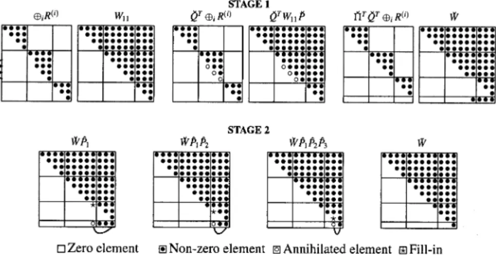
The computation of the GQRD (22) can be efﬁciently derived in two stages. The ﬁrst stage, initially computes the QRD

ˇ

QT_R_˜(j)₌Rj˜

0

and the productQˇT( j,j· · · j,G)=( ∗_j,j· · · ∗_j,G). Then, it computes the RQD

∗

(11)

Fig. 2.The two stages of estimating a ZR–VAR model after deleting one variable

orthogonalQˇT andPˇ are the products ofki −µleft and right Givens rotations which re-triangularizeR˜(j)and _j,j∗ , respectively. Furthermore, let

ˇ T ₌    I_K∗ j−10 0 0 0I_K∗ G−K∗j 0 1 0   , with K_j∗= j i=1 ki.

Thus, in (22a)Q˜T = ˇTQˇT_∗ and

˜ QT ⊕i(RiSi˜)= ⊕iR˜i 0 _˜ K∗ 1 , whereQˇT_∗ =diag(I_K∗ j−1,Qˇ T_{, I}_K_∗_−K_∗ j)andK∗≡KG∗.

The second stage computes the RQDW˜ = (ˇTW)ˇ Pˆ, where W˜ andWˇ are upper-triangular,Wˇ = ˇQT_∗W11Pˇ_∗,Pˇ_∗ = diag(I_K∗

j−1,P , Iˇ K∗−Kj∗)andPˆ is the

product of(K∗−K_j∗)Givens rotations. Theρth rotation (ρ=1, . . . , K∗−K_j∗), sayPˆ_ρ, annihilates the(K_j∗+ρ−1)th element of the last row ofˇTWˇ by rotating adjacent planes. Figure 2 illustrates the computation of the two stages, whereG=3,

k1=4,k2=5,k3=3,j =2 andµ=2. Notice that in (22b),˜ is the identity matrix andP˜ ≡ ˇP∗.

Now, letV = [v1, v2, . . . , vn]denote the set ofn = |V|indices of the se-lected columns (variables) included in the sub-matricesR(i)(i =1, . . . , G). The sub-models corresponding to the sub-sets[v1],[v1, v2],· · ·,[v1, v2, . . . , vn]are immediately available. A function Drop will be used to derive the remaining sub-models [8]. This function downdates the ZR–VAR by one variable. That is,

(12)

An efﬁcient algorithm, called Dropping Columns Algorithm (DCA) has been previously introduced within the context of generating all subset models of the ordinary and general linear models [4, 8, 24]. The DCA generates a regression tree. It moves from one node to another by applying a Drop operation, that is, by deleting a single variable. A formal and detailed description of the regression tree which generates all subset models can be found in [8]. Here the basic concepts using a more convenient notation are introduced.

LetV denote the set of indices and 0 ≤ γ < |V|. A node of the regression tree is a tuple(V, γ ), whereγ indicates that the children of this node will include the ﬁrstγ variables. IfV = [v1, v2, . . . , v_n], then the regression treeT (V, γ )is a

(n−1)–tree having as root the node(V, γ ), whereγ =0, . . . , n−1. The children are deﬁned by the tuples(Drop(V, i), i−1)fori=γ+1, . . . , n−1. Formally this can be expressed recursively as

T (V, γ )=    (V, γ ) if γ =n−1, (V, γ ), T (Drop(V, γ +1), γ ),· · · · · ·, T (Drop(V, n−1), n−2) if γ < n−2. The number of nodes in the sub-treeT (Drop(V, i), i−1)is given byδ_i =2n−i−1 andδ_i =2δ_i₊1, wherei=1, . . . , n−1 [8].

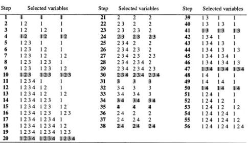
Computing all possible subset regressions of a model havingn variables is equivalent to generatingT (V,0), whereV = [1,2, . . . , n]. Generally, the com-plexity –in terms of ﬂops– of generating T (V, γ ) in the General Linear model case is ofO((|V| +γ )2|V|−γ). Thus the complexity of generating all subset VAR models using the DCA is ofO((GK)2GK). Figure 3 showsT (V, γ )together with the sub-models generated from each node, whereV = [1,2,3,4,5]andγ =0. A sub-model is denoted by a sequence of numerals which correspond to the indices of variables.

The DCA will generate all the subset VAR models by deleting one variable from the upper-triangular regressors of the reduced-size model (8). It avoids estimating each ZR–VAR model afresh, i.e. it derives efﬁciently the estimation of one ZR– VAR model from another after deleting a single variable. Algorithm 1 summarizes this procedure.

Algorithm 1Generating the regression treeT (V, γ )given the root node(V, γ ).

1: procedureSubTree(V, γ)

2: From(V, γ )obtain the the sub–models(v1· · ·vγ+1), . . . , (v1· · ·v|V|)

3: fori=γ+1, . . . ,|V| −1do

4: V(i)←Drop(V, i) 5: SubTree(V(i), i−1) 6: end for

(13)

Fig. 3.The regression treeT (V, γ ), whereV = [1,2,3,4,5]andγ =0 5 Special cases

The method of generating all subset VAR models becomes rapidly infeasible when the dimensions of the generating process (1), i.e.Gand p increase. Thus, two approaches can be envisaged. The ﬁrst is to compare models from a smaller given search space. The second is the use of heuristic optimization techniques [28]. Here, the former approach is considered.

A simpliﬁed approach is to consider a block-version of Algorithm 1, i.e. a ZR– VAR model is derived by deleting a block rather than a single variable. Within this context, in Figure 3 the numerals will represent indices of blocks of variables. This approach will generate 2G−1 subset VAR models and can be implemented using fast block-downdating algorithms [11]. Notice that the deletion of the entirejth block is equivalent in deleting thejth row from all1, . . . , _p. This is different than the method in [18, pp. 180] where a whole coefﬁcient matrix_i(i=1, . . . , p) is deleted at one time.

5.1 Deleting identical variables

Deleting the same variables from all the Gblocks of the ZR–VAR model cor-responds to deletion of whole columns from some of the coefﬁcient matrices

(14)

fori=1, . . . , Gand 0≤ ˜k < K. Thus, (9) can be written as    ˜ y1 ... ˜ yG   =    RS ... RS       ST_b1 ... ST_bG   +    ˜ u1 ... ˜ uG   . (27)

The estimation of (27) comes from the solution of GLLSP (10), where now,R(i)=

RS,β_i =STb_i andk_i = ˜kfori=1, . . . , G. The orthogonal matrices in (12) are identical, i.e.QT_i = ˇQT fori=1, . . . , Gand have the structure

ˇ QT = ˇ QT A ˇ QT B ˜ k K−˜k .

Multiplying respectively,QT andQfrom the left and right of(C⊗I_K)it results

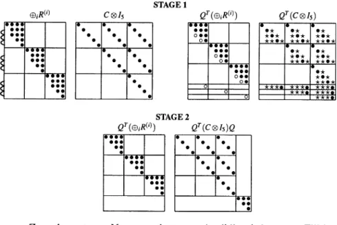
QT(C⊗IK)Q= C⊗WA C⊗WB (⊕iQAˇ ⊕iQB)ˇ = C⊗Ik˜ 0 0 C⊗I_K−˜_k .

The latter is upper-triangular. Figure 4 shows the computation ofQT(C⊗IK)Q, whereG = 3,K = 5 andk˜ = K−1. In this case, the permutation matrix in (11) is not required, i.e. =IKG and the matrixP ≡Q. Notice that for the construction ofQin (11) only aK×Korthogonal matrixQˇneeds to be computed rather than theK×KmatricesQ1, . . . , QG.

The DCA can be modiﬁed to generate the subset VAR models derived by deleting identical variables from each block. Given a node(V, γ ), the setV de-notes the indices of the non-deleted (selected) variables. The parameterγ has the same deﬁnition as in section 4. The model (27) is estimated. This provides

G|V| −γ sub-leading VAR models. Then, one variable is deleted, speciﬁcally

V(i) _{≡ [}_{v1, . . . , v}_i₋_{1, v}_i+_{1, . . . , v}_|V_|_]_for _i ₌ _γ ₊₁_{, . . . ,}_|_V_|_{. The procedure is}

recursively repeated forV(γ+1), . . . , V(|V|).

This method is summarized by Algorithm 2 which generates a regression tree of 2K −1 nodes. Each node corresponds to one of the possible combination of selecting variables out of K. In general, the regression tree with the root node

(V, γ )has 2|V|−γ−1 nodes and provides 2|V|−γ−1(|V| +γ+2)−1 subset VAR models. Figure 5 shows the regression tree for the caseK =4 andG=2. Each node shows(V, γ )and the indices of the corresponding subset VAR model in (27) together with its sub-leading models.

Notice that Algorithm 2 generates all the subset VAR models by deleting the same variables from each block when initiallyV ≡ [1, . . . , K]andγ =0. Com-pared to the standard variable-deleting strategy of Algorithm 1, it requiresO(G) less computational complexity in order to generate(K +2)2K−1−1 out of the 2KG−1 possible subset VAR models.

(15)

Fig. 4.The two stages of estimating a SUR model after deleting the same variable from each block

Algorithm 2Generating the subset VAR models by Deleting Identical Variables (DIV).

1: procedureSubTree_DIV(V, γ)

2: Let the selection matrixS≡ [ev₁· · ·ev_|_V_|]

3: Estimate the subset VAR model vec(Y )˜ =(IK⊗RS)vec({STbi})+vec(U)˜ 4: fori=γ+1, . . . ,|V|do

5: V(i)≡ [v1, . . . , vi−1, vi+1, . . . , v|V|]

6: if(|V(i)|>0)thenSubTree_DIV(V(i), i−1)end if

7: end for

8: end procedure

5.2 Deleting subsets of variables

The computational burden is reduced when subsets of variables are deleted from the blocks of the ZR–VAR model (9). Consider the case of proper subsets and speciﬁcally when Si = ki+1 ki−ki+1 Si+1 S∗_i , i=1, . . . , G−1. (28) From the QRD ofR(1) QT1R( 1)₌ R1 0 k1 K−k1 , (29)

(16)

Fig. 5.The regression treeT (V, γ ), whereV = [1,2,3,4],K=2,G=2 andγ =0

it follows that the QRD ofR(i)can be written as

QT1R(i)= Ri 0 with QT1 = QT Ai QT Bi ki K−ki, i=1, . . . , G, (30)

whereR_i is the leading triangulark_i×k_i sub-matrix ofR1. Now, the GLLSP (10) can be written as

argmin

V,{βi}

QT vec(V ) subject to

QTvec(Y )=QT ⊕_i(R(i)βi)+QT(C⊗IK)QQTvec(V ), (31) where QT = (⊕_iQT_Ai ⊕_i QT_Bi). The latter is equivalent to (14), but with

˜

vAi=QTAivi,v˜_Bi=QT_Biv_i. Furthermore, the triangularW_pq(p, q=1,2) can be partitioned as W11=           c11Ik1 c12Ik2 0 · · · c1GIkG 0 0 c22Ik2 · · · c2GIk_G 0 .. . ... ... ... 0 0 · · · cGGIk_G           , W12=           0 0 0 c12Ik1−k2 0 · · · _c 0 0 1GIk1−kG 0 0 0 · · · 0 0 c2GIk2−kG 0 .. . ... ... ... 0 0 · · · 0           , W21=0 and W22=      

c11IK−k1 0c12IK−k1 · · · 0c1GIK−k1

0 c22IK−k2 · · · 0c2GIK−k2 .. . ... ... ... 0 0 · · · cGGIK−k_G      .

(17)

This simpliﬁes the computation of the estimation of the ZR–VAR model (9) [15, 16]. Expression (16) becomes ˜ vBi =(y˜Bi− G j=i+1 cij(0 IK−ki)v˜Bj)/cii, (i=G, . . . ,1) (32a)

and the estimationβˆ_i(i=1, . . . , G) is computed by solving the triangular system

Riβˆi =y˜Ai− G j=i+1 cij 0 0 Iki−kj 0 ˜ vBj. (32b)

The proper subsets VAR models are generated by enumerating all the possible selection matrices in (28) and estimating the corresponding models using (32). This enumeration can be obtained by considering all the possibilities of deleting variables on the ﬁrst block, i.e. generatingS1and then constructing the remaining selection matricesS2, . . . , S_Gconformly with (28).

This method is summarized by Algorithm 3 and consists of two procedures. The first, SubTreeM, is the modified SubTree procedure of Algorithm 1. It gener-ates the regression tree as shown in Figure 3. In addition, for each node(V, γ ), the ProperSubsets procedure is executed. The latter performs no factorization, but computes the estimated coefficients using (32). Specifically, it derives all possible proper subsets (S1, . . . , SG) in (28), for S1 = [ev1, . . . , evγ+1], . . . , [ev1, . . . , evγ+1, . . . , ev|V|]. The ProperSubsets procedure is based on a

backtrack-ing scheme. That is, givenS1, . . . , Si−1(i =1, . . . , G), it generates a newSi and

incrementsi. If this is not possible, then it performs a backtracking step, i.e. it decrementsiand repeats the procedure. As shown in the Appendix, the number of proper subsets VAR models generated by Algorithm 3 is given by

f (K, G)= 2K−1 if G=1; min(K,G−1) i=1 Ci− 1 G−2CKi 2K−i if G≥2, whereC_nk =n!/(k!(n−k)!).

The order of generating the models is illustrated in Figure 6 for the caseK=4 andG=3. The highlighted models are the common models which are generated when the proper subsets are in increasing order, i.e.

Si+1=

ki ki+1−ki

Si S_i+∗ 1

, i =2, . . . , G.

In this case the ZR–VAR model is permuted so that (28) holds, and thus, Algorithm 3 can be employed.

The computational burden of the ProperSubsets procedure can be further re-duced by utilizing previous computations. Assume the proper subsets VAR model

(18)

Algorithm 3Generating the subset VAR models by deleting proper subsets of variables.

1: procedureSubTreeM(V, γ)

2: Compute the QRD (29) forS1= [ev1, . . . , ev|V|]

3: ProperSubsets(V, γ) 4: fori=γ+1, . . . ,|V| −1do 5: V(i)←Drop(V, i) 6: SubTreeM(V(i), i−1) 7: end for 8: end procedure 1: procedureProperSubsets(V, γ) 2: LetS1← [ev1, . . . , evγ]; k1←γ; i←1 3: while(i≥1)do

4: if(i=1andk1<|V|)or(i >1andki< ki−1)then

5: ki←ki+1; Si(ki)←ev_ki 6: if(i=G)then

7: ExtractR1, . . . RGin (30) fromR1in (29) corresponding to (S1, . . . SG)

8: Solve the GLLSP (31) using (32)

9: else 10: i←i+1; ki←0 11: end if 12: else 13: i←i−1 14: end if 15: end while 16: end procedure

corresponding to(S1, . . . , S_G−1, S_G)has been estimated. Consider now the es-timation of the proper subsets VAR model corresponding to(S1, . . . , SG−1,SG)˜ , whereSG˜ =(SG ev_kG₊₁). For example, in Figure 6, this is the case when moving from step 15 to step 16. Lety˜_BG = (ψBG y˜˜BG)T andv˜BG = (υBG v˜∗_BG)T,

wherey˜˜_BG,v˜_BG∗ ∈ RK−˜kG _and_k˜_G ₌ _k_G₊_{1. That is}_ψ_BG_and_υ_BG_{are the ﬁrst}

elements ofy˜_BGandv˜_BG, respectively. Notice that fromk˜_G=k_G+1, it implies thatK−ki < K−kGfori=1, . . . , G−1. Thus, in (32a),υBGcorresponds to a

zero entry and therefore,

˜

vBi=(yBi˜ −

G−1 j=i+1

cij(0IK−ki)vBj˜ −ciG(0IK−ki)v˜BG∗ )/ciifor i=G−1, . . . ,1.

The recursive updating formulae (32a) become

˜˜

vBG= ˜˜y_BG/cGG≡ ˜vBG∗ and vBi˜˜ = ˜vBi for i=G−1, . . . ,1.

Now, ˜˜ y_i = ˜yAi− G−1 j=i+1 cij 0 0 Ik_i−kj 0 ˜ vBj−ciG 0 0 Ik_i−kG−10 ˜ v∗_BG

(19)

Fig. 6.The sequence of proper subset models generated by Algorithm 3, forG=3 andK=4

= ˜yi+(ciGυBG)ekG+1,

wherey˜_i = R_iβˆ_i, i.e. the righthand-side of (32b). The estimation of the proper subsets VAR model comes from the solution of the triangular systems

˜ RGβˆ_G∗ = ˜ yAG ψBG and Riβˆ_i∗= ˜˜y_i, for i=G−1, . . . ,1.

The computational cost of the QRDs (12) is also reduced in the general subsets case whereS1 ⊆ S2 ⊆ · · · ⊆ SG. The QRD ofR(i) =RSi is equivalent to re-triangularizing the smaller in size matrixRi₊1after deleting columns. Notice that RSi =RSi+1S_i+T 1Siand

QT_i+1RSi =QTi+1RSi+1Si+T 1Si = Ri+1 0 S_i+T 1Si = Ri+1S_i∗ 0 .

HereS_i∗=S_i+T ₁S_i is of orderk_i+1×ki and selects the subset ofSi+1and in turn

the selected columns fromR_i+1. Now, computing the QRD

ˆ QT_i (Ri+1S_i∗)= Ri 0 ki ki+1−ki (33)

(20)

it follows that the orthogonalQT_i of the QRD (12) is given byQT_i = ˇQT_i QT_i+₁, where ˇ QT_i = ˆ QT i 0 0 I_K−k_i₊1 .

Thus, following the initial QRD ofR(G)=RS_G, the remaining QRDs ofR(i)are computed by (33) fori=G−1, . . . ,1.

Consider the case whereSG ⊆ · · · ⊆S2⊆S1. Computations are simpliﬁed if the GLLSP (10) is expressed as

argmin

V,{βi}

V2

F subject to vec(Y )˜ =(⊕iL(i))vec({βi})+vec(V CT), (34) whereL(i)=LSiand now,LandCare lower triangular [15]. Thus, instead of (6), the QL decomposition ofXneeds to be computed:

¯ QTX= 0 L M−K K , with ¯ QT(Y U)= ˆ Y Uˆ ˜ Y U˜ M−K K .

Furthermore, the QL decomposition

QT_i L(i+1)₌ 0 Li+1 K−ki ki

can be seen as the re-triangularization ofL_iafter deleting columns [14]. IfS_i₊1is a

proper subset ofS_i, i.e.S_i =(S_i∗ S_i₊1), thenL_i+1is the trailing lowerki+1×ki+1

sub-matrix ofL_i [15]. Notice that if (9) rather than (34) is used, thenR_i+1derives

from the more computational expensive (updating) QRD

QT_i+1 Ri1 Ri2 = Ri+1 0 , where Ri = ki−ki+1 ki+1 R∗ i Ri1 0 R_i2 ki−ki+1 ki+1 .

(21)

6 Conclusion and future work

Efficient numerical and computational strategies for deriving the subset VAR mod-els have been proposed. The VAR model with zero-coefficient restriction, i.e. ZR– VAR model, has been formulated as a SUR model. Initially, the QR decomposition is employed to reduce to zeroM−Kobservations of the VAR, and consequently, ZR–VAR model. The numerical estimation of the ZR–VAR model has been derived. Within this context an efficient variable-downdating strategy has been presented. The main computational tool of the estimation procedures is the Generalized QR decomposition. During the proposed selection procedures only the quantities re-quired by the the selection criteria, i.e. the residual sum of squares or the estimated residual covariance matrix, should be computed. The explicit computation of the estimated coefficients is performed only for the final selected models.

An algorithm which generates all subset VAR models by efﬁciently moving from one model to another has been described. The algorithm generates a regression tree and avoids estimating each ZR–VAR model afresh. However, this strategy is computational infeasible even for modest size VAR models due to the exponential number(2pG2 −1)of sub-models that derives. An alternative block-version of the algorithm generates(2G−1)sub-models. At each step of the block-strategy a whole block of observations is deleted from the VAR model. The deletion of theith block is equivalent in deleting theith row from each coefﬁcient matrix1, . . . , _p in (1).

Two special cases of subset VAR models which are derived by taking advantage of the common-columns property of the data matrix and the Kronecker structure of the variance-covariance matrix have been presented. Both of them requireO(G) less computational complexity than generating the models afresh. The first special case derives(pG+2)2(pG−1)−1 subset VAR models by deleting the same variable from each block of the reduced ZR–VAR model. The second case is based on deleting subsets of variables from each block of the regressors in the ZR–VAR model (10).An algorithm that derives all proper subsets models given the initialVAR model has been designed. This algorithm generatesmin_i₌₁(K,G−1)C_G−i−1₂C_Ki 2K−i models, whenGis greater than one. In both cases the computational burden of deriving the generalized QR decomposition (11), and thus, estimating the sub-models, is significantly reduced. In the former case only a single column-downdating of a triangular matrix is required. This is done efficiently using Givens rotations. The second case performs no factorizations, but efficiently computes the coefficients using (32).

The new algorithms allow the investigation of more subset VAR models when trying to identify the lag structure of the process in (1). The implementation and application of the proposed algorithms need to be pursued. These methods are based on a regression tree structure. This suggest that a branch and bound strategy which derives the best models without generating the whole regression tree should

(22)

be considered [7]. Within this context the use of parallel computing to allow the tackling of large scale models merits investigation.

The permutations of the exogenous matricesX1, . . . , X_Gin the SUR model (5) can provideG!new subset VAR models. If the ZR–VAR model (9) has been already estimated, then the computational cost of estimating these new subset models will be significantly lower since the exogenous matricesX1, . . . , XGhave been already factorized (i=1, . . . , G). Furthermore, the efficient computation of the RQ fac-torization in (11b) should be investigated for some permutations, e.g. when two adjacent exogenous matrices are permuted. Strategies that generate efficiently all

G!sub-models and the best ones using the branch and bound method are currently under investigation.

References

[1] Akaike H (1969) Fitting autoregressive models for prediction.Annals of the Institute of Statistical Mathematics, 21: 243–247

[2] Akaike H (1974) A new look at statistical model identiﬁcation.IEEE Transactions on Automatic Control19: 716–723

[3] Chao JC, Phillips PCB (1999) Model selection in partially nonstationary vector autoregressive processes with reduced rank structure.Journal of Econometrics91(2): 227–271

[4] Clarke MRB (1981) Algorithm AS163. A Givens algorithm for moving from one linear model to another without going back to the data.Applied Statistics30(2): 198–203

[5] Foschi P, Kontoghiorghes EJ (2002) Estimation of seemingly unrelated regression models with unequal size of observations: computational aspects.Computational Statistics and Data Analysis

41(1): 211–229

[6] Foschi P, Kontoghiorghes EJ (2003) Estimation of VAR models: computational aspects. Compu-tational Economics21(1–2): 3–22

[7] Gatu C, Kontoghiorghes EJ (2002) A branch and bound algorithm for computing the best sub-set regression models. Technical Report RT-2002/08-1, Institut d’informatique, Université de Neuchâtel, Switzerland

[8] Gatu C, Kontoghiorghes EJ (2003) Parallel algorithms for computing all possible subset regression models using the QR decomposition.Parallel Computing29: 505–521

[9] Hannan EJ, Quinn BG (1979) The determination of the order of an autoregression. Journal of the Royal Statistical Society, Series B41(2): 190–195

[10] Kontoghiorghes EJ (1999) Parallel strategies for computing the orthogonal factorizations used in the estimation of econometric models.Algorithmica25: 58–74

[11] Kontoghiorghes EJ (2000)Parallel Algorithms for Linear Models: Numerical Methods and Esti-mation Problems, vol 15.Advances in Computational Economics. Kluwer Academic Publishers, Boston, MA

[12] Kontoghiorghes EJ (2000) Parallel strategies for solving SURE models with variance inequalities and positivity of correlations constraints.Computational Economics15(1+2): 89–106 [13] Kontoghiorghes EJ (2004) Computational methods for modifying seemingly unrelated

regres-sions models.Journal of Computational and Applied Mathematics162: 247–261

[14] Kontoghiorghes EJ, Clarke MRB (1993) Parallel reorthogonalization of the QR decomposition after deleting columns.Parallel Computing19(6): 703–707

[15] Kontoghiorghes EJ, Clarke MRB (1995) An alternative approach for the numerical solution of seemingly unrelated regression equations models. Computational Statistics & Data Analysis

19(4): 369–377

[16] Kontoghiorghes EJ, Dinenis E (1996) Solving triangular seemingly unrelated regression equations models on massively parallel systems. In: Gilli M (ed)Computational Economic Systems: Models, Methods & Econometrics, vol 5.Advances in Computational Economics, pp 191–201. Dordrecht: Kluwer Academic Publishers

(23)

[17] Kourouklis S, Paige CC (1981) A constrained least squares approach to the general Gauss–Markov linear model.Journal of the American Statistical Association76(375): 620–625

[18] Lütkepohl H (1993)Introduction to Multiple Time Series Analysis. Berlin Heidelberg New York: Springer

[19] Paige CC (1978) Numerically stable computations for general univariate linear models. Com-munications on Statistical and Simulation Computation7(5): 437–453

[20] Paige CC (1979) Computer Solution and Perturbation Analysis of Generalized Linear Least Squares Problems.Mathematics of Computation33(145): 171–183

[21] Paige CC (1979) Fast numerically stable computations for generalized linear least squares prob-lems.SIAM Journal on Numerical Analysis16(1): 165–171

[22] Pitard A, Viel JF (1999) A model selection tool in multi-pollutant time series: The Granger-causality diagnosis.Environmetrics10(1): 53–65

[23] Schwarz G (1978) Estimating the dimension of a model.The Annals of Statistics6(2): 461–464 [24] Smith DM, Bremner JM (1989) All possible subset regressions using the QR decomposition.

Computational Statistics and Data Analysis7: 217–235

[25] Srivastava VK, Giles DEA (1987)Seemingly Unrelated Regression Equations Models: Estimation and Inference (Statistics: Textbooks and Monographs), vol 80. New York: Marcel Dekker [26] Strang G (1976)Linear Algebra and Its Applications. New York: Academic Press

[27] Winker P (2000) Optimized multivariate lag structure selection. Computational Economics

16(1–2): 87–103

[28] Winker P (2001)Optimization Heuristics in Econometrics: Applications of Threshold Accepting. Wiley Series in Probability and Statistics. Chichester: Wiley

[29] Yanev P, Foschi P, Kontoghiorghes EJ (2003) Algorithms for computing the QR decomposition of a set of matrices with common columns.Algorithmica39(1): 83–93 (2004)

Appendix

Lemma 1 The recurrence f (K, G)=      0 if K=0 and G≥1, 1 if K≥0 and G=0, _K−1 i=0 _G j=0f (i, j) if K≥1 and G≥1, (35)

denotes the number of proper subsets models deﬁned by(28)with maximumK variables,(v1, . . . , vK)andGblocks.

Proof The proof is by double induction. ForK=1 andG≥1,

f (1, G)=

G

j=0

f (0, j)=f (0,0)=1.

This is the case where there is only one possible model, i.e. S_i = [v1], fori = 1, . . . , G. The inductive hypothesis is that Lemma 1 is true for someK, G≥1. It has to be proven that Lemma 1 is also true forK+1 andG≥1.

Letv_K+1 be the new variable. First, there is a new model deﬁned by S_i =

[vK+1], fori = 1, . . . , G. Furthermore, from the inductive hypothesis there are f (K, G)models which do not includevK+1. Consider now all the possibilities for

whichSj includesvK+1, whenj =1, . . . , G. From the proper subsets property,

(24)

are different, then, before addingv_K+1, there arei (2 ≤ i ≤ j) andα ≥ 1, so

that,S_i−1 = [v1, . . . , vρ, vρ+1, . . . , vρ+α]andSi = [v1, . . . , vρ]. Now, ifvK+1

is included, then it followsS_i₋1= [v1, . . . , vρ, vρ+1, . . . , vρ+α, vK+1]andSi =

[v1, . . . , vρ, vK+1]. However, this contradicts the deﬁnition in (28) and therefore S1 ≡ · · · ≡Sj−1 ≡Sj. Thus, the number of possibilities for whichSj includes vK+1is the number of models with maximumKvariables andG−j +1 blocks.

From the inductive hypothesis this number is given byf (K, G−j+1).

Hence, the number of proper subsets models deﬁned by (28) with maximum

K+1 variables andGblocks is given by

1+f (K,G)+ G j=1 f (K,G−j+1)= K−1 i=0 G j=0 f (i,j)+G j=1 f (K,G−j+1)+f (K,0) = K i=0 G j=0 f (i, j)=f (K+1, G),

which completes the proof.

Lemma 2 The recurrence(35)simpliﬁes to

f (K, G)=      1 if G=0, 2K−1 if G=1, min(K,G−1) i=1 Ci− 1 G−2CiK2K−i if G≥2.

Proof Consider the recurrence (35). IfK ≥ 1, thenf (K, G) = G−_j=₀1f (K− 1, j)+2f (K−1, G). Thus, (35) can be written asF_KT = F_K−T ₁ = F₀TK, whereF_K ∈RG+1,F0=(1,0, . . . ,0)T and∈R(G+1)×(G+1)is given by

=           1 1 1· · · 1 1 2 1· · · 1 1 2· · · 1 1 ... ... ... 2 1 2           .

Now, consider the computation ofK which requires the Jordan form of[26, pp. 335–341]. That is,=D¯ −1_{, where}_D¯ ₌_D₊_N_,_D_∈_R(G+1)×(G+1)_is

(25)

diagonal,N ∈R(G+1)×(G+1),NG=0 andDN=ND. Speciﬁcally D=           1 2 2 ... 2 2           and N =           0 0 0 1 0 1 ... ... 0 1 0           .

The upper-triangular matrixhas the two eigenvaluesλ=1 andµ=2 with the multiplicities 1 andG, respectively. The eigenvectorsv1=(1,0,0, . . . ,0)T and

v(1)

2 =(1,1,0, . . . ,0)Tcorresponds to the eigenvaluesλandµ, respectively. The

re-maining eigenvectorsv(i)₂ (i=2, . . . , G), corresponding to the multiple eigenvalue

µ, are recursively computed by deriving the solutionwof(−2I_G+1)w=v₂(i−1). Thus,= [v1, v₂(1), . . . , v(G)₂ ]and is given by

θi,j =      1, if i=0, j=0∨1 ori=1, j =0, 0, if i=0∨1, j ≥2 ori=1, j=0 ori≥2, j < i, (−1)i+jC_j−i−2₂, if i≥2, j ≥i,

whereC_nk =n!/(k!(n−k)!). Furthermore−1is given by

θ−1 i,j =          1 ifi=j =0∨1, −1 ifi=0, j =1, 0 ifi=0∨1, j ≥2 ori=1, j =0 ori≥2, j < i, Ci−2 j−2ifi≥2, j ≥i. That is −1_≡                 1−1 0 0 0 . . . 0 0 0 1 0 0 0 . . . 0 0 0 0 C₀0C10C₂0. . . C_G−0 ₃ C_G−0 ₂ 0 0 0 C₁1 C₂1. . . C_G−1 ₃ C_G−1 ₂ 0 0 0 0 C₂2. . . C_G−2 ₃ C_G−2 ₂ ... ... ... ... ... ... ... ... 0 0 0 0 0 . . . C_G−G−₃3C_G−G−₂3 0 0 0 0 0 . . . 0 C_G−G−₂2                 .

(26)

Now,K =(D¯ −1)K =(D+N)K−1and (D+N)K =          C0 KDK+CK1DK−1N+ · · · +CKKNK, K < G−1, C0 KDK+CK1DK−1N+ · · · +CKK−G+1DK−G+1NG−1, K≥G−1. For the caseK ≥G−1, the latter can be written as

(D+N)K =           1 0 0 0 . . . 0 0 2KC_K0 2K−1C_K1 2K−2C_K2 . . . 2K−G+1C_KG−1 0 0 2KC_K0 2K−1C_K1 . . . 2K−G+2C_KG−2 0 0 0 2KC_K0 . . . 2K−G+3C_KG−3 ... ... ... ... ... ... 0 0 0 0 . . . 2KC_K0           . (36)

In the caseK < G−1, (36) has band-diagonal structure with band-widthK+1. NowF0 =(1,0,0, . . . ,0)T andF_K =F0K. Thus, only the first row of the matrixKneeds to be computed. Furthermore, the first row ofis(1,1,0, . . . ,0) which implies that the first row of the product(D+N)K, sayr, is given by

r =

(1,2KC_K0,2K−1C_K1, . . . ,20C_KK,0, . . . ,0), if k < G−1

(1,2KC_K0,2K−1C_K1, . . . ,2K−G+1C_KK−G+1), if K ≥G−1. (37) Fromr−1=FKit follows that

f (K, G)=      1, if G=0, 2K−1, if G=1, min(K,G−1) i=1 Ci− 1 G−2CKi 2K−i, if G≥2,