10-1-2009
Wavelet-Based Bayesian Estimation of Partially
Linear Regression Models with Long Memory
Errors
Kyungduk Ko
Boise State UniversityLeming Qu
Boise State UniversityMarina Vannucci
Rice UniversityThis is an author-produced, peer-reviewed version of this article. The final, definitive version of this document can be found online atStatistica Sinica, published by Institute of Statistical Science, Academia Sinica. Copyright restrictions may apply.http://www3.stat.sinica.edu.tw/statistica/J19N4/ j19n46/j19n46.html
Wavelet-based Bayesian estimation of partially
linear regression models with long memory errors
Kyungduk Koa∗, Leming Qua, , Marina Vannuccib a Department of Mathematics, Boise State University
Boise, ID 83725, USA
b Department of Statistics, Rice University Houston, TX 77251, USA
SUMMARY
In this paper we focus on partially linear regression models with long memory errors, and propose a wavelet-based Bayesian procedure that allows the simultaneous estimation of the model parameters and the nonparametric part of the model. Employing discrete wavelet transforms is crucial in order to simplify the dense variance-covariance matrix of the long memory error. We achieve a fully Bayesian inference by adopting a Metropolis algorithm within a Gibbs sampler. We evaluate the performances of the proposed method on simulated data. In addition, we present an application to Northern hemisphere temperature data, a benchmark in the long memory literature.
Key words and phrases: Bayesian Inference, Long Memory, MCMC, Partially Linear Regression Model, Wavelet Transforms.
1
Introduction
Partially linear regression (PLR) models are semiparametric models since they contain both a parametric linear trend and a nonparametric component. These models are useful in situations where the response variable is linearly related to some of the covariates and, at the same time, depends on other covariates in a nonlinear way. PLR models are also quite flexible, since they include as special cases both the linear regression model (without the nonparametric component) and the usual nonparametric regression model (without the trend parameters). They have been widely adopted in the literature, especially in economics, finance, and biology. Engle, Granger, Rice and Weiss (1986) first analyzed the relationship between temperature and electricity sales using these models. Lenk (1999) analyzed traffic accident data by representing the nonparametric component of the model via a Fourier
∗Correspondence to: Kyungduk Ko, Department of Mathematics, Boise State University, 1910 University Dr,
series and adopting a hierarchical prior on the Fourier coefficients. Koop and Porier (2004) assumed a normal prior on the nonparametric components and standard noninformative priors on the trend parameter and the error variance. They also extended their methods to partially linear probit models. Most of the existing contributions on PLR models deal with identically and independently distributed (i.i.d.) errors, while very few of them address correlated errors, especially long memory, see for example Germ´an, Wenceslao and Philippe (2004) and Beran and Gosh (1998).
Some contributions exist in wavelet-based methods for nonparametric estimation of PLR models. Qu (2003) and Chang and Qu (2004) exploited the ability of wavelets to adapt to the unknown smoothness of a function by applying wavelet transforms to the data. The authors used an l1-penalized least square criterion for model estimation. Fadili and
Bullmore (2005) studied cases where the nonparametric components can be parsimoniously estimated by choosing an appropriate penalty function. Qu (2006) proposed a partially Bayesian estimation procedure in the wavelet domain. All these contributions are restricted to the case of PLR models with i.i.d. normal errors.
In this paper we propose a wavelet-based Bayesian estimation procedure of the model parameters and the nonparametric function of a PLR model with long memory errors. Wavelets have a strong connection to long memory processes and have proven to be a pow-erful tool for the analysis and synthesis of data from such processes. The ability of wavelets to localize a process simultaneously in the time and scale domains results in represent-ing many dense matrices in a sparse form. When transformrepresent-ing measurements from a long memory process, wavelet coefficients are approximately uncorrelated, in contrast with the dense long memory covariance structure of the data, see Tewfik and Kim (1992), Craigmile and Percival (2005), and Ko and Vannucci (2006), among others. Here we take advan-tage of this whitening property and use discrete wavelet transforms in order to simplify the variance-covariance structure of the response variable by writing the likelihood function with a diagonalized variance-covariance matrix. This in turn leads to a minimal computa-tional burden in the estimation of the model parameters. We perform posterior estimation via Markov chain Monte Carlo (MCMC) methods and assess performances on simulated data and on the benchmark Northern hemisphere temperature data set.
The remainder of this paper is organized as follows. In Section 2 we introduce the model and the necessary basic concepts on long memory processes and on discrete wavelet transforms. We focus in particular on autoregressive fractionally integrated moving average (ARFIMA) errors. In Section 3 we describe the transformed model in the wavelet domain, and illustrate prior and posterior models and the MCMC procedure for the estimation of the parameters and the unknown nonparametric function. In Section 4 we report results
from simulations and from the application to the Northern hemisphere temperature data. Some concluding remarks are given in Section 5.
2
The Model
Consider the partially linear regression model
y=Xβ+f(t) +ε, (1)
whereyis the (N×1) vector of response data,X= [x1, . . . ,xl] is the (N×l) design matrix
consisting of (N ×1) covariate vectorsxi,i= 1, . . . , l,β is the (l×1) regression coefficient
vector, tT = (t1, . . . , tN) is the (N ×1) vector representing equally spaced sample points.
We assume εto be an (N ×1) zero-mean Gaussian autoregressive fractionally integrated moving average error with a long memory parameter d∈ (0,0.5) and innovation variance
σL2. Our aim is to estimate the model parameters, (β, φ1, . . . , φp, d, θ1, . . . , θq, σL2), where the
φ’s andθ’s are autoregressive and moving average (ARMA) parameters, and the unknown functionf(t) in (1).
2.1 Long Memory Errors
A long memory process is characterized by a slow decay in its autocovariance, that is
γ(h)∼Ch−α, whereC is a positive constant depending on the process, 0< α <1 andh is large. ARFIMA(p, d, q) processes{Xt}Nt=1, first introduced by Granger and Joyeux (1980)
and Hosking (1981), are defined as the stationary solution of the equation Φ(B)(1−B)dXt= Θ(B)εt,
withBthe backshift operator,BXt=Xt−1, Φ(B) = 1−φ1B−· · ·−φpBp, Θ(B) = 1+θ1B+
· · ·+θqBq, and{εt}Nt=1 a Gaussian white noise with zero mean and innovation varianceσL2.
Applying the fractionald-differencing operator to{Xt}Nt=1 results in an ARMA(p, q) model.
ARFIMA(p, d, q) processes are stationary and invertible for −0.5 < d < 0.5, with all roots of the polynomials Φ(·) and Θ(·) being outside the unit circle. The case 0< d <0.5 is characterized by long range dependences between distant observations and the autocor-relations decay hyperbolically to zero as the lag increases. Ford= 0 the process becomes a Box-Jenkins ARMA(p, q) model. For −0.5< d <0, it is said to have intermediate memory and a summable autocorrelation function. A simple but important class of ARFIMA(p, d, q) processes is the fractionally integrated noise (or ARFIMA(0, d,0)) process, (1−B)dX
Sowell (1992) explicitly derives the autocovariance functionγ(h) of ARFIMA processes, and Doornik and Ooms (2003) express it in the numerically stable form
γ(h) =σ2LΓ(1−2d) Γ2(1−d) q X k=−q p X j=1 ψkζ˜jC˜(d, p+k−h, ρj) (d)p+k−h (1−d)p+k−h ,
forh = 1, . . . , N−1, whereψk =Pqs=|k|θsθs−|k| (θ0 = 1), ρ1, . . . , ρp are the p roots of the
AR polynomial Φ, ˜ ζj−1= p Y i=1 (1−ρiρj) p Y m=1 m6=j (ρj−ρm),
(a)i is Pochhammer’s symbol defined as (a)i = Γ(a+i)/Γ(a), and
˜
C(d, l, ρ) =ρ2pG(d+l; 1−d+l;ρ) +ρ2p−1+G(d−l; 1−d−l;ρ) with G(a;b;ρ) = P∞
i=0(a)i+1ρi/(b)i+1. The form of the autocovariance function for
spe-cific processes can be derived from the general formulation. For example if {Xt}Nt=1 is an
ARFIMA(0, d, q) series, the autocovariance function reduces to
γ(h) =σ2LΓ(1−2d) Γ2(1−d) q X k=−q ψk (d)k−h (1−d)k−h ,
and in the special case q= 1 we have
γ(h) =σ2L(1 +θ 2 1)Γ(1−2d) Γ2(1−d) ( 1 + 2θ1 1 +θ12 " d(1−d)−h2 (1−d)2−h2 #) (d)h (1−d)h . (2)
Also, for ARFIMA(0, d,0), the autocovariance function is
γ(h) =σ2L Γ(1−2d)Γ(d+h)
Γ(d)γ(1−d)Γ(1−d+h). (3)
2.2 Discrete Wavelet Transforms
Suppose we observe a time series,Y= (y1, . . . , yN), as a realization of a random process. A
discrete wavelet transform (DWT), see Mallat (1989), can be used to transform the dataY
into a set of wavelet coefficients. Although it operates via recursive applications of filters, for practical purposes a DWT of order g is often represented in matrix form as ω=WY, with W an N ×N orthogonal matrix of the form W = [W1T,W2T, . . . ,WgT,VTg]T that decomposes the data into sets of coefficients ω = [ωT
1, ω2T, . . . , ωgT,ygT]T, with ωm =WmY
of dimension N(j) =N/2j, j = 1,2, . . . , g, and y
N =N′+N/2g whereN′ =Pg
j=1N(j). Coefficientsyg are scaling coefficients representing
a coarser approximation of the data, while coefficients ω1, . . . , ωg are wavelet coefficients
representing local features of the data at different scales (or resolution levels). An inverse transformation exists to reconstruct the data from its wavelet decomposition.
Nonparametric wavelet estimators have now been extensively used in the statistical liter-ature. In regression models, the majority of the contributions in the literature have focused on the case of equally spaced data, following the seminal work of Donoho and Johnstone (1994,1995). Several papers have been published since then, on modelling issues and ex-tensions, using both classical and Bayesian methods. Rather than give a partial list of references, we refer readers to the paper of Antoniadis, Bigot and Sapatinas (2001) that presents an exhaustive review.
3
Bayesian Modelling in the Wavelet Domain
Our aim is to estimate the model parameters (β,Ψ, σL2), where Ψ = (φ, d, θ),φ= (φ1, . . . , φp),
and θ= (θ1, . . . , θq), and the unknown function f(t) in model (1). For simplicity let us
as-sume that N = 2J. This is not a real restriction and methods exist to overcome the limitation allowing wavelet transforms to be applied to any length of data (Taswell and McGill (1994)).
After applying a column-wise discrete wavelet transformW on both sides of the model, this can be expressed in the wavelet domain as
ω=U β+ϑ+ǫ′, (4)
where ω = W y = [ωjk]N×1, U = W[x1, . . . ,xp] = [u1, . . . ,up], with ui = [uijk]N×1, ϑ =
W f(t) = [ϑjk]N×1 andǫ′ =W ε= [ǫjk′ ]N×1, i= 1, . . . , p, j= 1, . . . , J−1, k= 1, . . . , N/2j.
As for the indexed terms, ωjk, uijk ϑjk, and ǫ′jk denote the kth wavelet coefficient at the
j-th scale (or resolution level) of the DWT of the response data y, the covariate xi, the nonparametric component f(t) andε, respectively. Here ǫ′ ∼N(0,Σǫ′), where Σǫ′ =σ2
LΣΨ
is the (N ×N) diagonal matrix with elements σ2
Lσjk2 indicating the variance of the kth
wavelet coefficient at the jth scale. Exact variances of wavelet and scaling coefficients can be computed as in Ko and Vannucci (2006) by writing Σǫ(i, j) = [γ(|i−j|)], with γ(h)
the autocovariance function of an ARFIMA process, and then computing the variance-covariance matrix Σǫ′ as Σǫ′ = WΣǫWT. Vannucci and Corradi (1999) have proposed a
recursive way of computing variances and covariances of wavelet coefficients by using the recursive filters of the DWT. Their algorithm has an interesting link to the two-dimensional discrete wavelet transform (DWT2) that makes computations simple. In the context of this
paper, the variance-covariance matrix Σǫ′ of the wavelet coefficients can be computed by
first applying the DWT2 to the matrix Σǫ. The diagonal blocks of the resulting matrix
will provide the within-scale variances and covariances at the different levels. One can then apply the one-dimensional DWT to the rows of the off-diagonal blocks to obtain the across-scale variances and covariances.
Many authors have shown how wavelet transforms, being band-pass filters, balance the divergence of the spectrum of long memory data at frequencies close to zero, and therefore “whiten” the data, i.e., the wavelet coefficients tend to be less correlated than the original data, see Tewfik and Kim (1992), Craigmile and Percival (2005), and Ko and Vannucci (2006), among others.
3.1 Prior Model
For Bayesian inference we need to specify a prior distribution for each unknown model parameter. We use noninformative priors on β and σ2
L, i.e.,
π(β, σL2)∝ 1
σ2
L
.
For the prior distribution of d, which dictates the long range dependent behavior of the model, we use a beta distribution of the type
π(2d) = Γ(η+ν) Γ(η)Γ(ν)(2d)
η−1(1−2d)ν−1, 0< d <1/2.
As for the priors of the φ’s and θ’s, we use uniform distributions in (-1,1) to satisfy the causality and invertibility of the ARMA processes.
In the literature on Bayesian methods for wavelet-based nonparametric regression models a commonly adopted prior distribution for the wavelet coefficientsϑjkof the nonparametric
function is a mixture of two distributions. We follow Clyde, Parmigiani and Vidakovic (1998) and Abramovich, Sapatinas and Silverman (1998) and use mixture distributions of a zero-mean normal and a degenerate distribution at 0 of the type
ϑjk|γjk∼γjkN(0, τj2) + (1−γjk)δ(0), j= 1, . . . , J−1, k= 1, . . . , N(j),
where γjk ∼ Bernoulli(pj), 0 ≤ pj ≤ 1 and δ(0) is a point mass at 0. The N(0, τj2)
corresponds to ‘non-negligible’ wavelet coefficients and the δ(0) to ‘negligible’ coefficients. The hyperparameterpj represents the proportion of the ‘non-negligible’ wavelet coefficients
at scale j, and τj is a measure of the spread of their magnitudes. Here pj and τj2 are
important role in the estimation of the nonparametric function f(t) and should be chosen appropriately. Following Abramovich, Sapatinas and Silverman (1998), we use
pj = min
1, Cp2−(J−j)/2
and τj2 =Cτ2−(J−j), j= 1, . . . , J −1. (5)
The estimation ofCp andCτ will be discussed in Section 3.3.
Assuming independence among β, σ2
L, Ψ, ϑ, and γ, the joint prior distribution can be
written as π(β, σ2L,Ψ, ϑ, γ) ∝ σL−2Γ(η+ν) Γ(η)Γ(ν)(2d) η−1(1−2d)ν−1(2π)−1/2|Σ γτ|−1/2 exp −1 2ϑ ′Σ−1 γτϑ J Y j=1 N(j) Y k=1 pγjk j (1−pj)1−γjk,
where Σγτ is the (N ×N) diagonal matrix such that the kth element in the jth scale is
γjkτj2.
3.2 Posterior Inference
The posterior distribution of Θ = (β, d, σL2, ϑ, γ) given (ω, U) is
π(β, σL2,Ψ, ϑ, γ|ω, U) ∝ (2π)−1(σ2L)−N/2−1|ΣΨ|−1/2 Γ(η+ν) Γ(η)Γ(ν)(2d) η−1(1−2d)ν−1 exp ( − 1 2σ2 L h (ω−U β−ϑ)′Σ−1Ψ (ω−U β−ϑ)i ) |Σγτ|−1/2exp −1 2ϑ ′Σ−1 γτϑ J Y j=1 N(j) Y k=1 pγjk j (1−pj)1−γjk,
whereL(Θ|ω, U) is the likelihood function ofω. Here we use an MCMC method to generate samples from this posterior distribution. The details of the full conditionals are given in the Appendix. Clyde, Parmigiani and Vidakovic (1998) consider three posterior inferential methods (two analytic approximation methods and an importance sampling method) to-gether with an MCMC method, and show via simulations that the MCMC-based posterior approach performs well.
3.3 Estimation of the Hyperparameters
In applications the hyperparameters pj and τj need to be appropriately chosen. Because
of the specification (5), this problem reduces to the estimation of the constantsCp andCτ.
and Silverman (1998), who suggested maximizing the likelihood function of the wavelet coefficients that pass the VisuShrink threshold λDJ =σp
2log(n), where σ is the median absolute deviation (MAD) of the finest wavelet coefficients divided by 0.6745 (Donoho and Johnstone (1994)). We therefore calculate the residuals of model (4), r = ω −UβˆOLS,
where ˆβOLS = (U′U)−1U′ω is the ordinary least squared estimate of β. Treating r as a wavelet estimate of the sum of the unknown function f(t) and the long memory noise ǫ, we apply hard thresholding to the residuals usingλ= ˆσf
p
2log(n), where ˆσf is the sample
standard deviation of the wavelet coefficients at the finest resolution level of the wavelet decomposition of the residualsr. Then we maximize
l(Cτ) = − g X j=1 Mj 0.5log(ˆσ2f +Cτ2j−J)−log Φ −q λ ˆ σ2 f +Cτ2j−J − g X j=1 1 2(ˆσ2 f +Cτ2j−J) Mj X m=1 x2jm ,
where Φ denotes the standard normal cumulative distribution function, Mj denotes the
number of the wavelet coefficients that pass the hard threshold on the resolution level j, and xjm, m = 1, . . . , Mj is the coefficient that passes the threshold on the scale j. A
method-of-moment estimate of Cp given Cτ is
ˆ Cp = 1 g g X j=1 Mj 2Φh−λ/qσˆ2 f +Cτ2j−J i.
4
Applications
4.1 Simulation StudyFor the simulated data we used
y=βx+ 3f(t) +ε,
where the errorεis assumed to follow an ARFIMA(0, d,0) or an ARFIMA(0, d,1) process. The famous “Blocks”, “Bumps”, “Doppler” and “HeavySine” functions, adopted by Donoho and Johnstone (1994), were used for the nonparametric functionsf(t). In order to generate the long memory errors, we used a computationally simple method proposed by McLeod and Hipel (1978) that involves the Cholesky decomposition of the correlation matrixRε(i, j) =
[ρ(|i−j|)] = [ρ(h)], with h =|i−j|= 1, . . . , N−1. The covariance functions (2) and (3) were used for ARFIMA(0, d,1) and ARFIMA(0, d,0) errors, respectively.
For simulations of errors from ARFIMA(0, d,0) processes, different values of the long memory parameters, d = 0.05,0.2,0.4 were used. A unit innovation variance was chosen,
i.e., σL2 = 1. A covariate x was generated from a N(0,1) and the trend parameter β
was set to 1. When applying discrete wavelet transforms, we used Daubechies minimum phase wavelets with four vanishing moments for “Bumps”, “Doppler” and “HeavySine”, and with one vanishing moment for “Blocks” function. Different sample sizes were considered, specificallyN = 128,256, and 512. For a givenN, we simulated 50 datasets and computed biases and mean squared errors of the estimates ofβ, d, σ2L, andf. For the Metropolis move of d, we used the normal proposal distribution with standard deviation 0.05. We used the simple least square estimate as an initial value of β. For the initial values ofdand σ2L, we used 0.3 and 5, respectively, and then perturbed these initial values to obtain over-dispersed values in order to initialize three MCMC chains. All chains ran for 600 iterations with a burn-in period of 300. All chains mixed fast and well, and acceptance probabilities for the Metropolis steps were around 50%. Goodness-of-fit of the nonparametric estimators was assessed by calculating the mean squared error of ˆf as N1 PN
t=1( ˆf(t)−f(t))2 for each
replicate, and then averaging over the 50 replicates. This measure is indicated in the tables as AMSE. Standard errors are also reported.
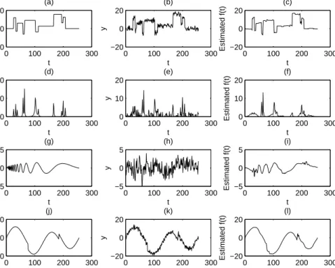
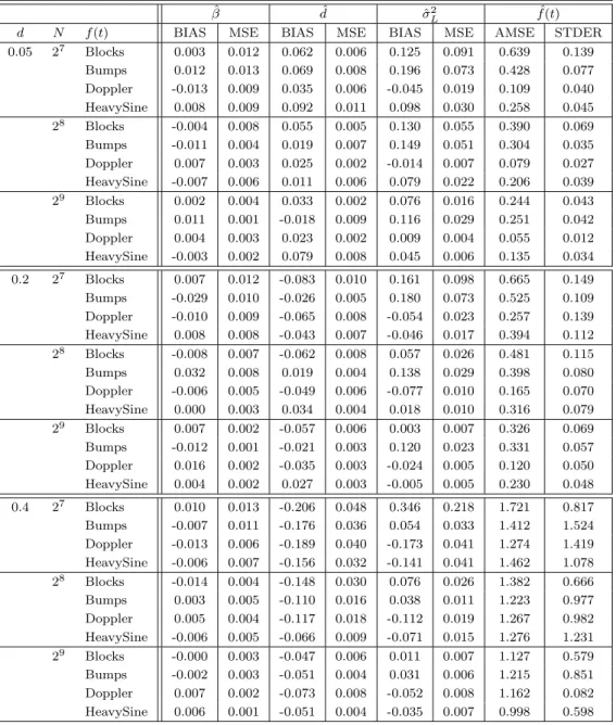
Table 1 shows the result. For all values ofdthe mean squared errors (MSE) and the biases of ˆβ, d,ˆ σˆL2 consistently decreased in almost all cases as the sample size increased. In the estimation of the nonparametric component, AMSEs and their standard errors (STDER) decreased as d approached 0 (i.e., almost uncorrelated errors). The MCMC chains mixed well and converged to the true values of the model parameters. Figure 1 shows the ideal four nonparametric functions in the first column, the corresponding contaminated series with a trend (β = 1) and long memory error (d= 0.2, σ2
L = 1) in the second column, and
the nonparametric function estimates via the proposed method in the third column. Finally, we report simulation results of ARFIMA(0, d,1) in Table 2. In the simulation, the long memory parameter d and moving average parameter θ were set to 0.2 and 0.3, respectively. For the Metropolis move of θ, we used the normal proposal distribution with standard deviation 0.05. The other parameters remained the same as in the simulation with ARFIMA(0, d,0) errors. The biases and mean squared errors of ˆβ,d,ˆθˆand ˆσ2 and the AMSEs and standard errors of ˆf(t) were relatively large compared to those of the models without the moving average parameter, although they still showed good performances.
4.1 An Application to Northern Hemisphere Temperature Data
For an application we considered the Northern hemisphere temperature data, measured in months during the years 1854-1989, gathered by the Climate Research Unit of the University of East Anglia, England. This dataset is a benchmark in the long memory literature and has been used widely for the study of global warming. Beran (1994) fitted a linear trend model
yt=β0+β1t+εtto the data and applied the ARFIMA(0, d,0) model to the residuals that
resulted from detrending the data with the ordinary least square (OLS) estimate. The OLS estimate ofβ1 is 0.00032, and ˆdand ˆσL2 were 0.37 and 0.0089, respectively. Beran and Feng
(2002) obtained ˆd= 0.33 and a 95% confidence interval (CI) of (0.19, 0.46) by SEMIFAR model. On the other hand, one can find that the variability of the series at the beginning is larger than for the rest of the observations. Craigmile, Guttorp and Percival (2005) obtained ˆd = 0.361 with a 95% CI of (0.317, 0.408) and ˆσ2L = 0.045 with an estimation method that ignored the non-constant variance of the data, and an estimate of ˆd= 0.368 with a 95% CI of (0.323, 0.415) and ˆσL2 = 0.032 when taking into account the non-constant variability.
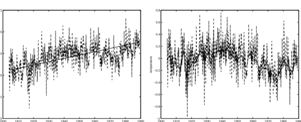
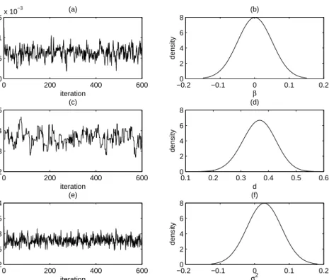
We applied our wavelet-based MCMC method for PLR models to the Northern hemi-sphere data. We chose ARFIMA(0, d,0) as the error term. We discarded the first 608 temperatures, obtaining N = 1024 measurements. This refinement of data was needed to meet the stationarity assumption of the long memory error in our model. Figure 2 shows the data versus the estimated trend line (left) and the data versus the estimated nonpara-metric function after detrending them with the estimated trend ˆβ (right). The estimates of β, d, and σ2L were 0.0006, 0.3660, and 0.0278, respectively. Our estimate of d is close to those found by Beran (1994) and Craigmile, Guttorp and Percival (2005). Our estimate of σL2 is closer to the one obtained by Craigmile, Guttorp and Percival (2005) when the nonconstant variability is taken into account. Overall, the temperature in the Northern hemisphere seems to increase approximately 0.72 degree in Celsius per century. Figure 3 shows the MCMC traces and the density plots of the estimated parameters.
5
Concluding Remarks
We have proposed a wavelet-based Bayesian method for the estimation of the model param-eters and the nonparametric function in PLR models with long memory errors. We have taken advantage of the sparsity property of discrete wavelet transforms that reduces the strongly correlated response variable of the model to a nearly uncorrelated one. We have designed a Markov chain Monte Carlo method to obtain the posterior distributions of the model parameters and the nonparametric function. We have shown via simulation studies that the proposed method is promising and have demonstrated how it can be applied, by using the benchmark Northern hemisphere temperature data. The contribution of our work, with respect to existing literature, relies in incorporating strongly correlated long memory errors into PLR models, and in exploiting the whitening properties of the discrete wavelet transforms to design a computationally inexpensive inferential procedure.
Although we have chosen ARFIMA processes for the long memory error of the model, the proposed procedure can be easily applied to other long memory processes, such as fractional Brownian motion (fBm) or fractional Gaussian noise (fGn). Extensions to non-equally spaced designs for the nonparametric predictor function can be also considered. In this setting inference cannot rely on models that imply thea posterioriindependence of the coefficients, unlike in the case of equispaced data. Mixture prior models can still be applied to the coefficients of the wavelet expansion but appropriate inferential procedures need to be developed, perhaps along the lines of what done by Park, Vannucci and Hart (2005).
Acknowledgment
The authors thank an associate editor and two referees for their valuable comments on an earlier version of the paper. Vannucci is supported by NSF, DMS-0605001, and by NIH, R01 HG003319-01.
Appendix. MCMC on Full Conditional Distributions
Let U∗ = Σ−1/2 Ψ U, ϑ∗ = Σ −1/2 Ψ ϑ, and ω∗ = Σ −1/2 Ψ ω, where Σ−1Ψ = Σ −1/2 Ψ Σ −1/2 Ψ . We
sample the parameters by iterating among the following steps:
(1) sample β from β|Ψ, σ2L, ϑ, γ, ω, U ∼N(U∗′U∗)−1U∗′(ω∗−ϑ∗), σL2(U∗′U∗)−1; (2) sample Ψ from Ψ|β, σL2, ϑ, γ, ω, U ∝ |ΣΨ|−1/2(2d)η−1(1−2d)ν−1 exp " − 1 2σ2 L (ω∗−U∗β−ϑ∗)′(ω∗−U∗β−ϑ∗) # ; (3) sample σ2 L from σL2|β,Ψ, ϑ, γ, ω, U ∼IG N 2, (ω∗−U∗β−ϑ∗)′(ω∗−U∗β−ϑ∗) 2 ,where IG(a, b) denotes the inverse gamma distribution with parameters aand band pdf p(x|a, b)∼
(ba/Γ(a))x−(a+1)e−b/x;
(4) sample γjk from P(γjk= 1|β,Ψ, σ2L, ωjk, uijk) =Ojk/(Ojk+ 1) where
Ojk = v u u t σ2 Lσ2jk τ2 j +σL2σ2jk ×exp " τj2(ωjk−Pli=1βiuijk)2 2σ2 Lσjk2 (τj2+σL2σjk2 ) # × pj 1−pj ; (5) sample ϑfrom ϑjk|β,Ψ, σ2L, γjk, ωjk, ujk∼N γjkτj2(ωjk−Pli=1βiuijk) σ2 Lσ2jk+τj2 , σ 2 Lσ2jk·τj2 σ2 Lσ2jk+τj2 γjk ! .
Note that, like the prior model, the full conditional distribution of ϑjk is a mixture of a
does not have a known closed form, we use a Metropolis sampler with independent Gaussian proposal distributions.
References
Abramovich, F., Sapatinas, T. and Silverman, B.W. (1998). Wavelet thresholding via a Bayesian approach. J. Roy. Statist. Soc. Ser. B60, 725-49.
Antoniadis, A. and Bigot, J. and Sapatinas, T. (2001). Wavelet estimators in nonpara-metric regression: A comparative simulation study. J. Statist. Soft. 6, 1-83.
Beran, J. (1994). Statistics for Long-Memory Processes. Chapman and Hall, New York. Beran, J. and Feng, Y. (2002). SEMIFAR models-A semiparametric approach to modelling
trends, long-range dependence. Comput. Statist. Data Anal. 40, 393-419.
Beran, J. and Ghosh, S. (1998). Root-n-consistent estimation in partial linear models with long-memory errors. Scand. J. Statist. 25, 345-357.
Chang, X.W. and Qu, L. (2004). Wavelet estimation of partially linear models. Comp. Stat. Data Anal. 47, 31-48.
Clyde, M., Parmigiani, G. and Vidakovic, B. (1998). Multiple shrinkage and subset selec-tion in wavelets. Biometrika 85, 391-402.
Craigmile, P.F. and Percival, D.B. (2005). Asymptotic decorrelation of between-scale Wavelet Coefficients, IEEE Trans. Info. Theory51, 1039-1048.
Craigmile, P.F., Guttorp, P. and Percival, D.B. (2005). Wavelet-based parameter esti-mation for polynomial contaminated fractionally differenced processes. IEEE. Trans. Sig. Proc. 53, 3151-3161.
Donoho, D.L. and Johnstone, I.M. (1994). Ideal spatial adaptation by wavelet shrinkage.
Biometrika 81, 425-455.
Donoho, D.L. and Johnstone, I.M. (1995). Adapting to unknown smoothness via wavelet shrinkage. J. Roy. Statist. Soc. Ser. B 57, 301-369.
Doornik, J.A. and Ooms, M. (2003). Computational aspects of maximum likelihood esti-mation of autoregressive fractionally integrated moving average models. Comp. Stat. Data Anal. 42, 333-348.
Engle, R.F., Granger, C.W.J., Rice, J. and Weiss, A. (1986). Semiparametric estimates of the relation between weather and electricity sales. J. Amer. Statist. Assoc. 81, 310-320.
Fadili, M.J. and Bullmore, E.T. (2005). Penalized partially linear models using sparse representations with an application to fMRI time series. IEEE. Trans. Sig. Proc. 53, 3436-3448.
Germ´an, A.P., Wenceslao, G.M. and Philippe, V. (2004). Estimation and testing in a partial linear regression model under long-memory dependence. Bernoulli 10, 49-78. Granger, C.W. and Joyeux, R. (1980). An introduction to long memory time series models
and fractional differencing. J. Time Series Anal. 1, 15-29.
Hosking, J.R.M. (1981). Fractional differencing. Biometrika 68, 165-176.
Ko, K. and Vannucci, M. (2006). Bayesian wavelet analysis of autoregressive fractionally integrated moving-average processes. J. Statist. Plan. Inference 136, 3415-3434. Koop, G and Porier, D. (2004). Bayesian variants of some classical semiparametric
regres-sion techniques. J. Econ. 123, 259-282.
Lenk, P.J. (1999). Bayesian inference for semiparametric regression using a Fourier repre-sentation. J. Roy. Statist. Soc. Ser. B 61, 863-879.
Mallat, S.G. (1989). A theory for multiresolution signal decomposition: the Wavelet Rep-resentation. IEEE Trans. Patt. Anal. Mac. Int. 11, 674-693.
McLeod, A.I. and Hipel, K.W. (1978). Preservation of the rescaled adjusted range, Parts 1, 2 and 3. Water Resources Research14, 491-512.
Park, C.G., Vannucci, M. and Hart, J.D. (2005). Bayesian methods for wavelet series in single-index models. J. Comp. Graph. Statist. 14, 770-794.
Qu, L. (2003). Wavelet thresholding in partially linear models: a computation and simu-lation. Appl. Stoc. Models Bus. Ind. 19, 221-230.
Qu, L. (2006). Bayesian wavelet estimation of partially linear models. J. Statist. Comp. Sim. 76, 605-617.
Sowell, F. (1992). Maximum likelihood estimation of stationary univariate fractionally integrated time series models. J. Econ. 53, 165-188.
Taswell, C. and McGill, K.C. (1994). Wavelet transform algorithms for finite-duration discrete-time signals. ACM Trans. Math. Soft. 20, 398-412.
Tewfik, A.H. and Kim, M. (1992). Correlation structure of the discrete wavelet coefficients of fractional Brownian motion. IEEE Trans. Info. Theory 38, 904-909.
0 100 200 300 −20 0 20 t f(t) (a) 0 100 200 300 −20 0 20 t y (b) 0 100 200 300 −20 0 20 t Estimated f(t) (c) 0 100 200 300 0 10 20 t f(t) (d) 0 100 200 300 0 10 20 t y (e) 0 100 200 300 0 10 20 t Estimated f(t) (f) 0 100 200 300 −5 0 5 t f(t) (g) 0 100 200 300 −5 0 5 t y (h) 0 100 200 300 −5 0 5 t Estimated f(t) (i) 0 100 200 300 −20 0 20 t f(t) (j) 0 100 200 300 −20 0 20 t y (k) 0 100 200 300 −20 0 20 t Estimated f(t) (l)
Figure 1: The four nonparametric functions: (a) Blocks, (d) Bumps, (g) Doppler, and (j) HeavySine.
Plots in the second column show noisy data with Gaussian long memory errors with d = .2 and
σ2
L = 1. Hereβ = 1. Plots in the third column show the recovered functions using the proposed
wavelet-based Bayesian method.
Vannucci, M. and Corradi, F. (1999). Covariance structure of wavelet coefficients: Theory and models in a Bayesian perspective. J. Roy. Statist. Soc. Ser. B61, 971-986.
ˆ
β dˆ σˆ2
L fˆ(t)
d N f(t) BIAS MSE BIAS MSE BIAS MSE AMSE STDER 0.05 27 Blocks 0.003 0.012 0.062 0.006 0.125 0.091 0.639 0.139 Bumps 0.012 0.013 0.069 0.008 0.196 0.073 0.428 0.077 Doppler -0.013 0.009 0.035 0.006 -0.045 0.019 0.109 0.040 HeavySine 0.008 0.009 0.092 0.011 0.098 0.030 0.258 0.045 28 Blocks -0.004 0.008 0.055 0.005 0.130 0.055 0.390 0.069 Bumps -0.011 0.004 0.019 0.007 0.149 0.051 0.304 0.035 Doppler 0.007 0.003 0.025 0.002 -0.014 0.007 0.079 0.027 HeavySine -0.007 0.006 0.011 0.006 0.079 0.022 0.206 0.039 29 Blocks 0.002 0.004 0.033 0.002 0.076 0.016 0.244 0.043 Bumps 0.011 0.001 -0.018 0.009 0.116 0.029 0.251 0.042 Doppler 0.004 0.003 0.023 0.002 0.009 0.004 0.055 0.012 HeavySine -0.003 0.002 0.079 0.008 0.045 0.006 0.135 0.034 0.2 27 Blocks 0.007 0.012 -0.083 0.010 0.161 0.098 0.665 0.149 Bumps -0.029 0.010 -0.026 0.005 0.180 0.073 0.525 0.109 Doppler -0.010 0.009 -0.065 0.008 -0.054 0.023 0.257 0.139 HeavySine 0.008 0.008 -0.043 0.007 -0.046 0.017 0.394 0.112 28 Blocks -0.008 0.007 -0.062 0.008 0.057 0.026 0.481 0.115 Bumps 0.032 0.008 0.019 0.004 0.138 0.029 0.398 0.080 Doppler -0.006 0.005 -0.049 0.006 -0.077 0.010 0.165 0.070 HeavySine 0.000 0.003 0.034 0.004 0.018 0.010 0.316 0.079 29 Blocks 0.007 0.002 -0.057 0.006 0.003 0.007 0.326 0.069 Bumps -0.012 0.001 -0.021 0.003 0.120 0.023 0.331 0.057 Doppler 0.016 0.002 -0.035 0.003 -0.024 0.005 0.120 0.050 HeavySine 0.004 0.002 0.027 0.003 -0.005 0.005 0.230 0.048 0.4 27 Blocks 0.010 0.013 -0.206 0.048 0.346 0.218 1.721 0.817 Bumps -0.007 0.011 -0.176 0.036 0.054 0.033 1.412 1.524 Doppler -0.013 0.006 -0.189 0.040 -0.173 0.041 1.274 1.419 HeavySine -0.006 0.007 -0.156 0.032 -0.141 0.041 1.462 1.078 28 Blocks -0.014 0.004 -0.148 0.030 0.076 0.026 1.382 0.666 Bumps 0.003 0.005 -0.110 0.016 0.038 0.011 1.223 0.977 Doppler 0.005 0.004 -0.117 0.018 -0.112 0.019 1.267 0.982 HeavySine -0.006 0.005 -0.066 0.009 -0.071 0.015 1.276 1.231 29 Blocks -0.000 0.003 -0.047 0.006 0.011 0.007 1.127 0.579 Bumps -0.002 0.003 -0.051 0.004 0.031 0.006 1.215 0.851 Doppler 0.007 0.002 -0.073 0.008 -0.052 0.008 1.162 0.082 HeavySine 0.006 0.001 -0.051 0.004 -0.035 0.007 0.998 0.598
Table 1: Biases, MSEs and AMSEs of the estimated model parameters from the wavelet-based
Bayesian estimation procedure when the error is simulated from an ARFIMA(0, d,0). Bothβ and
σ2
ˆ
β dˆ θˆ σˆ2
L fˆ(t)
N f(t) BIAS MSE BIAS MSE BIAS MSE BIAS MSE AMSE STDER 27 Blocks -0.004 0.016 -0.091 0.021 -0.209 0.258 0.180 0.148 1.164 0.333 Bumps -0.013 0.018 -0.092 0.031 0.311 0.120 0.825 0.776 1.921 0.316 Doppler 0.010 0.006 -0.074 0.008 0.123 0.061 -0.153 0.049 0.558 0.164 HeavySine -0.022 0.009 -0.025 0.008 0.213 0.079 -0.046 0.048 0.960 0.297 28 Blocks -0.006 0.004 -0.018 0.010 0.179 0.056 -0.094 0.033 0.903 0.287 Bumps 0.002 0.006 0.105 0.010 0.259 0.110 0.316 0.137 1.291 0.274 Doppler -0.014 0.003 -0.086 0.012 0.097 0.041 -0.121 0.028 0.462 0.153 HeavySine -0.013 0.004 -0.016 0.004 0.178 0.064 -0.022 0.022 0.682 0.181 29 Blocks 0.003 0.003 0.016 0.002 0.092 0.051 -0.076 0.021 0.867 0.229 Bumps -0.003 0.002 -0.044 0.004 0.128 0.051 0.281 0.109 1.122 0.151 Doppler 0.006 0.001 -0.091 0.011 0.097 0.019 -0.088 0.012 0.343 0.108 HeavySine 0.007 0.002 -0.019 0.008 0.078 0.032 0.007 0.010 0.436 0.108
Table 2: Biases, MSEs and AMSEs of the estimated model parameters from the wavelet-based
Bayesian estimation procedure when the error is simulated from an ARFIMA(0, d,1). The moving
average parameterθ is set to 0.3, and bothβ andσ2
L are set to 1. 1900 1910 1920 1930 1940 1950 1960 1970 1980 1990 −1.5 −1 −0.5 0 0.5 1 year temperature 1900 1910 1920 1930 1940 1950 1960 1970 1980 1990 −1 −0.8 −0.6 −0.4 −0.2 0 0.2 0.4 0.6 0.8 year temperature
Figure 2: Left: Northern Hemisphere temperature data with N = 1024 (dashed line) and fitted
trend (solid line), Right: Northern Hemisphere temperature data after detrending by the estimated
0 200 400 600 0 0.5 1 1.5x 10 −3 iteration β (a) −0.20 −0.1 0 0.1 0.2 2 4 6 8 β density (b) 0 200 400 600 0.2 0.3 0.4 0.5 iteration d (c) 0.1 0.2 0.3 0.4 0.5 0.6 0 2 4 6 8 d density (d) 0 200 400 600 0.02 0.025 0.03 0.035 0.04 iteration σL 2 (e) −0.20 −0.1 0 0.1 0.2 2 4 6 8 σ L 2 density (f)
Figure 3: Northern Hemisphere Temperature: MCMC traces of ˆβ, d,ˆ σˆ2
Land corresponding density