Unsupervised Learning

(1)

Unsupervised Learning

∗

Zoubin Ghahramani

†

Gatsby Computational Neuroscience Unit University College London, UK

[email protected] http://www.gatsby.ucl.ac.uk/~zoubin

September 16, 2004

Abstract

We give a tutorial and overview of the field of unsupervised learning from the perspective of statistical modelling. Unsupervised learning can be motivated from information theoretic and Bayesian principles. We briefly review basic models in unsupervised learning, including factor analysis, PCA, mixtures of Gaussians, ICA, hidden Markov models, state-space models, and many variants and extensions. We derive the EM algorithm and give an overview of fundamental concepts in graphical models, and inference algorithms on graphs. This is followed by a quick tour of approximate Bayesian inference, including Markov chain Monte Carlo (MCMC), Laplace approximation, BIC, variational approximations, and expectation propagation (EP). The aim of this chapter is to provide a high-level view of the field. Along the way, many state-of-the-art ideas and future directions are also reviewed.

1 Introduction

Machine learning is the field of research devoted to the formal study of learning systems. This is a highly interdisciplinary field which borrows and builds upon ideas from statistics, computer science, engineering, cognitive science, optimisation theory and many other disciplines of science and mathematics. The purpose of this chapter is to introduce in a fairly concise manner the key ideas underlying the sub-field of machine learning known as unsupervised learning. This introduction is necessarily incomplete given the enormous range of topics under the rubric of unsupervised learning. The hope is that interested readers can delve more deeply into the many topics covered here by following some of the cited references. The chapter starts at a highly tutorial level but will touch upon state-of-the-art research in later sections. It is assumed that the reader is familiar with elementary linear algebra, probability theory, and calculus, but not much else.

1.1 What is unsupervised learning?

Consider a machine (or living organism) which receives some sequence of inputs x1, x2, x3, . . ., where xt is

the sensory input at timet. This input, which we will often call thedata, could correspond to an image on the retina, the pixels in a camera, or a sound waveform. It could also correspond to less obviously sensory data, for example the words in a news story, or the list of items in a supermarket shopping basket.

One can distinguish between four different kinds of machine learning. Insupervised learningthe machine1

is also given a sequence of desired outputsy1, y2, . . . ,and the goal of the machine is to learn to produce the

correct output given a new input. This output could be a class label (in classification) or a real number (in regression).

In reinforcement learning the machine interacts with its environment by producing actions a1, a2, . . ..

These actions affect the state of the environment, which in turn results in the machine receiving some scalar rewards (or punishments) r1, r2, . . .. The goal of the machine is to learn to act in a way that maximises

the future rewards it receives (or minimises the punishments) over its lifetime. Reinforcement learning is closely related to the fields of decision theory (in statistics and management science), and control theory (in engineering). The fundamental problems studied in these fields are often formally equivalent, and the solutions are the same, although different aspects of problem and solution are usually emphasised.

A third kind of machine learning is closely related togame theoryand generalises reinforcement learning. Here again the machine gets inputs, produces actions, and receives rewards. However, the environment the machine interacts with is not some static world, but rather it can contain other machines which can also sense, act, receive rewards, and learn. Thus the goal of the machine is to act so as to maximise rewards in light of the other machines’ current and future actions. Although there is a great deal of work in game theory for simple systems, the dynamic case with multiple adapting machines remains an active and challenging area of research.

Finally, inunsupervised learningthe machine simply receives inputsx1, x2, . . ., but obtains neither

super-vised target outputs, nor rewards from its environment. It may seem somewhat mysterious to imagine what the machine could possibly learn given that it doesn’t get any feedback from its environment. However, it is possible to develop of formal framework for unsupervised learning based on the notion that the machine’s goal is to build representations of the input that can be used for decision making, predicting future inputs, efficiently communicating the inputs to another machine, etc. In a sense, unsupervised learning can be thought of as finding patterns in the data above and beyond what would be considered pure unstructured noise. Two very simple classic examples of unsupervised learning are clustering and dimensionality reduction. We discuss these in Section 2. The remainder of this chapter focuses on unsupervised learning, although many of the concepts discussed can be applied to supervised learning as well. But first, let us consider how unsupervised learning relates to statistics and information theory.

1_{Henceforth, for succinctness I’ll use the term machine to refer both to machines and living organisms. Some people prefer to} call this a system or agent. The same mathematical theory of learning applies regardless of what we choose to call the learner, whether it is artificial or biological.

(4)

1.2 Machine learning, statistics, and information theory

Almost all work in unsupervised learning can be viewed in terms of learning a probabilistic model of the data. Even when the machine is given no supervision or reward, it may make sense for the machine to estimate a model that represents the probability distribution for a new input xt given previous inputs

x1, . . . , xt−1 (consider the obviously useful examples of stock prices, or the weather). That is, the learner

models P(xt|x1, . . . , xt−1). In simpler cases where the order in which the inputs arrive is irrelevant or

unknown, the machine can build a model of the data which assumes that the data points x1, x2, . . . are

independently and identically drawn from some distributionP(x)2.

Such a model can be used foroutlier detectionormonitoring. Letxrepresent patterns of sensor readings from a nuclear power plant and assume thatP(x) is learned from data collected from a normally functioning plant. This model can be used to evaluate the probability of a new sensor reading; if this probability is abnormally low, then either the model is poor or the plant is behaving abnormally, in which case one may want to shut it down.

A probabilistic model can also be used for classification. Assume P1(x) is a model of the attributes of

credit card holders who paid on time, andP2(x) is a model learned from credit card holders who defaulted

on their payments. By evaluating the relative probabilities P1(x0) and P2(x0) on a new applicant x0, the

machine can decide to classify her into one of these two categories.

With a probabilistic model one can also achieve efficientcommunicationanddata compression. Imagine that we want to transmit, over a digital communication line, symbols xrandomly drawn from P(x). For example, x may be letters of the alphabet, or images, and the communication line may be the internet. Intuitively, we should encode our data so that symbols which occur more frequently have code words with fewer bits in them, otherwise we are wasting bandwidth. Shannon’s source coding theorem quantifies this by telling us that the optimal number of bits to use to encode a symbol with probability P(x) is−log₂P(x). Using these number of bits for each symbol, the expected coding cost is the entropy of the distributionP.

H(P)def= −X

x

P(x) log₂P(x) (1)

In general, the true distribution of the data is unknown, but we can learn a model of this distribution. Let’s call this modelQ(x). The optimal codewith respect to this modelwould use−log₂Q(x) bits for each symbol x. The expected coding cost, taking expectations with respect to the true distribution, is

−X

x

P(x) log₂Q(x) (2)

The difference between these two coding costs is called the Kullback-Leibler (KL) divergence KL(PkQ)def= X

x

P(x) logP(x)

Q(x) (3)

The KL divergence is non-negative and zero if and only if P=Q. It measures the coding inefficiency in bits from using a model Q to compress data when the true data distribution is P. Therefore, the better our model of the data, the more efficiently we can compress and communicate new data. This is an important link between machine learning, statistics, and information theory. An excellent text which elaborates on these relationships and many of the topics in this chapter is [48].

1.3 Bayes rule

Bayes rule,

P(y|x) =P(x|y)P(y)

P(x) (4)

which follows from the equality P(x, y) =P(x)P(y|x) = P(y)P(x|y), can be used to motivate a coherent statistical framework for machine learning. The basic idea is the following. Imagine we wish to design a 2_{We will use both} _P _and _p _{to denote probability distributions and probability densities. The meaning should be clear} depending on whether the argument is discrete or continuous.

(5)

machine which has beliefs about the world, and updates these beliefs on the basis of observed data. The machine must somehow represent the strengths of its beliefs numerically. It has been shown that if you accept certain axioms of coherent inference, known as the Cox axioms, then a remarkable result follows [36]: If the machine is to represent the strength of its beliefs by real numbers, then the only reasonable and coherent way of manipulating these beliefs is to have them satisfy the rules of probability, such as Bayes rule. Therefore,P(X =x) can be used not only to represent the frequency with which the variableX takes on the valuex(as in so-called frequentist statistics) but it can also be used to represent the degree of belief thatX =x. Similarly,P(X=x|Y =y) can be used to represent the degree of belief thatX =xgiven that one knownsY =y.3

From Bayes rule we derive the following simple framework for machine learning. Assume a universe of models Ω; let Ω ={1, . . . , M}although it need not be finite or even countable. The machines starts with some prior beliefs over modelsm ∈Ω (we will see many examples of models later), such thatPM

m=1P(m) = 1.

A model is simply some probability distribution over data points, i.e.P(x|m). For simplicity, let us further assume that in all the models the data is taken to be independently and identically distributed (iid). After observing a data setD={x1, . . . , xN}, the beliefs over models is given by:

P(m|D) =P(m)P(D|m) P(D) ∝P(m) N Y n=1 P(xn|m) (5)

which we read as theposterior over modelsis thepriormultiplied by the likelihood, normalised. Thepredictive distributionover new data, which would be used to encode new data efficiently, is

P(x|D) =

M

X

m=1

P(x|m)P(m|D) (6)

Again this follows from the rules of probability theory, and the fact that the models are assumed to produce iid data.

Often models are defined by writing down a parametric probability distribution (again, we’ll see many examples below). Thus, the model m might have parameters θ, which are assumed to be unknown (this could in general be a vector of parameters). To be a well-defined model from the perspective of Bayesian learning, one has to define a prior over these model parameters P(θ|m) which naturally has to satisfy the following equality

P(x|m) = Z

P(x|θ, m)P(θ|m)dθ (7)

Given the modelmit is also possible to infer the posterior over the parameters of the model, i.e.P(θ|D, m), and to compute the predictive distribution, P(x|D, m). These quantities are derived in exact analogy to equations (5) and (6), except that instead of summing over possible models, we integrate over parameters of a particular model. All the key quantities in Bayesian machine learning follow directly from the basic rules of probability theory.

Certain approximate forms of Bayesian learning are worth mentioning. Let’s focus on a particular model m with parameters θ, and an observed data set D. The predictive distribution averages over all possible parameters weighted by the posterior

P(x|D, m) = Z

P(x|θ)P(θ|D, m)dθ. (8)

In certain cases, it may be cumbersome to represent the entire posterior distribution over parameters, so instead we will choose to find a point-estimate of the parameters ˆθ. A natural choice is to pick the most 3_{Another way to motivate the use of the rules of probability to encode degrees of belief comes from game-theoretic arguments} in the form of theDutch Book Theorem. This theorem states that if you are willing to accept bets with odds based on your degrees of beliefs, then unless your beliefs are coherent in the sense that they satisfy the rules of probability theory, there exists a set of simultaneous bets (called a “Dutch Book”) which you will accept and which is guaranteed to lose you money, no matter what the outcome. The only way to ensure that Dutch Books don’t exist against you, is to have degrees of belief that satisfy Bayes rule and the other rules of probability theory.

(6)

probable parameter value given the data, which is known as themaximum a posteriorior MAP parameter estimate

ˆ

θMAP= arg max

θ P(θ|D, m) = arg maxθ " logP(θ|m) +X n logP(xn|θ, m) # (9) Another natural choice is themaximum likelihoodor ML parameter estimate

ˆ θML= arg max θ P(D|θ, m) = arg maxθ X n logP(xn|θ, m) (10)

Many learning algorithms can be seen as finding ML parameter estimates. The ML parameter estimate is also acceptable from a frequentist statistical modelling perspective since it does not require deciding on a prior over parameters. However, ML estimation does not protect against overfitting—more complex models will generally have higher maxima of the likelihood. In order to avoid problems with overfitting, frequentist procedures often maximise apenalised orregularised log likelihood (e.g. [26]). If the penalty or regularisation term is interpreted as a log prior, then maximising penalised likelihood appears identical to maximising a posterior. However, there are subtle issues that make a Bayesian MAP procedure and maximum penalised likelihood different [28]. One difference is that the MAP estimate is not invariant to reparameterisation, while the maximum of the penalised likelihood is invariant. The penalised likelihood is a function, not a density, and therefore does not increase or decrease depending on the Jacobian of the reparameterisation.

2 Latent variable models

The framework described above can be applied to a wide range of models. No singe model is appropriate for all data sets. The art in machine learning is to develop models which are appropriate for the data set being analysed, and which have certain desired properties. For example, for high dimensional data sets it might be necessary to use models that perform dimensionality reduction. Of course, ultimately, the machine should be able to decide on the appropriate model without any human intervention, but to achieve this in full generality requires significant advances in artificial intelligence.

In this section, we will consider probabilistic models that are defined in terms of some latent or hidden variables. These models can be used to do dimensionality reduction and clustering, the two cornerstones of unsupervised learning.

2.1 Factor analysis

Let the data set Dconsist ofD-dimensional real valued vectors, D={y1, . . . ,yN}. In factor analysis, the

data is assumed to be generated from the following model

y= Λx+ (11)

wherexis aK-dimensional zero-mean unit-variance multivariate Gaussian vector with elements correspond-ing to hidden (or latent) factors, Λ is aD×K matrix of parameters, known as the factor loading matrix, andis aD-dimensional zero-mean multivariate Gaussian noise vector with diagonal covariance matrix Ψ. Defining the parameters of the model to beθ= (Ψ,Λ), by integrating out the factors, one can readily derive that

p(y|θ) = Z

p(x|θ)p(y|x, θ)dx=N(0,ΛΛ>+ Ψ) (12) where N(µ,Σ) refers to a multivariate Gaussian density with meanµ and covariance matrix Σ. For more details refer to [68].

Factor analysis is an interesting model for several reasons. If the data is very high dimensional (D is large) then even a simple model like the full-covariance multivariate Gaussian will have too many parameters to reliably estimate or infer from the data. By choosingK < D, factor analysis makes it possible to model a Gaussian density for high dimensional data without requiringO(D2_{) parameters. Moreover, given a new}

data point, one can compute the posterior over the hidden factors, p(x|y, θ); since x is lower dimensional thanythis provides a low-dimensional representation of the data (for example, one could pick the mean of p(x|y, θ) as the representation fory).

(7)

2.2 Principal components analysis (PCA)

Principal components analysis (PCA) is an important limiting case of factor analysis (FA). One can derive PCA by making two modifications to FA. First, the noise is assumed to be isotropic, in other words each element ofhas equal variance: Ψ =σ2_I_{, where}_I_{is a}_D_×_D_{identity matrix. This model is called}_{probabilistic}

PCA[67, 78]. Second, if we take the limit ofσ→0 in probabilistic PCA, we obtain standard PCA (which also goes by the names Karhunen-Lo`eve expansion, and singular value decomposition; SVD). Given a data set with covariance matrix Σ, for maximum likelihood factor analysis the goal is to find parameters Λ, and Ψ for which the model ΛΛ>+ Ψ has highest likelihood. In PCA, the goal is to find Λ so that the likelihood is highest for ΛΛ>. Note that this matrix is singular unlessK=D, so the standard PCA model is not a sensible model. However, taking the limiting case, and further constraining the columns of Λ to be orthogonal, it can be derived that the principal components correspond to theK eigenvectors with largest eigenvalue of Σ. PCA is thus attractive because the solution can be found immediately after eigendecomposition of the covariance. Taking the limit σ→0 ofp(x|y,Λ, σ) we find that it is a delta-function atx= Λ>_y_{, which is}

the projection ofyonto the principal components.

2.3 Independent components analysis (ICA)

Independent components analysis (ICA) extends factor analysis to the case where the factors are non-Gaussian. This is an interesting extension because many real-world data sets have structure which can be modelled as linear combinations of sparse sources. This includes auditory data, images, biological signals such as EEG, etc. Sparsity simply corresponds to the assumption that the factors have distributions with higher kurtosis that the Gaussian. For example,p(x) =λ

2exp{−λ|x|}has a higher peak at zero and heavier

tails than a Gaussian with corresponding mean and variance, so it would be considered sparse (strictly speaking, one would like a distribution which had non-zero probability mass at 0 to get true sparsity).

Models like PCA, FA and ICA can all be implemented using neural networks (multilayer perceptrons) trained using various cost functions. It is not clear what advantage this implementation/interpretation has from a machine learning perspective, although it provides interesting ties to biological information processing. Rather than ML estimation, one can also do Bayesian inference for the parameters of probabilistic PCA, FA, and ICA.

2.4 Mixture of Gaussians

The densities modelled by PCA, FA and ICA are all relatively simple in that they are unimodal and have fairly restricted parametric forms (Gaussian, in the case of PCA and FA). To model data with more complex structure such as clusters, it is very useful to consider mixture models. Although it is straightforward to consider mixtures of arbitrary densities, we will focus on Gaussians as a common special case. The density of each data point in a mixture model can be written:

p(y|θ) =

K

X

k=1

πk p(y|θk) (13)

where each of the K components of the mixture is, for example, a Gaussian with differing means and covariances θk = (µk,Σk) and πk is the mixing proportion for component k, such thatPK_k₌₁πk = 1 and

πk>0, ∀k.

A different way to think about mixture models is to consider them as latent variable models, where associated with each data point is aK-ary discrete latent (i.e. hidden) variableswhich has the interpretation thats=k if the data point was generated by componentk. This can be written

p(y|θ) =

K

X

k=1

P(s=k|π)p(y|s=k, θ) (14)

whereP(s=k|π) =πk is the prior for the latent variable taking on value k, and p(y|s=k, θ) =p(y|θk) is

(8)

2.5 K-means

The mixture of Gaussians model is closely related to an unsupervised clustering algorithm known ask-means as follows: Consider the special case where all the Gaussians have common covariance matrix proportional to the identity matrix: Σk = σ2I, ∀k, and let πk = 1/K, ∀k. We can estimate the maximum likelihood

parameters of this model using the iterative algorithm which we are about to describe, known as EM. The resulting algorithm, as we take the limitσ2_→_{0, becomes exactly the}_k_{-means algorithm. Clearly the model}

underlyingk-means has only singular Gaussians and is therefore an unreasonable model of the data; however, k-means is usually justified from the point of view of clustering to minimise a distortion measure, rather than fitting a probabilistic models.

3 The EM algorithm

The EM algorithm is an algorithm for estimating ML parameters of a model with latent variables. Consider a model with observed variablesy, hidden/latent variablesx, and parameters θ. We can lower bound the log likelihood for any data point as follows

L(θ) = logp(y|θ) = log Z p(x,y|θ)dx (15) = log Z q(x)p(x,y|θ) q(x) dx (16) ≥ Z q(x) logp(x,y|θ) q(x) dx def = F(q, θ) (17)

whereq(x) is some arbitrary density over the hidden variables, and the lower bound holds due to the concavity of the log function (this inequality is known as Jensen’s inequality). The lower bound F is a functional of both the densityq(x) and the model parametersθ. For a data set ofN data pointsy(1), . . . ,y(N), this lower bound is formed for the log likelihood term corresponding to each data point, thus there is a separate density q(n)(x) for each point andF(q, θ) =P

nF

(n)₍_q(n)_{, θ}_).

The basic idea of the Expectation-Maximisation (EM) algorithm is to iterate between optimising this lower bound as a function of q and as a function of θ. We can prove that this will never decrease the log likelihood. After initialising the parameters somehow, thekth _{iteration of the algorithm consists of the}

following two steps:

E step: optimiseF with respect to the distributionq while holding the parameters fixed qk(x) = arg max q(x) Z q(x) logp(x,y|θk−1) q(x) (18) qk(x) = p(x|y, θk−1) (19)

M step: optimiseF with respect to the parameters θwhile holding the distribution over hidden variables fixed θk = arg max θ Z qk(x) log p(x,y|θ) qk(x) dx (20) θk = arg max θ Z qk(x) logp(x,y|θ)dx (21)

Let us be absolutely clear what happens for a data set ofN data points: In the E step, for each data point, the distribution over the hidden variables is set to the posterior for that data pointq(_kn)(x) =p(x|y(n)_{, θ}

k−1),

∀n. In the M step the single set of parameters is re-estimated by maximising the sum of the expected log likelihoods: θk= arg maxθPn

R

q_k(n)(x) logp(x,y(n)_|_θ₎_d_x_.

Two things are still unclear: how does (19) follow from (18), and how is this algorithm guaranteed to in-crease the likelihood? The optimisation in (18) can be written as follows sincep(x,y|θk−1) =p(y|θk−1)p(x|y, θk−1):

qk(x) = arg max q(x) h logp(y|θk−1) + Z q(x) logp(x|y, θk−1) q(x) dx i (22)

(9)

Now, the first term is a constant w.r.t. q(x) and the second term is the negative of the Kullback-Leibler divergence KL(q(x)kp(x|y, θk−1)) = Z q(x) log q(x) p(x|y, θk−1) dx (23)

which we have seen in Equation (3) in its discrete form. This is minimised atq(x) =p(x|y, θk−1), where the

KL divergence is zero. Intuitively, the interpretation of this is that in the E step of EM, the goal is to find the posterior distribution of the hidden variables given the observed variables and the current settings of the parameters. We also see that since the KL divergence is zero, at the end of the E step,F(qk, θk−1) =L(θk−1).

In the M step, F is increased with respect to θ. Therefore, F(qk, θk) ≥ F(qk, θk−1). Moreover,

L(θk) = F(qk+1, θk) ≥ F(qk, θk) after the next E step. We can put these steps together to establish

that L(θk) ≥ L(θk−1), establishing that the algorithm is guaranteed to increase the likelihood or keep it

fixed (at convergence).

The EM algorithm can be applied to all the latent variable models described above, i.e. FA, probabilistic PCA, mixture models, and ICA. In the case of mixture models, the hidden variable is the discrete assign-ment s of data points to clusters; consequently the integrals turn into sums where appropriate. EM has wide applicability to latent variable models, although it is not always the fastest optimisation method [70]. Moreover, we should note that the likelihood often has many local optima and EM will converge some local optimum which may not be the global one.

EM can also be used to estimate MAP parameters of a model, and as we will see in Section 11.4 there is a Bayesian generalization of EM as well.

4 Modelling time series and other structured data

So far we have assumed that the data isunstructured, that is, the observations are assumed to be independent and identically distributed. This assumption is unreasonable for many data sets in which the observations arrive in a sequence and subsequent observations are correlated. Sequential data can occur in time series modelling (as in financial data or the weather) and also in situations where the sequential nature of the data is not necessarily tied to time (as in protein data which consist of sequences of amino acids).

As the most basic level, time series modelling consists of building a probabilistic model of the present observation given all past observationsp(yt|yt−1,yt−2. . .). Because the history of observations grows

arbi-trarily large it is necessary to limit the complexity of such a model. There are essentially two ways of doing this.

The first approach is to limit the window of past observations. Thus one can simply model p(yt|yt−1)

and assume that this relation holds for allt. This is known as a first-order Markov model. A second-order Markov model would bep(yt|yt−1,yt−2), and so on. Such Markov models have two limitations: First, the

influence of past observations on present observations vanishes outside this window, which can be unrealistic. Second, it may be unnatural and unwieldy to model directly the relationship between raw observations at one time step and raw observations at a subsequent time step. For example, if the observations are noisy images, it would make more sense to de-noise them, extract some description of the objects, motions, illuminations, and then try to predict from that.

The second approach is to make use of latent or hidden variables. Instead of modelling directly the effect of yt−1 on yt, we assume that the observations were generated from some underlying hidden variable xt

which captures the dynamics of the system. For example, ymight be noisy sonar readings of objects in a room, whilexmight be the actual locations and sizes of these objects. We usually call this hidden variablex thestate variablesince it is meant to capture all the aspects of the system relevant to predicting the future dynamical behaviour of the system.

In order to understand more complex time series models, it is essential that one be familiar with state-space models (SSMs) and hidden Markov models (HMMs). These two classes of models have played a historically important role in control engineering, visual tracking, speech recognition, protein sequence mod-elling, and error decoding. They form the simplest building blocks from which other richer time-series models can be developed, in a manner completely analogous to the role that FA and mixture models play in building more complex models for iid data.

(10)

4.1 State-space models (SSMs)

In a state-space model, the sequence of observed datay1,y2,y3, . . .is assumed to have been generated from

some sequence of hidden state variables x1,x2,x3, . . .. Letting x1:T denote the sequence x1, . . . ,xT, the

basic assumption in an SSM is that the joint probability of the hidden states and observations factors in the following way: p(x1:T,y1:T|θ) = T Y t=1 p(xt|xt−1, θ)p(yt|xt, θ) (24)

In order words, the observations are assumed to have been generated from the hidden states viap(yt|xt, θ),

and the hidden states are assumed to have first-order Markov dynamics captured by p(xt|xt−1, θ). We can

consider the first termp(x1|x0, θ) to be a prior on the initial state of the systemx1.

The simplest kind of state-space model assumes that all variables are multivariate Gaussian distributed and all the relationships are linear. In suchlinear-Gaussian state-space models, we can write

yt = Cxt+vt (25)

xt = Axt−1+wt (26)

where the matricesCandAdefine the linear relationships andvandware zero-mean Gaussian noise vectors with covariance matricesRandQrespectively. If we assume that the prior on the initial statep(x1) is also

Gaussian, then all subsequentxs andys are also Gaussian due the the fact that Gaussian densities are closed under linear transformations. This model can be generalised in many ways, for example by augmenting it to include a sequence of observed inputs u1, . . . ,uT as well as the observed model outputsy1, . . . ,yT, but

we will not discuss generalisations further.

By comparing equations (11) and (25) we see that linear-Gaussian SSMs can be thought of as a time-series generalisation of factor analysis where the factors are assumed to have linear-Gaussian dynamics over time.

The parameters of this model are θ = (A, C, Q, R). To learn ML settings of these parameters one can make use of the EM algorithm [73]. The E step of the algorithm involves computingq(x1:T) =p(x1:T|y1:T, θ)

which is the posterior over hidden state sequences. In fact, this whole posterior does not have to be computed or represented, all that is required are the marginalsq(xt) and pairwise marginalsq(xt,xt+1). These can be

computed via theKalman smoothing algorithm, which is an efficient algorithm for inferring the distribution over the hidden states of a linear-Gaussian SSM. Since the model is linear, the M step of the algorithm requires solving a pair of weighted linear regression problems to re-estimate A andC, while Q and R are estimated from the residuals of those regressions. This is analogous to the M step of factor analysis, which also involves solving a linear regression problem.

4.2 Hidden Markov models (HMMs)

Hidden Markov models are similar to state-space models in that the sequence of observations is assumed to have been generated from a sequence of underlying hidden states. The key difference is that in HMMs the state is assumed to bediscreterather than a continuous random vector. Letstdenote the hidden state of an

HMM at timet. We assume thatstcan take discrete values in{1, . . . , K}. The model can again be written

as in (24): P(s1:T,y1:T|θ) = T Y t=1 P(st|st−1, θ)P(yt|st, θ) (27)

whereP(s1|s0, θ) is simply some initial distribution over theK settings of the first hidden state; we can call

this discrete distribitionπ, represented by a K×1 vector. The state-transition probabilities P(st|st−1, θ)

are captured by aK×K transition matrixA, with elementsAij =P(st=i|st−1=j, θ). The observations

in an HMM can be either continuous or discrete. For continuous observationsytone can for example choose

a Gaussian density; thusp(yt|st=i, θ) would be a different Gaussian for each choice ofi∈ {1, . . . , K}. This

model is the dynamical generalisation of a mixture of Gaussians. The marginal probability at each point in time is exactly a mixture ofK Gaussians—the difference is that which component generates data point yt

(11)

and which component generatedyt−1 are not independent random variables, but certain combinations are

more and less probable depending on the entries inA. Foryta discrete observation, let us assume that it

can take on values{1, . . . , L}. In that case the output probabilitiesP(yt|st, θ) can be captured by anL×K

emission matrix,E.

The model parameters for a discrete-observation HMM areθ= (π, A, E). Maximum likelihood learning of the model parameters can be approached using the EM algorithm, which in the case of HMMs is known as theBaum-Welch algorithm. The E step involves computingQ(st) andQ(st, st+1) which are marginals of

Q(s1:T) =P(s1:T|y1:T, θ). These marginals are computed as part of the forward–backward algorithmwhich

as the name suggests sweeps forward and backward through the time series, and applies Bayes rule efficiently using the Markov conditional independence properties of the HMM, to compute the required marginals. The M step of HMM learning involves re-estimatingπ,A, andEby adding up and normalising expected counts for transitions and emissions that were computed in the E step.

4.3 Modelling other structured data

We have considered the case of iid data and time series data. The observations in real world data sets can have many other possible structures as well. Let us mention a few examples, although it is not possible to strive for completeness.

In spatial data, the points are assumed to live in some metric, often Euclidean, space. Three examples of spatial data include epidemiological data which can be modelled as a function of the spatial location of the measurement; data from computer vision where the observations are measurements of features on a 2D input to the camera; and functional neuroimaging where the data can be physiological measurements related to neural activity located in 3D voxels defining coordinates in the brain. Generalising HMMs, one can define Markov random field models where there are a set of hidden variables correlated to neighbours in some lattice, and related to the observed variables.

Hierarchical or tree-structured data contains known or unknown tree-like correlation structure between the data points or measured features. For example, the data points may be features of animals related through an evolutionary tree. A very different form of structured data is if each data point itself is tree-structured, for example if each point is a parse tree of a sentence in the English language.

Finally, one can take the structured dependencies between variables and consider the structure itself as an unknown part of the model. Such models are known as probabilistic relational models and are closely related to graphical models which we will discuss in Section 7.

5 Nonlinear, Factorial, and Hierarchical Models

The models we have described so far are attractive because they are relatively simple to understand and learn. However, their simplicity is also a limitation, since the intricacies of real-world data are unlikely to be well-captured by a simple statistical model. This motivates us to seek to describe and study learning in much more flexible models.

A simple combination of two of the ideas we have described for iid data is themixture of factor analysers

[23, 34, 77]. This model performs simultaneous clustering and dimensionality reduction on the data, by assuming that the covariance in each Gaussian cluster can be modelled by an FA model. Thus, it becomes possible to apply a mixture model to very high dimensional data while allowing each cluster to span a different sub-space of the data.

As their name implies linear-Gaussian SSMs are limited by assumptions of linearity and Gaussian noise. In many realistic dynamical systems there are significant nonlinear effects, which make it necessary to consider learning innonlinear state-space models. Such models can also be learned using the EM algorithm, but the E step must deal with inference in non-Gaussian and potentially very complicated densities (since non-linearities will turn Gaussians into non-Gaussians), and the M step is nonlinear regression, rather than linear regression [25]. There are many methods of dealing with inference in non-linear SSMs, including methods such as particle filtering [29, 27, 40, 43, 35, 15], linearisation [2], the unscented filter [39, 80], the EP algorithm [52], and embedded HMMs [62].

(12)

Non-linear models are also important if we are to consider generalising simple dimensionality reduction models such as PCA and FA. These models are limited in that they can only find a linear subspace of the data to capture the correlations between the observed variables. There are many interesting and impor-tant nonlinear dimensionality reduction models, including generative topographic mappings (GTM) [11] (a probabilistic alternative to Kohonen maps), multi-dimensional scaling (MDS) [72, 45], principal curves [30], Isomap [76], and locally linear embedding (LLE) [69].

Hidden Markov models also have their limitations. Even though they can model nonlinear dynamics by discretising the hidden state space, an HMM withKhidden states can only capture log₂Kbits of information in its state variable about the past of the sequence. HMMs can be extended by allowing avectorof discrete state variables, in an architecture known as a factorial HMM [24]. Thus a vector of M variables, each of which can takeK states, can captureKM _{possible states in total, and}_M_log

2K bits of information about

the past of the sequence. The problem is that such a model, if dealt with naively as an HMM would have exponentially many parameters and would take exponentially long to do inference in. Both the complexity in time and number of parameters can be alleviated by restricting the interactions between the hidden variables at one time step and at the next time step. A generalisation of these ideas is the notion of a dynamical Bayesian network (DBN)[56].

A relatively old but still quite powerful class of models for binary data is the Boltzmann machine(BM) [1]. This is a simple model inspired from Ising models in statistical physics. A BM is a multivariate model for capturing correlations and higher order statistics in vectors of binary data. Consider data consisting of vectors of M binary variables (the elements of the vector may, for example, be pixels in a black-and-white image). Clearly, each data point can be an instance of one of 2M _{possible patterns. An arbitrary distribution}

over such patterns would require a table with 2M ₋_{1 entries, again intractable in number of parameters,}

storage, and computation time. A BM allows one to define flexible distributions over the 2M _{entries of this}

table by using O(M2_{) parameters defining a symmetric matrix of weights connecting the variables. This}

can be augmented with hidden variables in order to enrich the model class, without adding exponentially many parameters. These hidden variables can be organised into layers of a hierarchy as in the Helmholtz machine [33]. Other hierarchical models include recent generalisations of ICA designed to capture higher order statistics in images [41].

6 Intractability

The problem with the models described in the previous section is that learning their parameters is in general computationally intractable. In a model with exponentially many settings for the hidden states, doing the E step of an EM algorithm would require computing appropriate marginals of a distribution over exponentially many possibilities.

Let us consider a simple example. Imagine we have a vector of N binary random variables s = (s1, . . . , sN), wheresi∈ {0,1}and a vector ofN known integers (r1, . . . , rN) whereri∈ {1,2,3, . . . ,10}. Let

the variableY =PN

i=1risi. Assume that the binary variables are all independent and identically distributed

with P(si = 1) = 1/2, ∀i. LetN be 100. Now imagine that we are told Y = 430. How do we compute

P(si = 1|Y = 430)? The problem is that even though thesi were independentbeforewe observed the value

ofY, now that we know the value ofY, not all settings ofsare possible anymore. To figure out for somesi

the probability ofP(si= 1|Y = 430) requires that we enumerate all potentially exponentially many ways of

achievingY = 430 and counting how many of those hadsi= 1 vssi= 0.

This example illustrates the following ideas: Even if the prior is simple, the posterior can be very complicated. Whether two random variables are independent or not is a function of one’s state of knowledge. Thussi andsj may be independent if we are not told the value ofY but are certainly dependent given the

value ofY. These type of phenomena are related to “explaining-away” which refers to the fact that if there are multiple potential causes for some effect, observing one, explains away the need for the others [64].

Intractability can thus occur if we have a model with discrete hidden variables which can take on expo-nentially many combinations. Intractability can also occur with continuous hidden variables if their density is not simply described, or if they interact with discrete hidden variables. Moreover, even for simple models, such as a mixture of Gaussians, intractability occurs when we consider the parameters to be unknown as

(13)

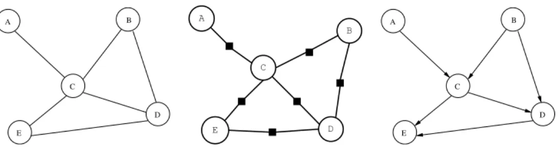
A C B D E A C B D E A C B D E

Figure 1: Three kinds of probabilistic graphical model: undirected graphs, factor graphs and directed graphs.

well, and we attempt to do Bayesian inference on them. To deal with intractability it is essential to have good tools for representing multivariate distributions, such as graphical models.

7 Graphical models

Graphical models are an important tool for representing the dependencies between random variables in a probabilistic model. They are important for two reasons. First, graphs are an intuitive way of visualising dependencies. We are used to graphical depictions of dependency, for example in circuit diagrams and in phylogenetic trees. Second, by exploiting the structure of the graph it is possible to devise efficient message passing algorithms for computing marginal and conditional probabilities in a complicated model. We discuss message passing algorithms for inference in Section 8.

The main statistical property represented explicitly by the graph is conditional independence between variables. We say thatX andY are conditionally independent given Z, ifP(X, Y|Z) =P(X|Z)P(Y|Z) for all values of the variables X,Y, and Z where these quantities are defined (i.e. excepting settings z where P(Z = z) = 0). We use the notation X⊥⊥Y|Z to denote the above conditional independence relation. Conditional independence generalises to sets of variables in the obvious way, and it is different frommarginal independencewhich states thatP(X, Y) =P(X)P(Y), and is denotedX⊥⊥Y.

There are several different graphical formalisms for depicting conditional independence relationships. We focus on three of the main ones: undirected, factor, and directed graphs.

7.1 Undirected graphs

In anundirected graphical model each random variable is represented by a node, and the edges of the graph indicate conditional independence relationships. Specifically, let X,Y, and Z be sets of random variables. ThenX ⊥⊥Y|Z if every path on the graph from a node inX to a node inY has to go through a node inZ. Thus a variableX is conditionally independent of all other variables given the neighbours ofX, and we say that the neighboursseparateX from the rest of the graph. An example of an undirected graph is shown in Figure 1. In this graphA⊥⊥B|C andB⊥⊥E|{C, D}, for example, and the neighbours ofD areB, C, E.

Acliqueis a fully connected subgraph of a graph. Amaximal cliqueis not contained in any other clique of the graph. It turns out that the set of conditional independence relations implied by the separation properties in the graph are satisfied by probability distributions which can be written as a normalised product of non-negative functions over the variables in the maximal cliques of the graph (this is known as the Hammersley-Clifford Theorem [10]). In the example in Figure 1, this implies that the probability distribution over (A, B, C, D, E) can be written as:

P(A, B, C, D, E) =c g1(A, C)g2(B, C, D)g3(C, D, E) (28)

Here, c is the constant that ensures that the probability distribution sums to 1, and g1, g2 and g3 are

non-negative functions of their arguments. For example, if all the variables are binary the function g2 is a

table with a non-negative number for each of the 8 = 2×2×2 possible settings of the variables B, C, D. These non-negative functions are supposed to represent how compatible these settings are with each other,

(14)

with a 0 encoding logical incompatibility. For this reason, theg’s are sometimes referred to ascompatibility functions, other times aspotential functions. Undirected graphical models are also sometimes referred to as

Markov networks.

7.2 Factor graphs

In a factor graphthere are two kinds of nodes, variable nodes and factor nodes, usually denoted as open circles and filled dots (Figure 1). Like an undirected model, the factor graph represents a factorisation of the joint probability distribution: each factor is a non-negative function of the variables connected to the corresponding factor node. Thus for the factor graph in Figure 1 we have:

P(A, B, C, D, E) =cg1(A, C)g2(B, C)g3(B, D), g4(C, D)g5(C, E)g6(D, E) (29)

Factor nodes are also sometimes called function nodes. Again, as in an undirected graphical model, the variables in a setX are conditionally independent of the variables in a set Y given Z if all paths from X

to Y go through variables in Z. Note that the factor graph is Figure 1 has exactly the same conditional independence relations as the undirected graph, even though the factors in the former are contained in the factors in the latter. Factor graphs are particularly elegant and simple when it comes to implementing message passing algorithms for inference (Section 8).

7.3 Directed graphs

In directed graphical models, also known as probabilistic directed acyclic graphs (DAGs), belief networks, and Bayesian networks, the nodes represent random variables and the directed edges represent statistical dependencies. If there exists an edge from A to B we say that A is a parent of B, and conversely B is a

childofA. A directed graph corresponds to the factorisation of the joint probability into a product of the conditional probabilities of each node given its parents. For the example in Figure 1 we write:

P(A, B, C, D, E) =P(A)P(B)P(C|A, B)P(D|B, C)P(E|C, D) (30) In general we would write:

P(X1, . . . , XN) = N

Y

i=1

P(Xi|Xpa_i) (31)

whereXpai denotes the variables that are parents ofXi in the graph.

Assessing the conditional independence relations in a directed graph is slightly less trivial than in undi-rected and factor graphs. Rather than simply looking at separation between sets of variables, one has to consider the directions of the edges. The graphical test for two sets of variables being conditionally inde-pendent given a third is called d-separation [64]. D-separation takes into account the following fact about

v-structures of the graph, which consist of two (or more) parents of a child, as in the A → C ← B sub-graph in Figure 1. In such a v-structure A⊥⊥B, but it is not true that A⊥⊥B|C. That is, A and B are marginally independent, but conditionally dependent given C. This can be easily checked by writing out P(A, B, C) =P(A)P(B)P(C|A, B). Summing out C leads to P(A, B) = P(A)P(B). However, given the value ofC,P(A, B|C) =P(A)P(B)P(C|A, B)/P(C) which does not factor into separate functions ofAand B. As a consequence of this property of v-structures, in a directed graph a variableX is independent of all other variables given the parents ofX, the children ofX, and the parents of the children ofX. This is the minimal set that d-separatesX from the rest of the graph and is known as the Markov boundary forX.

It is possible, though not always appropriate, to interpret a directed graphical model as a causal generative model of the data. The following procedure would generate data from the probability distribution defined by a directed graph: draw a random value from the marginal distribution of all variables which do not have any parents (e.g. a∼P(A), b∼P(B)), then sample from the conditional distribution of the children of these variables (e.g. c∼P(C|A=a, B=a)), and continue this procedure until all variables are assigned values. In the model,P(C|A, B) can capture the causal relationship between the causesAandBand the effectC. Such causal interpretations are much less natural for undirected and factor graphs, since even generating a sample from such models cannot easily be done in a hierarchical manner starting from “parents” to “children” except

(15)

Figure 2: No directed graph over 4 variables can represent the set of conditional independence relationships represented by this undirected graph.

in special cases. Moreover, the potential functions capture mutual compatibilities, rather than cause-effect relations.

A useful property of directed graphical models is that there is no global normalisation constant c. This global constant can be computationally intractable to compute in undirected and factor graphs. In directed graphs, each term is a conditional probability and is therefore already normalisedP

xP(Xi=x|Xpa_i) = 1.

7.4 Expressive power

Directed, undirected and factor graphs are complementary in their ability to express conditional independence relationships. Consider the directed graph consisting of a single v-structureA→C←B. This graph encodes A⊥⊥B but not A⊥⊥B|C. There exists no undirected graph or factor graph over these three variables which captures exactly these independencies. For example, inA−C−B it is not true thatA⊥⊥B but it is true that A⊥⊥B|C. Conversely, if we consider the undirected graph in Figure 2, we see that some independence relationships are better captured by undirected models (and factor graphs).

8 Exact inference in graphs

Probabilisticinferencein a graph usually refers to the problem of computing the conditional probability of some variableXi given the observed values of some other variablesXobs =xobs while marginalising out all

other variables. Starting from a joint distributionP(X1, . . . , XN), we can divide the set of all variables into

three exhaustive and mutually exclusive sets{X1, . . . XN}={Xi} ∪Xobs∪Xother. We wish to compute

P(Xi|Xobs=xobs) =

P

xP(Xi, Xother=x, Xobs=xobs)

P

x0 P

xP(Xi=x0, Xother=x, Xobs =xobs)

(32) The problem is that the sum over xis exponential in the number of variables in Xother. For example. if

there areM variables inXother and each is binary, then there are 2M possible values forx. If the variables

are continuous, then the desired conditional probability is the ratio of two high-dimensional integrals, which could be intractable to compute. Probabilistic inference is essentially a problem of computing large sums and integrals.

There are several algorithms for computing these sums and integrals which exploit the structure of the graph to get the solution efficiently for certain graph structures (namely trees and related graphs). For general graphs the problem is fundamentally hard [13].

(16)

8.1 Elimination

The simplest algorithm conceptually isvariable elimination. It is easiest to explain with an example. Con-sider computingP(A=a|D=d) in the directed graph in Figure 1. This can be written

What we did was (1) exploit the factorisation, (2) rearrange the sums, and (3) eliminate a variable,E. We could repeat this procedure and eliminate the variableC. When we do this we will need to compute a new functionφ(A=a, B=b, D=d)def= P

cP(C=c|A=a, B=b)P(D=d|C=c, B=b), resulting in:

P(A=a|D=d)∝X

b

P(A=a)P(B =b)φ(A=a, B=b, D=d)

Finally, we eliminateB by computingφ0(A=a, D=d)def= P

bP(B=b)φ(A=a, B=b, D=d) to get our

final answer which can be written

P(A=a|D=d)∝P(A=a)φ0(A=a, D=d) = P(A=a)φ

0₍_A₌_{a, D}₌_d₎

P

aP(A=a)φ0(A=a, D=d)

The functions we get when we eliminate variables can be thought of as messages sent by that variable to its neighbours. Eliminating transforms the graph by removing the eliminated node and drawing (undirected) edges between all the nodes in the Markov boundary of the eliminated node.

The same answer is obtained no matter what order we eliminate variables in; however, the computational complexity can depend dramatically on the ordering used.

8.2 Belief propagation

The belief propagation (BP) algorithm is a message passing algorithm for computing conditional probabilities of any variable given the values of some set of other variables in a singly-connecteddirected acyclic graph [64]. The algorithm itself follows from the rules of probability and the conditional independence properties of the graph. Whereas variable elimination focuses on finding the conditional probability of a single variable Xi givenXobs=xobs, belief propagation can compute at once all the conditionals p(Xi|Xobs=xobs) for all

inot observed.

We first need to define singly-connected directed graphs. A directed graph is singly connected if between every pair of nodes there is only one undirected path. Anundirected path is a path along the edges of the graph ignoring the direction of the edges: in other words the path can traverse edges both upstream and downstream. If there is more than one undirected path between any pair of nodes then the graph is said to bemultiply connected, or loopy(since it has loops).

Singly connected graphs have an important property which BP exploits. Let us call the set of observed variables the evidence, e = Xobs. Every node in the graph divides the evidence into upstream e+X and

downstreame−_X parts. For example, in Figure 3 the variablesU1. . . Untheir parents, ancestors, and children

(17)

X Y U U Y 1 1 n ... ... m

Figure 3: Belief propagation in a directed graph.

edge directed towardX are all considered to beupstreamofX; anything connected toX via an edge away from X is considered downstream of X (e.g. Y1, its children, the parents of its children, etc). Similarly,

every edgeX →Y in a singly connected graph divides the evidence into upstream and downstream parts. This separation of the evidence into upstream and downstream components does not generally occur in multiply-connected graphs.

Belief propagation uses three key ideas to compute the probability of some variable given the evidence p(X|e), which we can call the “belief” about X.4 _{First, the belief about} _X _{can be found by combining}

upstream and downstream evidence: P(X|e) = P(X, e) P(e) ∝P(X, e + X, e − X)∝P(X|e + X)P(e − X|X) (33)

The last proportionality results from the fact that given X the downstream and upstream evidence are conditionally independent: P(e−_X|X, e_X+) =P(e−_X|X). Second, the effect of the upstream and downstream evidence on X can be computed via a local message passing algorithm between the nodes in the graph. Third, the message from X to Y has to be constructed carefully so that node X doesn’t send back to Y any information thatY sent toX, otherwise the message passing algorithm would reverberate information between nodes amplifying and distorting the final beliefs.

Using these ideas and the basic rules of probability we can arrive at the following equations, where ch(X) and pa(X) are children and parents ofX, respectively:

Finally, the messages from parents to children (e.g.X toYj) and the messages from children to parents (e.g.

X toUi) can be computed as follows:

4_{There is considerably variety in the field regarding the naming of algorithms. Belief propagation is also known as the} sum-product algorithm, a name which some people prefer since beliefs seem subjective.

(18)

It is important to notice that in the computation of both the top-down message (36) and the bottom-up message (37) the recipient of the message is explicitly excluded. Pearl’s [64] mnemonic of calling these messagesλandπmessages is meant to reflect their role in computing “likelihood” and “prior” terms.

BP includes as special cases two important algorithms: Kalman smoothing for linear-Gaussian state-space models, and the forward–backward algorithm for hidden Markov models. Although BP is only valid on singly connected graphs there is a large body of research on its application to multiply connected graphs—the use of BP on such graphs is calledloopy belief propagationand has been analysed by several researchers [81, 82]. Interest in loopy belief propagation arose out of its impressive performance in decoding error correcting codes [21, 9, 50, 49]. Although the beliefs are not guaranteed to be correct on loopy graphs, interesting connections can be made to approximate inference procedures inspired by statistical physics known as the Bethe and Kikuchi free energies [84].

8.3 Factor graph propagation

In belief propagation, there is an asymmetry between the messages a child sends its parents and the messages a parent sends its children. Propagation in singly-connected factor graphs is conceptually much simpler and easier to implement. In a factor graph, the joint probability distribution is written as a product of factors. Consider a vector of variablesx= (x1, . . . , xn)

p(x) =p(x1, . . . , xn) = 1 Z Y j fj(xSj) (38)

whereZis the normalisation constant,Sj denotes the subset of{1, . . . , n}which participate in factorfj and

xSj ={xi:i∈Sj}.

Let n(x) denote the set of factor nodes that are neighbours of xand let n(f) denote the set of variable nodes that are neighbours of f. We can compute probabilities in a factor graph by propagating messages from variable nodes to factor nodes and vice-versa. The message from variablexto functionf is:

µx→f(x) =

Y

h∈n(x)\{f}

µh→x(x) (39)

while the message from functionf to variablexis:

µf→x(x) = X x\x  f(x) Y y∈n(f)\{x} µy→f(y)   (40)

Once a variable has received all messages from its neighbouring factor nodes we can compute the probability of that variable by multiplying all the messages and renormalising:

p(x)∝ Y

h∈n(x)

µh→x(x) (41)

Again, these equations can be derived by using Bayes rule and the conditional independence relations in a singly-connected factor graph. For multiply-connected factor graphs (where there is more than one path between at least one pair of variable nodes) one can apply a loopy version of factor graph propagation. Since the algorithms for directed graphs and factor graphs are essentially based on the same ideas, we also call the loopy version of factor graph propagation “loopy belief propagation”.

8.4 Junction tree algorithm

For multiply-connected graphs, the standard exact inference algorithms are based on the notion of ajunction tree [46]. The basic idea of the junction tree algorithm is to group variables so as to convert the multiply-connected graph into a singly-multiply-connected undirected graph (tree) over sets of variables, and do inference in this tree.

(19)

We will not explain the algorithm in detail here, but rather give an overview of the steps involved. Starting from a directed graph, undirected edges are introduced between every pair of variables that share a child. This step is called “moralisation” in a tongue-in-cheek reference to the fact that it involves marrying the unmarried parents of every node. All the remaining edges are then changed from directed to undirected. We now have an undirected graph which does not imply any additional conditional or marginal independence relations which were not present in the original directed graph (although the undirected graph may easily have many fewer conditional or marginal independence relations than the directed graph). The next step of the algorithm is “triangulation” which introduces an edge cutting across every cycle of length 4. For example, the cycleA−B−C−D−Awhich would look like Figure 2 would be triangulated either by adding an edgeA−C or an edge B−D. Once the graph has been triangulated, the maximal cliques of the graph are organised into a tree, where the nodes of the tree are cliques, by placing edges in the tree between some of the cliques with an overlap in variables (placing edges between all overlaps may not result in a tree). In general it may be possible to build several trees in this way, and triangulating the graph means than there exists a tree with the “running intersection property”. This property ensures that none of the variable is represented in disjoint parts of the tree, as this would cause the algorithm to come up with multiple possibly inconsistent beliefs about the variable. Finally, once the tree with the running intersection property is built (the junction tree) it is possible to introduce the evidence into the tree and apply what is essentially a variant of belief propagation to this junction tree. This BP algorithm is operating on sets of variables contained in the cliques of the junction tree, rather than on individual variables in the original graph. As such, the complexity of the algorithm scales exponentially with the size of the largest clique in the junction tree. For example, if moralisation and triangulation results in a clique containingKbinary variables, the junction tree algorithm would have to store and manipulate tables of size 2K_{. Moreover, finding the optimal triangulation}

to get the most efficient junction tree for a particular graph is NP-complete [4, 44].

8.5 Cutest conditioning

In certain graphs the simplest inference algorithm is cutset conditioning which is related to the idea of “reasoning by assumptions”. The basic idea is very straightforward: find some small set of variables such that if they were given (i.e. you knew their values) it would make the remainder of the graph singly connected. For example, in the undirected graph in Figure 1, given C or D, the rest of the graph is singly connected. This set of variables is called the cutset. For each possible value of the variables in the cutset, run BP on the remainder of the graph to obtain the beliefs on the node of interest. These beliefs can be averaged with appropriate weights to obtain the true belief on the variable of interest. To make this more concrete, assume you want to findP(X|e) and you discover a cutset consisting of a single variableC. Then

P(X|e) =X

c

P(X|C=c, e)P(C=c|e) (42)

where the beliefsP(X|C =c, e) and corresponding weights P(C =c|e) are computed as part of BP, run once for each value ofc.

9 Learning in graphical models

In Section 8 we described exact algorithms for inferring the value of variables in a graph with known parameters and structure. If the parameters and structure are unknown they can be learned from the data [31]. The learning problem can be divided into learning the graph parameters for a known structure, and learning the model structure (i.e. which edges should be present or absent).5

We focus here on directed graphs with discrete variables, although some of these issues become much more subtle for undirected and factor graphs [57]. The parameters of a directed graph with discrete variables parameterise the conditional probability tables P(Xi|Xpa_i). For each setting ofXpa_i this table contains a

5_{It should be noted that in Bayesian statistics there is no fundamental difference between parameters and variables, and} therefore the learning and inference problems are really the same. All unknown quantities are treated as random variables, and learning is just inference about parameters and structure. It is however often useful to distinguish between parameters, which we assume to be fairly constant over the data, and variables, which we can assume to vary over each data point.

(20)

probability distribution over Xi. For example, if all variables are binary and Xi has K parents, then this

conditional probability table has 2K+1 entries; however, since the probability over Xi has to sum to 1 for

each setting of its parents there are only 2K _{independent entries. The most general parameterisation would}

have a distinct parameter for each entry in this table, but this is often not a natural way to parameterise the dependency between variables. Alternatives (for binary data) are the noisy-or or sigmoid parameterisation of the dependencies [58]. Whatever the specific parameterisation, let θi denote the parameters relating

Xi to its parents, and let θ denote all the parameters in the model. Let m denote the model structure,

which corresponds to the set of edges in the graph. More generally the model structure can also contain the presence of additional hidden variables [16].

9.1 Learning graph parameters

We first consider the problem of learning graph parameters when the model structure is known and there are no missing or hidden variables. The presence of missing/hidden variables complicates the situation. 9.1.1 The complete data case.

Assume that the parameters controlling each family (a child and its parents) are distinct and that we observe N iid instances of all K variables in our graph. The data set is thereforeD={X(1). . . X(N)} and the likelihood can be written

P(D|θ) = N Y n=1 P(X(n)|θ) = N Y n=1 K Y i=1 P(X_i(n)|X_pa(n) i,θi) (43)

Clearly, maximising the log likelihood with respect to the parameters results in K decoupled optimisation problems, one for each family, since the log likelihood can be written as a sum of K independent terms. Similarly, if the prior factors over theθi, then the Bayesian posterior is also factored: P(θ|D) =QiP(θi|D).

9.1.2 The incomplete data case.

When there is missing/hidden data, the likelihood no longer factors over the variables. Divide the variables in X(n)into observed and missing components,X_obs(n)andX_mis(n). The observed data is nowD={X_obs(1). . . X_obs(N)}

and the likelihood is:

P(D|θ) = N Y n=1 P(X_obs(n)|θ) (44) = N Y n=1 X x(_misn)

P(X_mis(n)=x_mis(n), X_obs(n)|θ) (45)

= N Y n=1 X x(_misn) K Y i=1 P(X_i(n)|Xpa(n_i),θi) (46)

where in the last expression the missing variables are assumed to be set to the values x(_misn). Because of the missing data, the cost function can no longer be written as a sum ofKindependent terms and the parameters are all coupled. Similarly, even if the prior factors over theθi, the Bayesian posterior will couple all theθi.

One can still optimise the likelihood by making use of the EM algorithm (Section 3). The E step of EM infers the distribution over the hidden variables given the current setting of the parameters. This can be done with BP for singly connected graphs or with the junction tree algorithm for multiply-connected graphs. In the M step, the objective function being optimised conveniently factors in exactly the same way as in the complete data case (c.f. Equation (21)). Whereas for the complete data case, the optimal ML parameters can often be computed in closed form, in the incomplete data case an iterative algorithm such as EM is usually required.

Unsupervised Learning